Running CFD simulations on a single core allows us to perform simple 2D simulations, perhaps even with turbulence models activated, to extract some simple results. However, once we want to run some more realistic cases of industrial or academic relevance, we often have to utilise parallelisation to receive simulation results in a fraction of the time compared to a single-core simulation.
If parallelisation were a simple affair, i.e. simply telling our CFD solver how many cores to use and then expecting a proportional speed-up, we wouldn’t need this article, and CFD engineers would not be forced to work with eccentric computer scientists to get good parallelisation performance.
Parallelisation is a simple topic at first glance, but the devil is in the details. We will learn about how parallel performance is achieved on high-performance computing (HPC) clusters, which hardware is used, how to achieve good parallel performance (and how to quantify it), as well as the cost of parallelisation. We will also look at concrete code examples for parallelising a simple CFD solver using common parallelisation approaches for running simulations in parallel on the CPU and GPU.
If you have the feeling that parallelisation is a topic you haven’t spent much time with but ought to give it some attention, then this article is for you. It shows you how to extract the most computational power out of your simulations, how to use computational resources responsibly, as well as what bottlenecks exist in parallel computing that still require ongoing research.
It is one of those articles that likely takes a bit longer to read through, so I hope you have a strong brew next to you. This article was produced using approximately 31 TWINGINGS Earl Grey teas, 13 Meßmer Madame Grey teas, 17 17-grain Walnut-Almond teas, and about 5 KitKat hot chocolates. I recommend you consume the same. Here is to violent bladder failure.
Download Resources
All developed code and resources in this article are available for download. If you are encountering issues running any of the scripts, please refer to the instructions for running scripts downloaded from this website.
- Download: Parallelised Heat equation
In this series
- Part 1: How to Derive the Navier-Stokes Equations: From start to end
- Part 2: What are Hyperbolic, parabolic, and elliptic equations in CFD?
- Part 3: How to discretise the Navier-Stokes equations
- Part 4: Explicit vs. Implicit time integration and the CFL condition
- Part 5: Space and time integration schemes for CFD applications
- Part 6: How to implement boundary conditions in CFD
- Part 7: How to solve incompressible and compressible flows in CFD
- Part 8: The origin of turbulence and Direct Numerical Simulations (DNS)
- Part 9: The introduction to Large Eddy Simulations (LES) I wish I had
- Part 10: All you need to know about RANS turbulence modelling in one article
- Part 11: Advanced RANS and hybrid RANS/LES turbulence modelling in CFD
- Part 12: Mesh generation in CFD: All you need to know in one article
- Part 13: CFD on Steroids: High-performance computing and code parallelisation
In this article
- Introduction
- Flynn's taxonomy: The 4 types of parallelisation
- Understanding the hardware our simulations run on
- Performance and bottlenecks
- Parallelisation frameworks
- Challenges in code parallelisation for CFD applications
- Summary
Introduction
We all remember our humble beginnings in CFD. For me, it was the classical NACA 0012 simulation at a zero-degree angle of attack. While I rarely jump out of my seat these days when I see the contour plots around this airfoil, back then, I was blown away. It was so powerful that I decided that CFD is my calling, my passion, my future. I even went as far as changing my Facebook profile picture to this contour plot (is Facebook still alive?).
Chances are, your first simulation wasn’t much different, at least in terms of complexity. You likely ran a tutorial case that could be executed on your PC or laptop in a reasonable amount of time. Perhaps you made some changes to the input, played around with the test cases and, like me, realised that changes to the input had drastic effects on the simulation.
In my case, changing the angle of attack so that the airfoil would stall meant that convergence was no longer given. I found that fascinating and wanted to know more; others would have, understandably, given up, but then again, those would likely not commit to reading an unnecessarily long article on parallelisation and high-performance computing in CFD with the odd unhinged commentary.
Eventually, you and I gained confidence in our CFD skills, and we wanted to simulate our own cases, likely something more exciting than a 2D channel flow. So, we created 3D geometries and then realised that our PCs or laptops would not be able to run those simulations in a few minutes. I remember having my laptop and PC at that time running in parallel, both doing one simulation each and both running for about 24 hours per simulation. That was my first serious attempt at CFD; yours may have been similar.
But then, I was introduced to the world of high-performance computing (HPC). HPC to an aspiring CFD practitioner is like the discovery of Viagra for a retired Person; it’s a game changer (or starter?). All of a sudden, I was able to run simulations in less than an hour that would otherwise take me days. This was reason enough to get acquainted with HPC, even though there was a step learning curve (I also had an HPC assignment due, which likely contributed to my motivation).
When we are dealing with HPC, we typically mean HPC clusters, which sometimes are also called supercomputers, because whoever came up with this name was suffering a lack of serious creativity. Here are my takes:
- The Mother of all FLOPs (MOAF)
- Clusterfuck
- Cache Me If You Can
An HPC cluster is nothing but a bunch of PCs chained together. The simplest cluster we can think of is a bunch of Raspberry Pies linked together. There is even an official tutorial by the makers of Raspberry Pi, showing you how you can do that. It is weirdly affordable, and you can decide next time you buy a new gaming PC if you really need that or your own HPC cluster on your desk.
While the Raspberry Pi example is good to understand how a cluster works, if we need serious computing power, as we do for CFD applications, we really want to use dedicated hardware. All major chip manufacturers offer dedicated compute hardware to build clusters, and these are somewhat different to what you would find in PCs and laptops. The main difference is speed and performance. They have more cores, more memory, and a network connection so fast that it would melt your router (maybe).
Twice a year, TOP500 uploads a list of the 500 fastest clusterfucks HPC clusters in the world. They list, among other details, the number of cores, the performance, as well as the power required to keep the cluster running. The performance is measured in how many floating-point operations can be done per second on the cluster. The unit is PFLOPs, or Peta Floating-point Operations Per second, where Peta stands for 10^{15}.
If we designed a new cluster, and we could get a staggering 1 PFLOPs in performance, we could perform 10^{15} multiplications/divisions/additions/subtractions per second on floating point numbers. Let’s put this into perspective. If we have a mesh with 10 billion cells, we have 10^{10} cells. We can perform 10^{15} / 10^{10} = 10^5, or 100,000 operations per second on each cell. Imagine what you could simulate with 10 billion cells. Direct Numerical Simulations (DNS) would be the norm.
Where would this impressive cluster rank in the TOP500? Nowhere. 1 PFLOPs in performance isn’t impressive any more, and we likely wouldn’t even make the top 1000. These days, we have achieved exascale computing. That is, instead of measuring performance in PFLOPs, we use EFLOPs, or Exa FLOPs. Exa stands for 10^{18}, and the best supercomputers in the world go beyond 1 EFLOPs.
All of this performance needs to be leveraged, and this is where code parallelisation comes in. We can’t just write a CFD solver and then hope that our HPC cluster will be able to run it. If we write software without consideration given to parallelisation, we can’t use more than one core. There is no point running our software on a 10-million-core cluster if we can only use one of them.
Thus, we need to parallelise our code, meaning we have to modify our code so it can use more than 1 core. With that come unique challenges, and I want to explore those in this article, as well as performance metrics that help us to measure if we have achieved a good parallel performance, and some frameworks we can use to parallelise our code.
We have our work cut out for ourselves; let us see how we can do that.
Flynn’s taxonomy: The 4 types of parallelisation
Flynn’s taxonomy allows us to identify 4 separate parallelisation approaches based on instruction and data parallelism. If we are dealing with multiple instructions, each processor will work on separate instructions. If we have multiple data sets, this means that processors work on different data. An overview of Flynn’s taxonomy is given in the following figure:
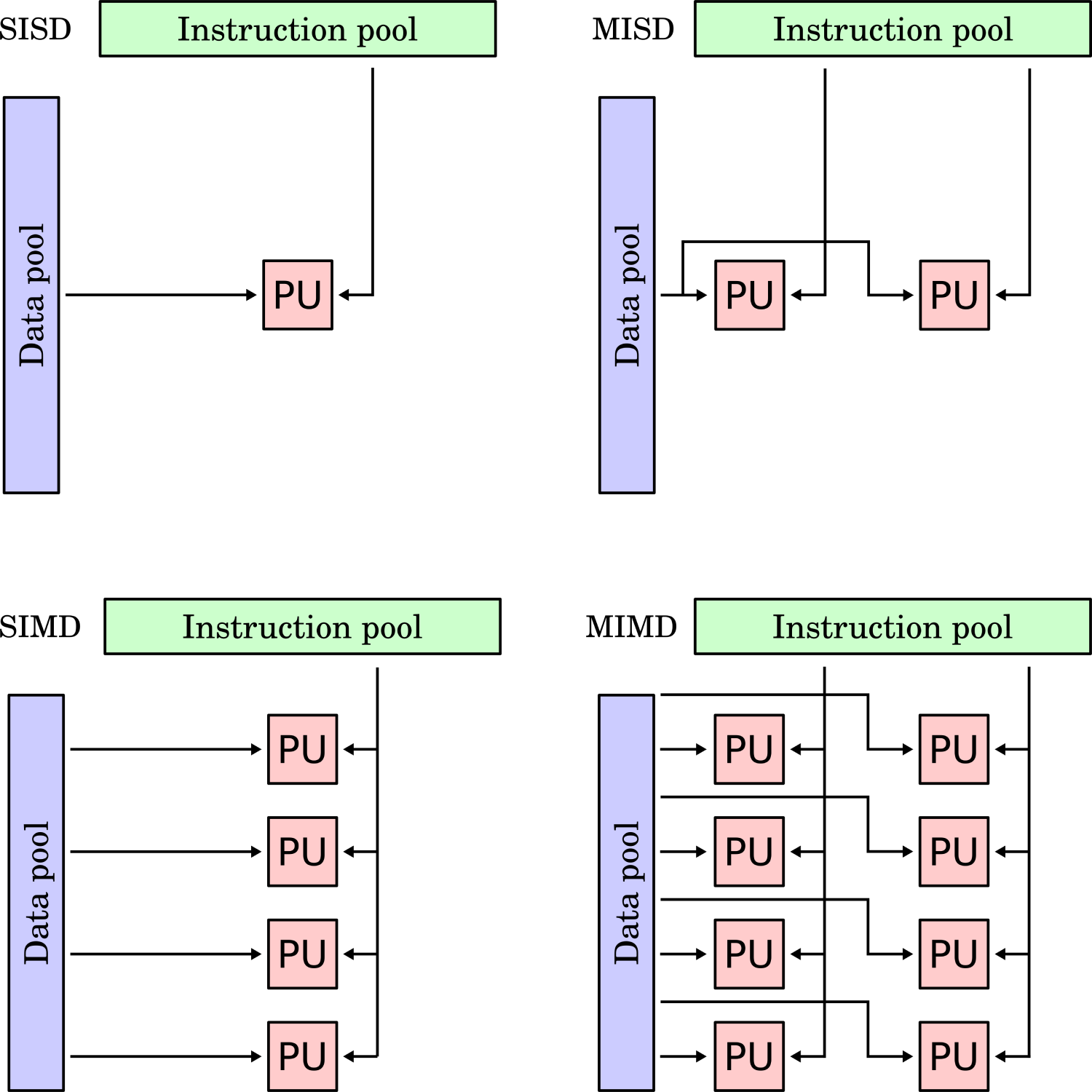
When I first saw this classification, I had difficulties understanding it; it seemed a bit abstract. So let’s breathe some life into this figure and give examples for each quadrant.
Single instruction, single data (SISD)
Single instruction, single data (SISD) is the paradigm you will be most familiar with. It means we have a single instruction, executed by a single processor, and it is working on a piece of data. If you have ever written a simple CFD solver, even just a code to solve a model equation like the heat diffusion, advection, or Burgers equation, you wrote a SISD program.
You had a single core working through your instructions, e.g. first compute the gradients, then perform the time integration, then update the solution, etc. All of this was performed by a single processor, and all of this was done one at a time. In terms of data, that was coming from RAM, and all of that RAM was available to you. Thus, your processor used only one set of instructions, and it was operating in a single set of memory. This is also called a sequential application.
Single instruction, multiple data (SIMD)
Single instruction, multiple data (SIMD) is the most important parallelisation category for us in CFD. When we talk about code parallelisation, we talk about SIMD parallelisation. Code parallelisation means that we now use more than one processor to run our code. All processors execute the same instruction, but they operate on different data.
In practice, this means that each processor will still perform the same steps as in our previous example, i.e. each processor will compute gradients, then integrate in time, etc. They will all work at the same time but on different data. This means that if I want to parallelise my code and I run a simulation with a 10 million cell mesh on 4 processors, each processor will perform the gradient calculation, time integration, etc., on only 2.5 million cells.
The speed-up, then, is coming from the fact that for each individual processor, it seems like the problem size is only 2.5 million cells, rather than the full 10 million cells, and so in an ideal world, we would expect (or rather, hope) that we can a 4-times faster simulation with 4 processors compared to a single processor simulation (e.g. SISD).
Multiple instruction, single data (MISD)
Multiple instruction, single data (MISD) is a concept that only really exists for completeness in Flynn’s taxonomy. While this parallelisation does exist in the real world, it does not make sense in the world of high-performance computing. The reason is that MISD performs multiple different instructions, but all on the same data. If we take the example from before, each processor gets the full 10 million cells mesh. If they all have to operate on it, we won’t see a speed-up.
So why would we ever use this? In systems where redundancies are important, MISD is the way to go. For example, an aeroplane measures airspeed with 3 different sensors. It does that because knowing the airspeed is the difference between flying and stalling (and thus falling out of the sky). Thus, the onboard computers that calculate the airspeed are getting their input from three separate sensors (which all provide the same data), and because we have more than one computer, we have multiple instructions operating on this single dataset.
So, MISD is an important paradigm, but just not in high-performance computing.
Multiple instruction, multiple data (MIMD)
If you like complexity, then Multiple Instruction, multiple data (MIMD) is for you. It contains the same multiple data concept we already saw in SIMD, and this really is where computational gains are coming in (breaking a larger problem down into smaller subdomains and solving these smaller subdomains for faster simulation times).
With MIMD, we open ourselves up to multiphysics problems. The simplest and most studied one would be Fluid-Structure Interactions (FSI). Here, we solve a CFD problem and couple that with an FEA solver. Both the CFD and FEA solver have their own data to work on (multiple data). A CFD solver also would have different instructions compared to a FEA solver (multiple instructions), e.g. there is no “solve continuity equation” in the FEA solver, nor is there a “compute displacements and von Mises stresses” in the CFD solver.
Whenever we are coupling two or more solvers together, we get into multiple instructions territory. As long as we leverage multiple data as well, we have a viable parallelisation strategy. The challenges arise here in determining which resources to allocate to which solvers. If we want to perform a single time integration between CFD and FEA, then the FEA solver may only take 1/5 of the time to update the timestep compared to the CFD solver. If we give them the same resources, the FEA solver will waste most of them.
Thus, we need to think about how to balance resources allocated to each solver, and this is known as load balancing. This is a crucial aspect in high-performance computing, and if we don’t have a good load balance in our simulation, all of our code parallelisation is pointless.
For completeness, load balancing also affects SIMD, i.e. if we have 10 million cells and 4 processors, we want to make sure that each processor gets an equal amount of work (i.e. 2.5 million cells). If we give 3 processors just 1 million cells and the remaining processor 7 million cells, then we are going to have a load imbalance. On paper, this may seem like a simple problem, but in reality, it isn’t, and we will talk a lot more about the challenges later when we deal with domain decomposition techniques.
Understanding the hardware our simulations run on
Understanding computer hardware is really important if you want to understand how performance is achieved (or lost). You may think, for example, that once your code is parallelised, you get an automatic speed-up if you use more processors. This is certainly the approach I see new students make. Whenever I ask them why they are using 96 processors for their simulation, the answer is usually “because that is the maximum I am allowed to use“. That is the wrong answer.
If you have access to a CFD solver, set up a simple test case, something with 10000 cells or less and then run this on 1 processor and the max number of processors available to you. Say you have a 4-core CPU, then run this with 4 processors. What you will see is that your 4-processor simulation is slower than your 1-processor simulation.
The opposite can also happen. Say you set up a simulation to run on a single core. You then parallelise your code and run the simulation on 4 processors. You would expect the simulation to speed up by, at most, a factor of 4. You measure the speed up, and you see that your actual speed up is 5. All of this can be explained by understanding the computer hardware.
Some time ago, my beloved custom-built CFD workstation PC died (I say custom-built CFD workstation, this is the excuse we give ourselves to splurge on a high-spec PC to run some CFD simulations, only to realise that your CFD workstation is also an excellent gaming rig. The amount of yoghurt and excavators I have delivered to Scotland in European Truck Simulator 2 is embarrassingly high … just me?).
I must have told that story before, but in a nutshell, driving at night gives probably the best immersion, but trucks also have quite a few gears, and so I was busy shifting gears while traversing the Scottish Highlands. It turns out that if your partner tries to sleep in the same room, those gear shifts are really annoying, and she told me as much. Suffice it to say, I no longer have access rights to my steering wheel.
In any case, that PC died, and so I bought another somewhat decent PC, at least spec-wise. It had a GIGABYTE motherboard, a brand I had no idea existed before, but it seemed legit, so I didn’t question it. The PC arrived, worked a good 2 months, so the PC could no longer be returned, and at that point, the PC started to crash hard. 10 bluescreens of death or more were common per day, and they would happen out of the blue (no pun intended).
After trying to reinstall Windows about 10 times, changing hardware, and examining crash dumps, I was ready to give up on my PC. And then, I saw this video:
Apparently, the motherboard I had came with malware on the hardware level. No matter what changes I made to my operating system, the motherboard would randomly crash my PC, and that’s also why all of the crash dumps would not make any sense whatsoever. I upgraded the BIOS, but even that wasn’t working. So, the issue may have been somewhere else entirely, but I could not be bothered investigating this further.
I told my line manager that my PC died and I needed a new CFD workstation. I got another beefy machine, and while I use it for work (I am writing this article currently on it), it is also exceptionally well-suited to play Rocket League on it. Who would have thought?
There is a point to make here (believe it or not). I thought I could tell you about this PC story and then transition to the PC hardware. I wanted to take a picture of that PC (for some reason, I still hold on to it) and show you the motherboard, RAM, CPU, GPU, hard disk, etc. and then go through each component and say something like “this is the most expensive picture I ever took”, as in, I can’t use it anymore as a PC, so it is essentially an expensive photo model. But then I took the picture, and this is what I got:
Wow, I can show you where the fan is sitting, and that’s probably it. Why is there so much empty space (and dust)? It is not just a bad PC, it’s also a pretty bad photo model. Turns out I should have just googled a motherboard picture and saved you from my random sidebar, but you are still here, so you get partial blame, too.
So, let’s look at a normal motherboard:
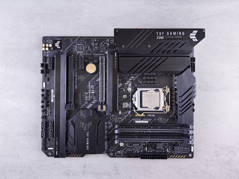
Most will likely be familiar with this. We have our central processing unit (CPU) in the middle, slightly to the right (hidden under the metallic cover). Below that are 4 slots to insert random access memory (RAM) modules, and to the left are 2 Peripheral Component Interconnect (PCI) slots for graphical processing units (GPUs). Well, there are other things we could put here, but typically, we only place GPUs here.
I like this motherboard because on the top right, it states: “TUF GAMING Z590 MILITARY GRADE PERFORMANCE”. What exactly is military-grade performance? I know that products sometimes boast military-grade durability when they follow, for example, the military standard for stress testing. But what is military-grade performance? As one source succinctly puts it: Military-grade is just military-grade marketing bullshit. Moving on.
We can summarise that a normal PC, or laptop, will have a CPU, some RAM, some main memory (hard disk), as well as potentially some add-on devices like a GPU. Add some cooling for CPUs and GPUs to avoid overheating, and you have yourself a PC. Probably, I am not telling you anything new here. But let’s now explore what a high-performance computing cluster looks like.
The following schematic shows how an HPC cluster is structured.
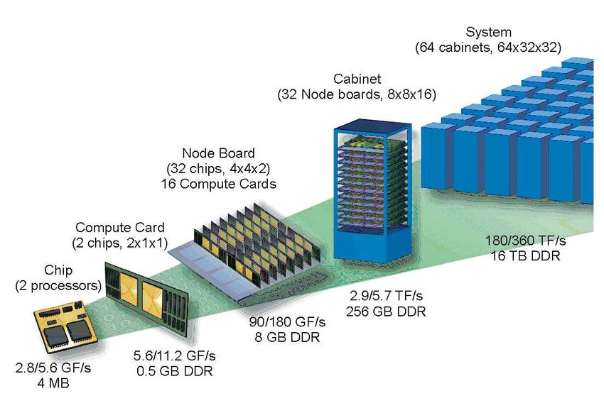
Starting on the right, we have the entire HPC cluster. Its size is usually large enough to warrant building an entire building around it, which is sometimes misleadingly called a data centre (though data centres can also be interpreted as a catch-all name for anything from long-term storage (e.g. Dropbox), to cloud computing, to high-performance computing clusters).
The HPC cluster, or system, is made up of individual cabinets. Each of these cabinets will house a number of racks (which are called node boards in the schematic above), which contain a number of compute nodes (called compute cards in the schematic above). If you are talking to a professional, they may just use the word node, and it appears that the infantile urge to abbreviate everything (LOL, ROFL, LMAO, yes, I know, I’m old) does not stop when you have a PhD (which is an abbreviation as well, now that I think about it …).
Each node (oh no, I am one of them), I mean, each compute node, may contain one or more sockets. There are different names for the same thing, but a socket is equivalent to a CPU on a consumer PC or laptop. Essentially, each socket will contain a number of so-called cores, or processors. On a consumer PC, we may have a 4-core CPU, but in HPC land, we typically have quite a few more per socket, starting at 16 cores, and going up to 64 or even 128 cores.
Let’s look at some real examples. The figure below shows a typical HPC cluster, as you may find it in the wild.

Again, whoever is setting up HPC clusters seems to spend a lot of effort on making HPC clusters look sexy. Some will plaster wallpapers all over the place, some will install mood lighting, and how is this different from a script kiddie spending way too much on LED lights for their gaming PC?
The more I think about it, people working in HPC are just grown-up kids. And after this thought entered my mind, I just couldn’t stop thinking that everyone in the Harribo commercials is just someone working as an HPC admin. I mean, how is the following not an annual meet-up of HPC admins?
Congratulations, you just watched an advert, and no, of course I’m not getting paid for this (did you really think Harribo is sponsoring me?). Moving on.
Within each cabinet, we have our racks, each stuffed with compute nodes, and this is shown below:
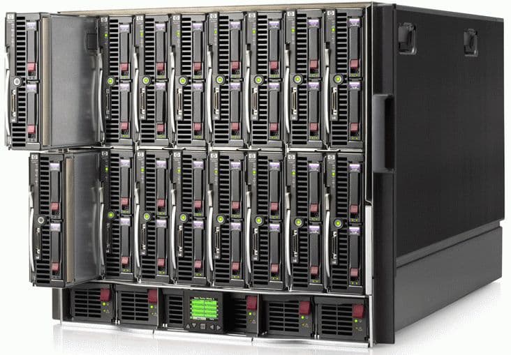
If you click through to CTO servers, you’ll see that this beauty is sold as a stand-alone OpenFOAM HPC cluster. And I may add, looking at the specs, it is very reasonably priced … I might get one for myself … (I’m not, (and, no, again, not getting paid to promote them either, just think this is a cool product, but I love bare metal hardware, you can sell me anything)).
If we take one of the compute nodes out of the rack, we start to see hardware that finally resembles a consumer PC or laptop. This is shown below:
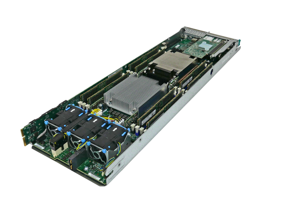
Here, we have two sockets in the centre, both shielded by a metallic heat exchanger device. Each socket may contain 16, 32, 64, or 128 cores, typically, and so if we have two of these sockets per node, we may end up with a total of 32, 64, 128, or 256 cores per node. That is some serious computing power! To either side of the sockets, we have our main memory (RAM), and we have some fans at the bottom.
Other compute nodes may additionally house a small GPU as an add-on, though we can also get entire GPU nodes. If you want to have some fun, google “what is the most expensive Nvidia GPU”. At the time of writing, the H100 is still leading the market with its ~£30,000 price tag. For the same money, you can almost get a Tesla Model S, and I am sure we are not far away from Nvidia’s GPU becoming more expensive than electric cars.
I mean, at this rate, we may see celebrities start to wear Nvidia GPUs as status symbols instead of jewellery or fashion brands. Me: “Create a picture of a celebrity of your choice wearing a Nvidia GPU like a status symbol”. ChatGPT:

There are three possibilities for how we can create our HPC system. Either we have a homogeneous system, using only CPUs or GPUs, or we have a heterogeneous system, having a mix of CPUs and GPUs. Most HPC systems these days are heterogeneous and cater for both CPU and GPU applications, though you will find more and more dedicated GPU clusters, which are predominantly used for AI, so we can create a pointless cartoon impression of celebrities wearing GPUs as status symbols.
Another important aspect of HPC clusters is their network. Nodes and cabinets are typically connected through a very high-throughput and low-latency network. A common choice here is the InfiniBand standard. As we will see, in most of the cases we are interested in (SIMD CFD applications), our bottleneck is memory transfer, and we spend a lot of effort squeezing the last bit of performance out of our code by placing the data as close as possible next to each other to reduce memory transfer time.
There are different mechanisms by which we can achieve that, and we will look at them later in this article. But for now, I think we have gotten a good overview of the HPC hardware and architecture. Let us now explore how we can measure performance in our codes, some bottlenecks for our performance, as well as some considerations that are less commonly discussed in the HPC literature.
Performance and bottlenecks
OK, so we have access to a few cores now, either through our CPU on our laptop/PC, heck, even our smartphones these days come with an 8-core CPU (this will age like milk …), we want to leverage them. We may even have access to a decent cluster, and we may be able to use a few hundred cores, for example. Should we always use all of the computational resources we have available?
For each simulation we run, there is an optimal number of cores, and so we want to know at which level of parallelism (i.e. how many cores) we get the most performance (reduction in computational time). Beyond that point, we will start to increase the computational cost (i.e. we use more cores, requiring more energy), and the performance will decrease (increase in computational time).
Thus, we want to find out what the optimum number of cores is. There is no one-size-fits-all answer, and the optimum number of cores is a code-specific number. But there are ways in which we can establish that numerically, and so in this section, we will look at this in more detail.
The optimum number of cores is not the only thing we want to look at, though, even though the answer may be that we should be running our simulation on 128 cores for 2 days, we should ask ourselves if we really need to. Do we need to run this simulation? This question seems odd, and is probably never asked, but once we look into the economics of running large-scale simulations, we realise that we are quite heavily polluting the atmosphere with CO_2.
So the question: “Are we getting enough information out of this simulation to justify the electricity usage and CO_2 release” becomes a relevant and highly important question.
For example, if we want to run a Large Eddy Simulation (LES) around an airfoil at various angle of attacks, just to get a better prediction of the critical (stall) angle of attack, compared to a much cheaper Reynolds-averaged Navier-Stokes (RANS) simulation, we should calculate the expected electricity usage and CO_2 release for both cases and make a judgement on whether we can justify the cost for obtaining a single value with a somewhat improved predictive quality.
We may come to the conclusion that no, it is not justified, and that perhaps other approaches can be explored. For example, we can create a 2D RANS mesh with a lot more resolution than our 3D LES grid and get a transitional RANS model to predict the stall angle with perhaps a slightly less accurate prediction, but with a significantly reduced computational cost.
These trade-off considerations are not commonly done. CFD practitioners are not seeing the energy bill, nor do they see any environmental reports on how their HPC usage contributes to their CO_2 footprint.
I bring this up because I generally observe a lack of awareness in my students when they run a simulation. They get upset when they can’t run as many simulations as they want for their MSc thesis, but then run simulations on the cluster that fail after some time because they were not thoroughly tested. Sometimes these simulations don’t even add value, and so my original question, “Are we getting enough information out of this simulation to justify the electricity usage and CO_2 release” is not that strange after all and highly relevant!
Let’s now discuss a few metrics we can use to assess the parallel performance, and then circle back to the environmental considerations afterwards.
Amdahl’s law
Amdahl’s law is a simple yet very educational law we can use to assess parallel performance. It is so simple that it is easy to understand, yet it gives us some surprising results, especially if we have never seen it before.
Let’s think about parallelism for a moment. Our goal is to use more than one core in the hope that our simulation time will reduce proportionally to the number of cores that we are using. As a simple example, we may say that a simulation may run exactly for 32 minutes using a single core. Then, if I use 2 cores, I would hope that my simulation only takes 16 minutes. If I use 32 cores, I would hope that my simulation only takes 1 minute. That is parallelisation in a nutshell.
But there are things which cannot be parallelised. For example, if I run on 32 cores and I want to print something to the console, like my residuals, or some information about the current time step, like the timestep size and total elapsed simulation time, only one processor will do that. If all 32 processors did that, we would get the same information printed 32 times.
Writing data to the hard drive is another aspect that is difficult to parallelise, although there are non-trivial options to do this with MPI I/O and HDF5, for example, it is a task that may also be done by only one processor. So, there will always be some portion of the code that cannot be parallelised, and we will never get a code with 100% parallelism.
How could we express that mathematically? Let’s say that T is the total time it takes to run our simulation, so 32 minutes on 1 core, 16 minutes on 2 cores, and so on. Then, we can introduce two additional times. T_{par} is the execution time of the code that can be parallelised, while T_{no-par} is the part of the code that cannot be parallelised (writing to the console, or hard drive, for example). Thus, the total time is:
T=T_{no-par} + T_{par}
\tag{1}
So far so good (and simple). Now, let us try to express T_{no-par} and T_{par} as functions of T alone. For that, we will introduce a fraction f that is in the range of [0,1]. A value of f=0.8, for example, would say that 80% of our code can be parallelised. The way we could determine that, for example, is to go through each line of our code and see if it is executed in parallel or not. Then we may have 80 lines of code that run in parallel out of 100 lines of code, so f=80/100=0.8.
We can now start to weight the contributions in Eq.(1) with:
T_{no-par} = (1-f)T\\
T_{par} = fT \\
T = (1-f)T + fT
\tag{2}
So, we have now found a way to express the total computational time as a weighted sum of the parts of the code that can be parallelised and that cannot. Let’s now also consider the speed-up s. This is the factor by which we reduce our computational time after parallelising our code. Let’s make the example simple. Let’s say f=1, so everything can be parallelised. Then, we have:
T=fT\tag{3}If we wanted to compute the speed-up, we would have to divide the right-hand side by s, i.e. we get:
T=\frac{f}{s}T\tag{4}Now, we can say f=1, so if we use 32 cores for our 32-minute simulation, we get:
1\, min=\frac{1}{32}32\, min\tag{5}But now let’s extend that for cases where f isn’t 100%. So we bring back our weighted sum from Eq.(2). This results in:
T = (1-f)T + \frac{f}{s}T
\tag{6}
We do not divide (1-f)T by s because that is, by definition, the part of the code that cannot be parallelised, and so we cannot speed up this part of the code. Therefore, only the part that can be parallelised will benefit from the speed-up.
Eq.(6) will give us the time it takes to run our simulation on p processors. We can denote this time by T(p,f), where we also include the fraction of the code that can be parallelised, i.e. f. Thus, Eq.(6) becomes:
T(p,f) = (1-f)T + \frac{f}{s}T
\tag{7}
Remember that T is the total time it takes to run the simulation. On a single processor, this would be T(1,f) = T by definition, because there is nothing to parallelise on a single core (we could also say that f=0). This would give us the same result, i.e.:
T(1,f) = (1-0)T + \frac{0}{s}T = T\tag{8}If we wanted to know the speed-up as a function of the fraction of the code that can be parallelised, i.e. f, we compute the ratio of T(1,f)/T(p,f). This results in:
\frac{T(1,f)}{T(p,f)} = \frac{T}{(1-f)T + \frac{f}{s}T}
\tag{9}
We can simplify this equation as:
\frac{T(1,f)}{T(p,f)} = \frac{T}{(1-f)T} + \frac{T}{\frac{f}{s}T} = \frac{1}{1-f}\frac{T}{T} + \frac{1}{\frac{f}{s}}\frac{T}{T} = \frac{1}{1-f} + \frac{1}{\frac{f}{s}} = \frac{1}{(1-f) + \frac{f}{s}}
\tag{10}
This is an important finding, so let me write the final result again so it stands out better:
\frac{T(1,f)}{T(p,f)} = \frac{1}{(1-f) + \frac{f}{s}}
\tag{11}
This is Amdahl’s law, and it tells us that we can compute the theoretical speed-up knowing only the portion of our code that can be parallelised f and the speed-up s. We can use this to determine upper bounds for our parallelisation efforts. This is shown in the next figure:
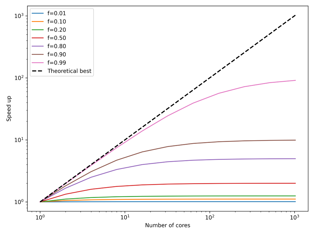
What I have done here is to plot the speed up, on the y-axis, we can expect for any number of cores, given on the x-axis. I have also plotted the theoretical best parallelisation, that is, if all of our code can be run in parallel. This is shown as the theoretical best line, and this corresponds to f=1. I have plotted how our speed-up converges to a fixed value, regardless of how many processors we are using (we are assuming here that the speed-up s is proportional to the number of cores).
Thus, we can see that there are diminishing returns if we use more and more processors, and we can even compute the upper bound with Amdahl’s law, what the best performance s_{opt} is that we can expect. To do that, we have to compute:
s_{opt} = \lim_{s\rightarrow \infty}\frac{1}{(1-f) + \frac{f}{s}} = \frac{1}{1-f}\tag{12}Thus, the best speed up is determined not by the part of the code that can be parallelised, but rather by the part that cannot be parallelised, which is 1/(1-f). So, we can find s_{opt} numerically for different values of f as:
- f=0.01 \rightarrow s_{opt} = 1.01
- f=0.10 \rightarrow s_{opt} = 1.11
- f=0.20 \rightarrow s_{opt} = 1.25
- f=0.50 \rightarrow s_{opt} = 2.00
- f=0.80 \rightarrow s_{opt} = 5.00
- f=0.90 \rightarrow s_{opt} = 10.00
- f=0.99 \rightarrow s_{opt} = 100.00
This means that the number of cores we have available is not really important. Much more important is how well our code has been parallelised. Even if 99% of our code can execute in parallel, we can expect, at best, a speedup of 100. So, if we have access to, say, 1000 cores, we wouldn’t be able to use all of them. We would be limited by the theoretical speed-up of 100, at most. In order to use all 1000 cores, we would first have to ensure that we have at least 99.9% of our code parallelised.
These numbers may seem frightening, but in reality, it isn’t that difficult to achieve parallelisation of 99.9% or even more. Look at scientific articles where people run their simulations with 10,000 cores or more successfully, i.e. seeing a corresponding speed-up. It is possible.
Having said that, I should also state that we like to cheat a bit in CFD (everybody is doing it, so that makes it Ok, right?). We typically ignore large portions of our code, and only measure the part of the code that has been parallelised. Things like reading a mesh, allocating memory, etc., are not considered. We only look at our time or iteration loop, which can, in general, be easily parallelised. This is where most of the computational time is spent, which justifies this approach.
The takeaway message is that Amdahl’s law tells us that we cannot just throw an infinite number of processors at our problem; eventually, we will reach a ceiling beyond which we cannot expect more performance.
Amdahl’s law is a good theoretical model to sensibilise ourselves to the fact that there are diminishing returns as we increase the number of cores. However, in reality, it is very difficult to know what the fraction f is of our code (it turns out, just counting the lines of code isn’t a reliable indicator, and even worse, if we have 1 million lines of code or more, who’s got the time to do that?).
So, we need a different metric that embodies the same information as Amdahl’s law, but we can access that information by just measuring the performance of our code. This is where weak and strong scaling come in, and these are discussed in the next sections.
Strong scaling
The strong scaling measures the speed-up of a parallel code execution. We keep the problem size the same and only change the number of cores. We want to measure how the speed-up changes as we increase the number of cores. We can define the speed-up as:
s(p) = \frac{T(1,N)}{T(p,N)}
\tag{13}
We use a slightly different notation here compared to the previous section. Here, p is the number of cores we are using, just as before, but N is now the problem size. In our case, it would typically be the number of cells in our mesh. If we are dealing with a finite element discretisation, N would be the number of degrees of freedom (since we can have more than a single integration point per cell). Regardless of which approach we chose, N is always proportional to some characteristic size we can state about our problem.
The time it takes to run the simulation on one core is given as T(1,N). The time it takes to run the simulation on p cores is T(p,N), and the ratio of the two gives us the speed-up, as seen in Eq.(13). Let’s look at some sample numbers, which were taken from HPC-wiki. The table below shows typical numbers you may find when you measure the execution time of your code as you increase the number of cores.
| Number of cores (required nodes) | Measured time (in seconds) |
|---|---|
| 1 (1 node) | 64.4 |
| 2 (1 node) | 33.9 |
| 4 (1 node) | 17.4 |
| 8 (1 node) | 8.7 |
| 16 (1 node) | 4.8 |
| 32 (1 node) | 2.7 |
| 64 (2 nodes) | 1.6 |
| 128 (4 nodes) | 1.0 |
| 256 (8 nodes) | 1.4 |
| 512 (16 nodes) | 3.7 |
| 1024 (32 nodes) | 4.7 |
| 2048 (64 nodes) | 21.5 |
In the left column, we see the number of cores required, as well as how many (compute) nodes we need. In this case, each compute node has 32 cores. On the right, we show the measured time it took to run a given simulation on the given number of cores.
We need to be careful how we obtain these time measurements. We can’t just go to our cluster, run a simulation for a number of cores, record the time, and then move on. If we do that, we will get a lot of noise, or variance, in our results. Instead, we should run the same simulation over and over again. With a number of measurements available, we can now either compute the average time or take the shortest time. I have seen both approaches being used in the wild.
When CPUs are not in use, they are typically underclocked to save energy. So, if you throw your simulation onto a compute node that was idling for some time before you showed up with your (simulation) problems, it is likely that the process of bringing the compute node back up to speed will influence your measured compute time. In this case, we may want to give the compute node a task to do for a few seconds before we start measuring simulation times.
If we compute the speed-up now based on the time measurements we saw above in the table, then we can plot it against the number of cores. This is shown in the figure below on the left:
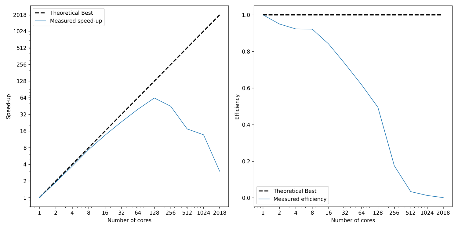
I have shown here two lines; the first (dashed) line shows the best possible speed-up. That is, if we use p processors, then a speed-up of p is the best possible scenario we can expect. While we see that the measured speed-up, shown as a solid blue curve, follows this trend initially, it starts deviating from it relatively soon. At around 128 cores, we see a peak. Afterwards, the speed-up is going down again.
This is the expected behaviour. In order to understand that, we need to know more about how code parallelisation works (and we will look at that in more detail). But in a nutshell, imagine we want to compute the gradient of the velocity field in the continuity equation. Thus, we may have a finite difference approximation as:
\nabla\cdot\mathbf{u}=\frac{\partial u}{\partial x} + \frac{\partial v}{\partial y} + \frac{\partial w}{\partial z} = 0\\[1em]
\nabla\mathbf{u}\approx \frac{u_{i+1, j,k} - u_{i-1,j,k}}{2\Delta x} + \frac{v_{i, j+1,k} - v_{i,j-1,k}}{2\Delta y} + \frac{w_{i, j,k+1} - u_{i,j,k-1}}{2\Delta z} = 0\tag{14}
Let’s look at u_{i+1, j,k} and u_{i-1, j,k}. We said before that in order to achieve faster code execution, we may split a 10-million-cell problem over 4 processors, where each processor is now solving only a 2.5-million-cell problem. This means that our original mesh is now chopped up into smaller chunks. But, if we compute the solution near or at the boundary of one of these subdomains, then we may find that u_{i+1, j,k} is still on our domain, but u_{i-1, j,k} isn’t.
It turns out that u_{i-1, j,k} is on the neighbouring subdomain, and so we have to request now a copy of that from our neighbour. So, we send a request, and we wait. Imagine you need a vital piece of information, but you don’t have it. But, you know who has it. So, you may send that person an email and wait for their response. Once they get back to you, you can continue to work, but in the meantime, you are waiting for a response before you can continue.
The same is true for our request to get data for u_{i-1, j,k}. Even though the communication is instant, it has to go through the network (or, if the data is close to us, through the CPU), but one way or another, we have to copy memory around. As we saw in the computer hardware section, accessing memory is costly and much slower than the speed of our CPUs.
Thus, a bit of communication is fine, and we can hide it behind the work we are doing on our CPU. But there is a point where communication will become so costly that it dominates our simulation. At that point, we no longer see a speed-up, but rather, a slowdown. This is what we are seeing in the left figure above. Using more than 128 cores will slow down our simulation again.
Since we keep the problem size the same, i.e. let’s say we use 10 million cells, as we use more processors, the subdomain that each processor works on becomes smaller and smaller. If we have 1 processor, then it will work on 10 million cells; if we have 2, each will work on 5 million cells; if we have 4, each processor will work on 2.5 million cells, and so on.
So, with an increase in the number of cores, we have a decrease in the problem size and thus less computational work to do per core. But, with an increase in the number of processors, we also have an increase in communication (we now have more processors talking to each other). There is a point where there is no more speed-up, as we are not spending enough time on computing but rather on waiting for communications to finish.
Another measure that we commonly compute is the efficiency. This is given as:
E(p, N) = s(p,N) / p
\tag{15}
The efficiency checks the speed-up for a given number of processors. Say we get a speed-up of 8 using 10 processors, then, if we divide that by the number of processors (10), we get an efficiency of 8/10 = 0.8, or 80%. The ideal speed up would be 10 instead of 8, and so the efficiency measures how far we are away from the ideal speed-up. This is computed and shown in the figure above on the right.
If we now take what we have learned on Amdahl’s law and strong scaling, it may seem that we are doomed. No matter what we try, it appears that there is no way to efficiently use a large number of cores. To a certain extent, this is true. Yes, it is difficult to make a code as efficient as possible in using parallel resources. For this reason, you will find commercial CFD solver developers spending a lot of effort in improving their parallel code performance.
However, there are lots of ways in which you can cheat with your strong scaling results and make it look really efficient, when in reality, it is not. Academics seem to be among the worst offenders, either due to incompetence (not understanding the limit of strong scaling results) or just being mischievous.
The first thing we have to set is a baseline problem with strong scaling. Let’s say, for the sake of argument, that we get the highest speed-up when we have 100,000 cells per core. If we add more processors, we get fewer cells per core, and so we see a slowdown. If I now set my baseline problem on which I investigate my strong scaling to be 1 million cells, then I will see my strong scaling results indicating that 10 cells is ideal. If I use more than 10 processors, my performance will decrease again.
However, if my baseline problem is 10 million cells or even 100 million cells, then the optimal number of processors is 100 or 1000, respectively. The quality of my strong scaling results is only as good as my pain tolerance to wait for that first simulation to finish. Remember, on 1000 cores, running a 100 million cell simulation is fast. But on 1 core, it will be, well, about 1000 times longer. If I can afford to wait days for the simulations on a single core to finish, then I get excellent strong scaling results.
Thus, the strong scaling itself is not very informative; what we also should always report is the problem size, so that we can work out how large the problem is per core at its optimum. Knowing this number is far more important than the strong scaling result itself; however, even this number can be tampered with and made arbitrarily small.
For example, commercial codes typically can go down to 50,000 cells per core. If you reduce the problem size further, you will lose performance. Open-source CFD solvers can go down to about 100,000. Well, these are some experiential values, and your experience may differ, but as an order of magnitude guestimation, these values are good to remember.
However, above we said that the problem with decreasing the number of cells per processor is problematic because we don’t have enough computations to do, and so the time we wait for communications becomes the limiting factor. We can exploit that and just make our code perform more computations than are necessary. In this way, we have again enough computations to perform, and so we can reduce the number of cells per processor before it becomes less efficient again.
I have seen a code where each computation per cell was done twice. Not due to malicious purposes, i.e. showing impressive strong scaling results (although the authors of the code also did that), but rather due to laziness. It was easier to perform the computation twice, as this would allow for a simpler data structure in the code. Thus, from the outset, the code was slow to begin with (a code with an optimised data structure would likely be twice as fast).
So, when it came to parallelising this code, they would see pretty good strong scaling, and they would get close to commercial solvers in terms of how many cells per core would be an optimum for their solver. By artificially increasing the number of computations you have to do, of course, you get a lower number of cells per core as the optimum, but this behaviour is no different to lying on your tax returns (which, last time I checked, is illegal).
But there is one more thing we need to discuss, and that is something that may be difficult to grasp, or perhaps put down to as a measurement error, when in reality, a perfectly good explanation exist. Take a look at the following plot:
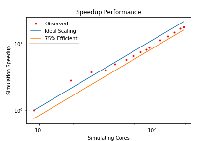
First of all, these strong-scaling results are shown as a log-log plot, while we used a semi-log plot thus far, so it will look slightly different (it is more common to use the semi-log plot that we have used before). But have a closer look at the measurements, what is going on with the second and third measurements? This is not a measurement error, and it is not the result of averaging measurements or manipulating them in some other way. The speed-up we are seeing is real.
But how can we get a speedup that is larger than the theoretical best performance? In other words, if we have, say, a speed up of 2.2 for 2 cores, then our efficiency, according to Eq.(15), is E=2.2/2 = 1.1 = 110%. We have an efficiency that is greater than 1, or 100%, something seems to be off here. But let’s look at our computer hardware a bit closer:
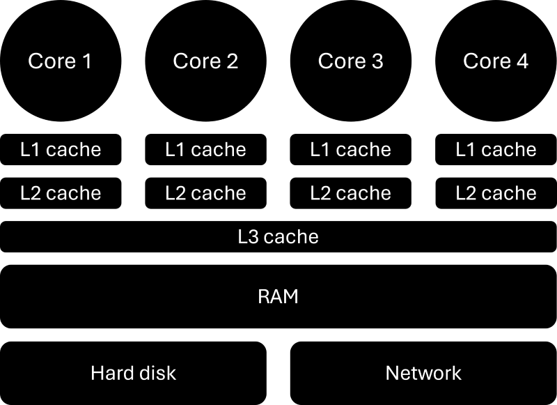
As we have discussed, a CPU consists of several cores, or processors, but they also have a number of caches, typically three levels. The L1 and L2 (level 1 and level 2) caches are sitting next to each core and are local to that core, but the L3 (level 3) cache is shared among all cores on the CPU. When data is required from main memory (RAM), the CPU will request the relevant data to be copied into the L3 cache. Each core will then take from that L3 cache what it needs and put that into its L2 and L1 cache.
The reason we do that is speed. The CPU is so fast that if we were to always read memory directly from main memory (RAM), it would take so long that most of the time the CPU would be waiting for memory. The solution is caches. It is the same reason we do grocery shopping. When we want to cook, we don’t go to the supermarket and buy the stuff we need, but rather get a bunch of ingredients upfront and then, when we want to use them, we go to the fridge and food cupboard and get what we need.
In this analogy, the supermarket is RAM, and our fridge/food cupboard is our cache. When we need memory, the CPU requests data and places it in the L3 cache so each core can use it, which is equivalent to us going to the supermarket and getting a bunch of things which we can store at home so they are there when we need them. While the supermarket has so much capacity that it has pretty much anything we could ever need, our fridge and food cupboard have limited space.
The trade-off, thus, is the capacity for access speed. I can get anything I want in the supermarket, but it will take time to get it. But if I can get what I need from my fridge or food cupboard, it is there, and access time is basically zero. The same is true for RAM and caches. Accessing memory from RAM is slow, but accessing memory from our caches is fast. In the case of L1 caches, it can be as little as a single clock cycle (which means our CPU has the data available when it needs it and doesn’t have to wait for it).
The following figure shows access times vs. capacity for different memory modules, which helps to illustrate this point. Note that these numbers are approximate, so the order of magnitude is more important than the absolute value.

The CPU will only work with registers, which are sitting next to each core. Their data is coming from the L1 cache, and so on. We can see that the smaller the memory modules are in capacity, the faster they can load memory. The reason is that memory needs to be indexed, which can take time. If you park your car in a parking area that takes 20 or 2000 cars, in which of these parking areas will you, on average, find your car quicker? The smaller the parking area, the faster the access time, and the same is true for memory.
So, how does all of this relate back to our strong scaling results? Well, let’s use the figure above and see what happens if our baseline simulation consumes 2 MB of storage. Arguably, this is a very small problem, but let’s go with this example. We run this example on 1 core and, because this problem is so small, it does fit entirely into our L3 cache. No need to go to main memory.
We now perform our strong scaling measuring campaign and realise that for 2 and 4 cores, we get an efficiency of more than 1, or 100%. The reason here is that we split our original 2 MB problem now amongst 2 and 4 processors. Thus, each processor will get a problem size that is now either 1 MB or 0.5 MB, respectively. Looking at our memory hierarchy above, we can see that this is now just about small enough so that the entire problem fits into the L2 cache.
Since the L2 cache has faster access times than the L3 cache, we do see a speed-up that goes beyond the predicted theoretical best. What we have to realise here is that the theoretical best performance was predicted based on the single-core simulation, which took place in the L3 cache. But once we break down our problem, eventually it will fit into smaller caches, where the theoretical best speed-up is different.
However, since we compare our results against the theoretical best based on the single core simulation, we can get efficiencies that are above 1, or 100%, i.e. we see speed-ups that go beyond what is theoretically possible. This behaviour is called superlinear scaling, or superscalability, and is just a consequence of our memory hierarchy.
Weak scaling
In strong scaling, we took a fixed problem size (e.g. the number of cells in the mesh) and measured the speed-up for an increasing number of processors. This meant that the problem size per processor was getting smaller and smaller as we increased the number of processors. In weak scaling, on the other hand, we keep the problem size per processor the same.
So, if we simulate a problem of 1 million cells on a single core, then, in weak scaling, we would have to use a problem size of 2 or 4 million if we measured their weak scaling for 2 or 4 processors, respectively. The question then becomes, why would we do that? If we keep the problem size the same per core, we would expect to see the same computational times, or not?
Let’s think about what happens when we increase the number of processors. Initially, we only use a single core. Even if we increase the number of cores to a handful, we are likely still on the same compute node. As we increase our number of cores, we start to use more than a single compute node. If we increase the number of cores even further, we will start to use compute nodes that are further apart in space.
At first, these compute nodes are within the same cabinet, but then, as we use more and more cabinets, our communication has to go through the network, which is now separated in space. The further apart these compute nodes are, the longer it takes to send data over the network.
Consider this: HPC clusters use optical (glass) fibres in their network. This allows them to send data at almost the speed of light, i.e. c=300,000,000\, m/s (approximately, let’s not split hairs). The speed at which data is sent depends on the refractive index, which is a ratio of how fast light travels in a medium compared to a vacuum. In glass, this value is about n=1.5 for visible light, meaning that a signal in optical glass fibres may travel at:
v=\frac{c}{n} = \frac{300,000,000}{1.5} = 200,000,000\,m/s\tag{16}This means that it takes the network about 1/200,000,000=5\,ns (nanoseconds) to send data for 1 metre through the network. Our CPU, in the meantime, is able to perform calculations according to its clock cycle, which is about 2-3 GHz on HPC clusters. This means it takes the CPU about 1/3,000,000,000=0.3\,ns to perform one operation. If two nodes are separated now by one metre, the CPU can perform 5/0.3\approx 16 operations while data is being sent over the network.
This does not include the time it takes to read data from RAM and put it onto the network, and write it back into RAM at its destination. What this calculation shows is that as our compute nodes are getting separated physically in space, the time it takes to send data becomes a bottleneck. Who would have thought that the speed of light is not fast enough for CFD applications!
Returning to our weak scaling problem, as we increase the number of cores, we don’t just increase the number of communications that need to happen, similar to strong scaling, but we also test how the additional distance in space affects the communication speed.
In general, when we try to benchmark our CFD applications, we perform a strong scaling analysis, and usually, we are happy with that. Weak scaling is not often done. You only really need weak scaling if you are targeting really large simulations (1000 cores or more, let’s say), but most of the time, this analysis will not give you any actionable insights to improve your parallel efficiency.
Weak scaling is usually much more important for those who maintain the HPC facilities and try to identify bottlenecks, or just to benchmark their system. If we performed two separate weak scaling tests on two different systems, we likely would get different results. In a sense, the weak scaling results are mostly influenced by the HPC system itself rather than our code.
Thus, if we wanted to improve our code, especially our parallel efficiency, we would perform a strong scaling analysis and try to improve our communications here. Any improvements made in strong scaling would also show in weak scaling, though the bottleneck in weak scaling would still be the system that we use.
Let’s look at another example, say we have to look at a simulation where we have kept the problem size the same. For the sake of argument, imagine we run a problem where the meh size is exactly 1 million cells per core, and we measure the computational time it takes as we add more and more cores, keeping the number of cells per core the same. Example measurements can be found in the table below:
| Number of cores (required nodes) | Measured time (in seconds) |
|---|---|
| 1 (1 node) | 0.58 |
| 2 (1 node) | 0.63 |
| 4 (1 node) | 0.72 |
| 8 (1 node) | 0.79 |
| 16 (1 node) | 0.89 |
| 32 (1 node) | 0.97 |
| 64 (2 nodes) | 1.03 |
| 128 (4 nodes) | 1.26 |
| 256 (8 nodes) | 2.41 |
| 512 (16 nodes) | 4.59 |
| 1024 (32 nodes) | 10.69 |
| 2048 (64 nodes) | 22.01 |
We can now compute the efficiency again, this time expressed as:
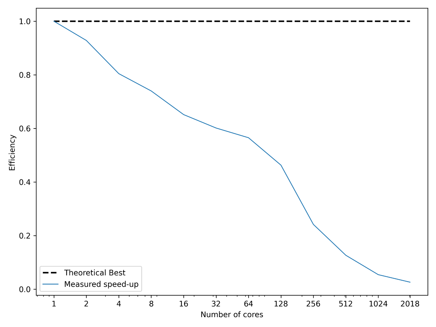
E(p, N)=\frac{T(1,N)}{T(p,N)}\tag{17}Thus, we take the time it took to run this simulation on one core (i.e. 0.58s) and compare that to subsequent simulations. In an ideal world, as the number of cores increases and the problem size per core remains the same, we would expect the computational time to be the same. While the computations don’t change, the time we have to wait for data will increase, and so we will see a departure from a 100% efficiency. This is shown in the following figure:
This is all there is to weak scaling, really. But one question is still open. After we have done our strong and weak scaling, how can we determine the number of cores to use that is optimal for our simulation? This is the question we seek an answer to in the next section.
The optimal number of cores for your simulation
Indeed, if we just did the strong and weak scaling to plot some fancy plots, we would have wasted quite a lot of computational resources for one figure. If this figure then never gets used, for example, in a publication, then what was the point of this exercise? Typically, we want to perform the strong scaling so we can compute an optimal problem size per core, that is, for how many cells per core do I still get a good speed up with a good parallel efficiency.
As we have seen both in the strong and weak scaling sections, it is impossible to get something with a parallel efficiency of 100%, unless we use a single core (at which point, we don’t have parallelism, so this is a pointless answer). So, first we have to settle on a level of parallel efficiency we are happy with, and then we can try to identify a suitable problem size per core.
A good rule of thumb is that 75% – 80% is an acceptable parallel efficiency, so when you perform your strong scaling, you look at which point you reach a value of 0.75 \ge E(p, N) \ge 0.8 and then find the number of cores and the problem size. Say you achieved this value with 8 cores and your problem size was 1 million cells. Then, you can compute the optimal problem size as:
N_{opt} = \frac{N}{p|_{0.75 \ge E(p,N) \ge 0.8}} = \frac{1,000,000\,cells}{8\,cores} = 125,000\frac{cells}{cores}
\tag{18}
Once you have performed this analysis, you have generalised your strong scaling results and extracted some actionable insights. If I come along and I want to use your code, and my simulation uses 15 million cells, then you can tell me that the optimal number of cores is 15,000,000/125,000=120. Except, it isn’t! The correct answer is either 64 or 128.
To understand that, let’s consider the HPC hardware. We have our different cabinets and compute nodes, and we need to connect them all together. What is the optimum way to connect them? Well, HPC interconnection is a topic in itself, but let’s just say that all of the common topologies we use, like the hypercube or Torus, require 2^m connections (where m is an integer). For example, if you follow the link to the hypercube, it will say:
“Hypercube interconnection network is formed by connecting N nodes that can be expressed as a power of 2. This means if the network has N nodes it can be expressed as:”
N=2^m\tag{19}Similar observations can be made for the Torus interconnect. Thus, if we have 2^m network links connecting different compute nodes together, then it would make sense to have 2^n cores to efficiently use this network (where n is an integer). If we use a number of cores that can not be expressed as 2^n, then we don’t utilise the network efficiently.
On the parallelisation side of things, there will be algorithms that expect us as well to use 2^n cores. Some algorithms are implemented in a way that expects either 2, 4, 8, 16, 32, … cores, so that it can always divide a problem into 2 and then distribute that amongst cores. If I have one computation and want to split it into 2, I get 2 sub-problems to solve. If I divide this again by 2, I get 4 sub-problems. Divide that again by 2, I get 8, and so on.
If I come now with 12 cores, then I cannot efficiently distribute that problem. Our parallelisation framework will be able to handle 12 cores, but it has to do some additional work, which slows us down. If we just come with 16 cores instead, we can nicely subdivide our problem into 16 sub-problems, which allows for fast execution.
Coming back to our example of me wanting to use your code with 15 million cells, the answer is not 120 cores, but rather 64 or 128, both of which can be computed with 2^n. In this case, I would probably select 128, as this is really close to 120 and 15,000,000/128\approx 117,000, so it is not miles away from the theoretical optimum (which will likely also contain some variance).
Thus, when we want to determine the optimal number of processors, this is the generalised approach:
- Perform strong scaling analysis of a problem size that is sufficiently large.
- Compute the parallel efficiency and identify the number of cores required to retain a 75% – 80% efficiency.
- Compute the optimal number of cores as we have done in Eq.(18). This will be your lower bound C_{lower}.
- Multiply the optimal number of cores by 2. This will be your upper bound C_{upper}
- Determine the value of n for which the following inequality is satisfied: C_{lower} \le C_{given} / 2^n \le C_{upper}. Here, C_{given} is the number of cells of the problem we are trying to solve.
- Calculate the number of cores as N_{cores} = 2^n.
You can do that, write your own calculator for that, or, shameless plug, use my browser extension, which has a parallel computation calculator that will do all of that for you. If you don’t want to use the calculator, or even write your own, here are some good default values:
- Assume that commercial CFD solvers will retain a parallel efficiency of about 75% – 80% for 50,000 – 100,000 cells per core.
- Assume that in-house (academic) codes or open-source CFD solvers, unless touched and optimised by some HPC wizard, retain a parallel efficiency of 75% – 80% for 100,000 – 200,000 cells per core.
If I leave this discussion here, someone will inevitably point out a flaw that I have used throughout my discussion up to this point. I have always been referring to our problem size as the number of cells in our simulation. However, the number of cells is not necessarily a good indicator of the amount of work we do. For example, the work done on a 4-million tetrahedral-dominant mesh and a 1-million polyhedral-dominant mesh may be the same.
In reality, the number of faces, not the number of cells, determines our computational cost (assuming we are using a finite volume method). So, if you just want to be that extra bit pedantic, or you are German, then use the number of faces, not the number of cells. I was thinking how I could show you why Germans are the way they are, I don’t think I can, but here is a good summary of German values …
The music is meh, but the lyrics are, well, I shall not spoil them. If you are interested, here is a somewhat decent translation. It really brings out that German arrogance that people in the world have come to love about us (I think …).
The reason we use the number of cells to determine the computational cost is due to historical reasons. When we started to do CFD in earnest around the 1950s, with pioneering work of Lax, Friedrichs, Harlow, Welch, all was done in 1D and 2D on structured grids. Since structured grids only allow for a single cell type, it doesn’t matter if we take the number of cells or the number of faces. The work will scale well with either metric.
Only once the finite volume method was introduced in 1971 by McDonald and, independently, in 1972 by MacCormack and Paullay, did we start to adopt new elements that could be treated by the finite volume method, including polygons (2D) and polyhedra (3D). Since polygons and polyhedra elements can have an arbitrary number of faces, using the number of cells is no longer a good indication for the computational work, as the finite volume method is face-based, that is, integrals/fluxes are evaluated at the faces.
Therefore, we ought to use the number of faces, and not the number of cells, when we talk about computational cost, but I suppose this is yet one more example of how CFD is full of wonderful inconsistencies.
People in the finite element community, however, have realised that the logic we are using is flawed, and so when they talk about problem sizes, they use the term degrees of freedom, which also accounts for the fact that you may have a different number of integration points per cell.
In any case, I have admitted the logical inconsistency, so you don’t have to tell me that I am wrong.
The roofline memory model
When we did our strong scaling analysis, we wanted to identify when our performance is dropping. We used the efficiency to guide us in this case, and we ended up with the smallest problem size per core that still gives us an acceptable parallel efficiency.
Let’s say after we have obtained this number, we realise that our code is just very slow, but we don’t know where this is coming from. So, we want to benchmark our code to identify the bottleneck, so that we know which part of the code we have to improve. This is where the roofline model comes in. Arguably, it is a simple model, and much more sophisticated models are available, but it helps us to identify which bottleneck we have, and we have two possible solutions. Either we are:
- Memory-bound
- Compute-bound
If we are compute-bound, it means that we are already utilising our CPU to its maximum capacity. We cannot squeeze more out of our CPU by giving it more work to do; if we wanted to get more performance, we would need to get a CPU with a faster clock cycle (i.e. get a CPU with more GHz).
If we are memory-bound, however, then our CPU is not getting enough data to operate on. Either the CPU is not doing enough with that data before it requests new data, or our memory supply is not optimised. Typically, we have enough data for the CPU to work on, so if we are memory-bound, it usually indicates that we are very inefficient with our memory access.
Let’s create an example to understand how memory access can cause a bottleneck and result in our application being memory-bound. Let’s say we want to perform a simple vector matrix multiplication. This is something we routinely do in our applications, and so you may have a few of these in your code as well. Let’s look at a very simple example:
#include <vector>

using MatrixType = std::vector<std::vector<double>>;
using VectorType = std::vector<double>;

int main() {
 int N = 1024;

 MatrixType A(N, std::vector<double>(N));
 VectorType x(N);
 VectorType b(N);

 // fill data for A, x, b. Not done here, a real application would do that.
 // ...

 // b = A * x
 for (int j = 0; j < N; ++j) {
 for (int i = 0; i < N; ++i) {
 b[i] += A[i][j] * x[j];
 }
 }

 return 0;
}I have defined two types on lines 3-4 to allow me to create a matrix (consisting of two std::vectors arranged as a 2D matrix) and a vector (consisting of a single std::vector). I use these types to create the matrix A and the two vectors x and b on lines 9-11, using the number of elements per row/column as defined by N (which would be, for example, the number of cells in our mesh).
On lines 17-21, I perform the vector matrix product, i.e. b = Ax. If your programming background is from Fortran, then this will look familiar to you. We have two loops, and we first loop over j (columns), and then over i (rows). The order in which we would access our matrix is shown in the following:
\begin{bmatrix}
1 & 4 & 7 \\[1em]
2 & 5 & 8 \\[1em]
3 & 6 & 9
\end{bmatrix}\tag{20}
Because we are accessing each column one after the other, we call this the column major ordering. But, we could have also reversed the loops and have:
for (int i = 0; i < N; ++i) {
 for (int j = 0; j < N; ++j) {
 b[i] += A[i][j] * x[j];
 }
}In this case, the matrix would be accessed in the following order:
\begin{bmatrix}
1 & 2 & 3 \\[1em]
4 & 5 & 6 \\[1em]
7 & 8 & 9
\end{bmatrix}\tag{21}
Because we are going through the matrix row by row, we call this the row-major ordering. The question is, which of these is better suited to compute the vector matrix product? It all depends on how C++ stores variables, and it does that in row-major order. To confirm this, we could benchmark both vector matrix multiplications and see which is faster. I have done just that and used Google Benchmark to time both versions. There is a handy website that helps us do that called QuickBench, which I have used.
The result from this comparison is shown below:
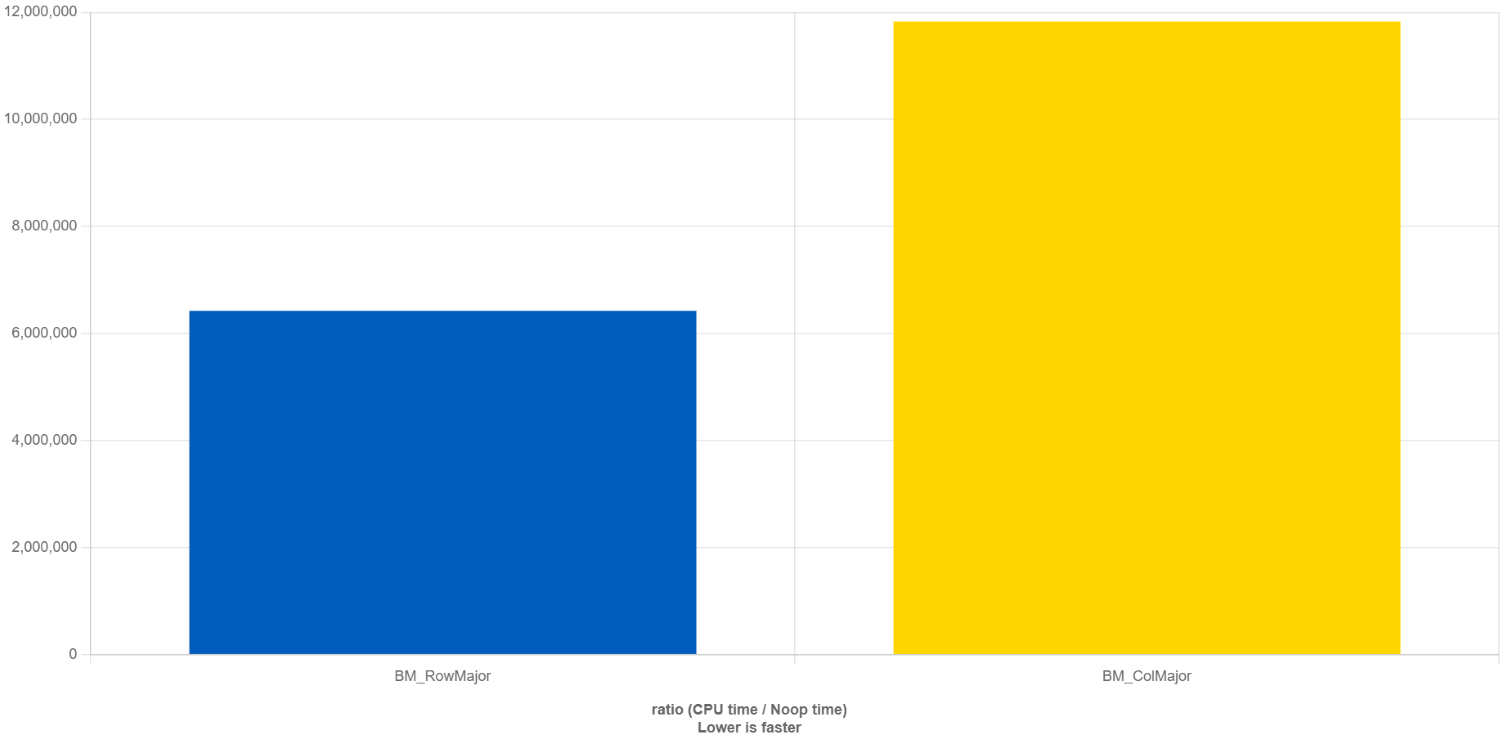
What QuickBench is doing is to compute the time it takes to perform a no-operation (noop, great name!) function call (i.e. calling a function that doesn’t do anything), and then comparing that time against the time it takes to compute our row major and column major matrix vector multiplication, so the y-axis is a non-dimensional unit of time.
Thus, the smaller the bar, the shorter the execution time. We can see that the row-major matrix vector multiplication on the left (blue bar) takes about 1.8 times less time to compute than the column-major matrix vector multiplication. What we learn from this is that we should always use i,j,k loop variables, not k,j,i when looping over multidimensional arrays. But why?
Remember when we talked about the memory hierarchy, I said that whenever the CPU needs new data in its registers to perform a computation, it will request that data from the L1 cache. If it is available, then it can load that data quickly and continue its computations; otherwise, it will have to wait for the L1 cache to request the data from the L2 cache. If it is there, the L1 cache will get this data quickly; if it is not, the L2 cache needs to request it from the L3 cache, and the L3 cache may have to go to RAM to get the data.
Whenever the CPU request the next element in an array (be it a 1D vector or a multidimensional array), we don’t just load a single element into our caches, but rather, we fill our caches with as much memory as possible so that when we request the next element, it will already be available. Whenever we request data, and it is already available in our cache, then we have a cache hit. If it is not available, we have a cache miss. Whenever we have a cache miss, we need to go back to the next cache or RAM to get additional data.
Getting the data will take time, and so we want to minimise cache misses as much as possible. The way to do that is to align our memory access with the way C++ stores its data. Let’s take a simple example and say that we have the following matrix:
\begin{bmatrix}
1 & -1 & 2 \\[1em]
7 & 4 & -4 \\[1em]
5 & -3 & -2
\end{bmatrix}\tag{22}
Let’s say that our CPU can hold 3 doubles in their register. With a row major memory access, we would first load 1,\, -1,\, 2 into our register. If we now also had the vector x loaded into another register, then we could compute the first entry into our b vector as 1x_0 -1x_1 + 2x_2. Since both the first row of our matrix and the vector x are in our registers, we were able to perform this operation without going back to our caches to request additional data.
To complete the first row in our vector matrix multiplication, we have to, yet again, request a new line column from our matrix, now 2,\, -4,\, -2, and we can calculate 2x_2. We can add that to the previous accumulated sum. Thus, to compute the first row, we had 3 memory loading instructions for our matrix using column-major memory access compared to 1 memory loading instruction for our row-major memory access.
If you continue this for the second and third row, you will end up with 3 memory load instructions for row-major memory access and 9 memory load instructions for column-major memory access. Memory is expensive, even with a clever cache hierarchy, and for that reason, we see that column-major memory access is 1.8 times slower than row-major memory access in our benchmark performed above.
So, the question then is, how do we know if our application is already saturated and using all the available power from our CPU (i.e. we have a compute-bound problem), or if we are having bad memory access and need to think about how to optimise this? This is where the roofline model comes in.
The roofline model defines two properties: the theoretical max performance of our CPU, measured in GFLOPs (giga floating point operations per second), that is, how many billion arithmetic operations can be performed on floating point numbers per second, and the operational intensity, measured in FLOPs/byte.
We need to define two units here. First, we have to consider the work performed. This is given the letter W, and this would be related to the work the CPU is doing, typically, how many floating point numbers it can work on per second. For this reason, we typically use GFLOPs when plotting the roofline model.
The second unit we need to look at is the memory traffic Q, and it measures how much data was requested by the CPU to perform its work W. With both of these numbers defined, we can compute the arithmetic intensity I as:
I=\frac{W}{Q}\tag{23}
This gives us a ratio, which essentially tells us how much data we need to perform a given number of operations. For example, let’s look at the following two operations:
a = a^2 + a \\[1em]
b = c * d\tag{24}
In the first example, we need to load 1 floating point value $a$ to perform two floating point operations, and then we need to store one floating point number. Let’s say that $a$ is a “`float“`, which typically takes 4 bytes of storage. Then, we can say that we have 1 load and 1 store operation, which takes 8 bytes in total. We have 2 floating point operations, i.e. $a^2$ and then the addition of $a$ with that result. Then, our arithmetic intensity would be:
I=\frac{W}{Q}=\frac{2}{8} = 0.25\,\, FLOPS/Byte \tag{25}
Let’s look at the second example. We have two load instructions of $c$ and $d$, and one store instruction for $b$. We have one floating point operation, i.e. $c \cdot d$, so we have an arithmetic intensity of:
I=\frac{W}{Q}=\frac{1}{12} = 0.08\dot{3}\,\, FLOPS/Byte \tag{26}
Now we need to look at the peak bandwidth of our system. The peak bandwidth is the maximum memory transfer rate between the CPU and memory. It is usually measured in GB/s. The easiest way to figure that out is to use a benchmark tool that will run some calculations, where the amount of memory to be transferred is known, so measuring the time it takes to transfer that data can be used to compute the bandwidth. A common benchmark is the [STREAM benchmark](https://github.com/jeffhammond/STREAM), and on my PC, I am getting values between 35 – 50 GB/s, depending on the operation.
Knowing this value, we can now compute the performance as the product of the peak bandwidth, let’s call that $\beta$, and the arithmetic intensity $I$. In our examples above, we would get the following performance:
P = \beta\cdot I = 50\frac{GB}{s}\cdot 0.25\frac{FLOPS}{Byte} = 12.5\frac{GFLOPS}{s}\\[1em]
P = \beta\cdot I = 50\frac{GB}{s}\cdot 0.08\dot{3}\frac{FLOPS}{Byte} = 4.1\dot{6}\frac{GFLOPS}{s}\tag{27}
Later, after becoming a lecturer and seeing what effort goes into ensuring the highest ranking in the QS tables (with their own working groups within universities), I realised that the ranking correlates to academic excellence just as much as the import of fresh lemon correlates to road accident fatality rates. We can even plot this:
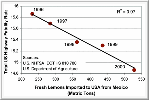
Sure, there is a correlation, but if you think about this correlation for a second, you realise that this correlation is accidental. Of course it is. This is an example of p-hacking, an art of scientifically proving that there is a mathematical correlation which does not exist in reality.
I have found that some universities will be at the top on merit; they are just excellent. Others are at the top because they know how to p-hack their way to the top. What I find disturbing in these rankings is that output and impact are the driving metrics. One could argue that academic conduct should be part of it as well, i.e., excellence in supervision, training new talent (students, researchers, etc.).
If we were to include this, arguably, difficult-to-measure quantity in the ranking as well, we would see a very different ranking. Top universities are not known for getting their by treating their students and researchers with respect; I should know, I had to sign a contract whose terms, from an ethical research point of view, were questionable, to say the least. Well, this is my experience, yours may differ …
Be that as it may, I was actually quite optimistic when I started at Imperial College. The year was 2013, and I met my two supervisors who would guide me through my research on Direct Numerical Simulations. Both of them were Greek, and I was German. Oh boy, did they have a field trip with me.
While the Greek debt crisis never really concerned me, all of a sudden, I felt the nation of Greece was looking for payback, and I was the recipient, on behalf of the German government. Here are just a few of the things they told my peers and me (I was part of a larger research group):
- “You are viewed as the golden boys (whatever that meant, we were a mix of male and female researchers), you can’t just take holidays whenever you want”
- “For the amount of money we pay you, you are not allowed to make these mistakes”
In other words, if you take holidays and you continue to make mistakes, then you can’t produce papers every other month. Research papers in good journals means research reputation and thus a higher ranking in the QS tables. This is a great system, which certainly isn’t broken.
But let’s look at these statements they made again. The first statement was told to one of my friends, who asked for some time off to go back to his home country to attend his grandfather’s funeral, who had passed away just a few days prior. In the end, they settled on “I can’t deny your request, but I am encouraging you not to go”.
Great human skills on display, imagine the scientific tragedy by having to delay your paper submission by one week. I’m sure researchers around the world couldn’t wait for more papers from us and spamming their F5 key, in the hope of being the first to read our prestigious research. I’m sure my supervisors actually believed this to be the case.
Or what about the second statement, you know, the one about not being allowed to make any mistakes. That was a meeting I had with both of my Greek supervisors, after I showed them the results of my code. There were some inconsistencies, but now I know how they came about. Back then, I did not, and so my supervisor asked me about my implementation and slayed me for how I implemented the Runge-Kutta time integration.
It wasn’t a comfortable meeting, to put it mildly, but for exactly that reason, it is a meeting that is still very vivid in my mind. I still remember exactly the issue my supervisor had with my implementation, and of course, if your supervisor tells you you messed up, you shut up, go back, and fix it. At least that was what I thought based on the impressions they gave me.
The problem was, my implementation was correct, and my supervisor did not understand himself how to implement the Runge-Kutta method correctly, it seemed. I even pointed out his flaws in our meeting but he was not in a mood to be corrected. He played the “I am the supervisor, and not just any supervisor, I work at Imperial College (here we go again), you are just the stupid researcher. If I say it is correct, it is correct” card.
After reading about it a few more times, looking at other people’s codes, and consulting with authorities who I knew would be able to tell me if I was right or wrong, I realised that I was, indeed, right all along, and my supervisor was wrong. So much for academic excellence.
The other problem was that I had to use his research code, written in good old Fortran 66. When the others and I in our research group started to use his code, we were told that half of the input parameters would not have any effect on the solution (i.e. they are there, but they are not yet implemented). The solver only understood a particular mesh file format, but there was no mesh generator available to generate meshes for the solver (and so we had to buy a license for ICEM-CFD to be able to use the solver).
On my PC, the solver would always crash after about 784 timesteps. My supervisor’s response, “I don’t know why this is happening, but it should work”, which very quickly became his catchphrase. We ran his solver through valgrind and saw that a memory leak was present, but despite the evidence, he refused to accept that his solver was not working (2 weeks later, we received an email from him with a zip file attached that fixed the memory leak that didn’t exist).
The solver had two numerical schemes implemented, the first-order upwind scheme, and the second-order central scheme. The first-order upwind scheme is stable, while the central scheme is uncondiotionally unstable.
In one of my first meetings, I was asked to produce some results to show that I can use the solver, and so I used the first-order upwind scheme. That triggered my supervisor, who lectured me on how first-order schemes are not good for scale-resolving turbulence simulations. Well, obviously, but the alternative was an unconditionally unstable scheme.
Again, putting his full ignorance on display, he told me to go back and run the same case with the central scheme. I did, and, as expected, the simulation blew up, and my contours were a collection of random noise. I showed it to my supervisor and thought this would put things to rest, but honestly, this is what he said: “Brilliant, you have successfully captured turbulence”.
Looking at the contour plot (and I really should have kept that image …), it was very clear that I did not generate turbulence but rather numerical instabilities. Sure, they look similar to turbulence, but I mean, there were so many tell-tale signs that it wasn’t turbulence.
For starters, I was putting velocity in with, say, 1 m/s, but then I would get turbulent eddies that had 5 times the velocity, all close to the inlet, without any obstacles in their way. Sure, it looked turbulent, but also not physical. I mean, the fact that this was a 2D simulation within a channel, the Reynolds number was about 100, and the grid wasn’t able to resolve any turbulent scales should have been a pretty big hint, but again, I was told I was wrong and needed to fix it.
My solution was to implement a higher-order scheme, so we would avoid the first-order upwind issue while gaining accuracy, but that was seen as wasted time. My time was better spent obtaining results my supervisor would sign off on (which I knew were wrong) and publishing these in reputable journals, essentially attaching my name to these physically incorrect results. I knew that any reviewer would see through these instantly and call me out for them, and I had a feeling I knew how my supervisor would react.
I was at my wits’ end and didn’t know how to really get out of the corner my supervisor put me in, and so I pulled the emergency brake, handed in my notice and left. Looking back, that was one of the best decisions I have made.
But, there is a point here, and I realise I have spent much more time on my Imperial College drama than was perhaps necessary. When I (and my peers) were running our supervisor’s solver on our internal HPC cluster, we were quickly contacted by the HPC admin and effectively got a soft ban on using the system. They said that all of our accounts were now limited to a certain number of cores. I don’t remember the exact number, but it was around 100 cores, definitely not enough for the Direct Numerical Simulations we wanted to perform.
The HPC team reviewed the scaling results of our supervisor’s code, and seeing those results was reason enough to enact the ban on using more cores. It was seen as electricity waste. Let’s look at the reasons.
First of all, the communications weren’t done very well, and a lot of time was wasted here. Some effort went into optimising the communications, and we need to look at the communications and their bottlenecks before we can understand this problem better. We’ll do that in just a bit when talking about MPI. That was just one issue, though.
The other issue was the load balancing. Our code was just horrible at assigning work to other cores, and thus, we needed a new and better domain decomposition approach. Domain decomposition was done in the following way: Decide how many times you want to cut the mesh in the x, y, and z directions. This will give you the number of regions in the x, y, and z directions, and their product is the number of sub-domains and cores we need to run the simulation. Let’s look at an example:
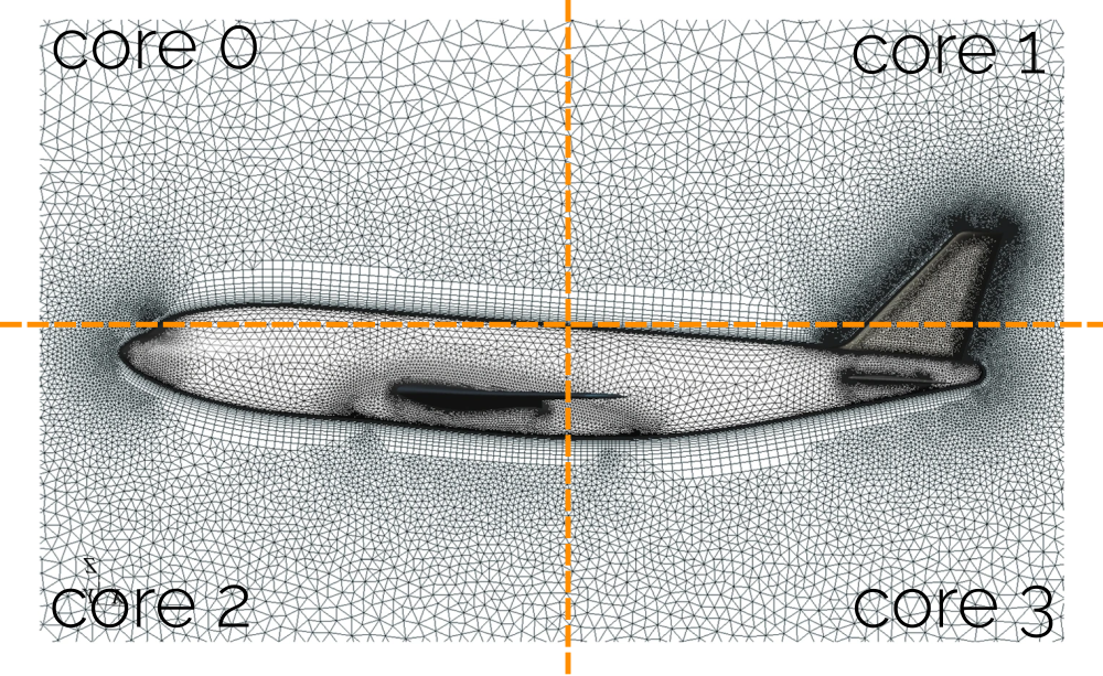
Here, we have decided that we will cut the domain once in the horizontal direction and once in the vertical direction. This will yield 2 regions in each direction, and so the number of sub-domains here is 2\cdot 2=4. This is what we can see in the figure above as well. Now, it doesn’t take an Imperial College graduate to realise that this is perhaps not the best way of splitting work (or sub-domains).
How can we ensure that each processor is getting the same number of cells? Well, we can’t! We simply divide our domain into equal geometric chunks and hope that all will have an equal number of cells per sub-domain. And, as we all know, good science starts with a healthy portion of hope and belief. I refer to this approach as the simple or naive domain decomposition approach. It works well on Cartesian grids, or on a whiteboard in the classroom, but not in reality for even slightly more complex geometries.
So, I worked on writing a new domain decomposition approach, where the number of cells per sub-domain would be taken into account. I also exploited the fact that we were only using structured grids for channel flows, so I could simplify my domain decomposition application. This is a sketch of what I essentially did:
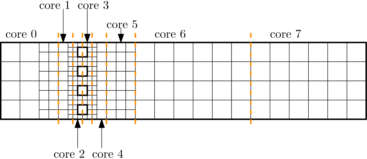
First, I would count how many cells there are in the mesh. In the example above, we have 192 cells. Then, I decide how many cores I want to use. In the example above, I am using 8 cores. Then I can compute that I will need 192/8=24 cells per core to achieve good load balancing. So, I start at the left, I count how many cells are in the first layer, and if there are fewer than 24 cells, then I go to the next layer.
Once I have exactly 24 cells or more in my sub-domain, I insert a slice and say all the cells to the left are now part of the first sub-domain. I continue going through the mesh and check where I should place my next slices. In this way, I approximately have the same number of cells per sub-domain, while also somewhat minimising the inter-processor boundaries.
There are better ways to deal with this issue, but using this domain decomposition approach, along with the improvements we saw in the communications, allowed us to get much better strong scaling results, and we were taken off the naughty list and allowed to run our simulations on the cluster again.
Before we finish this section, let’s look at how domain decomposition is done in OpenFOAM. It actually has a few different domain decomposition approaches implemented, such as the hierarchical one, which is doing essentially what I have implemented for our channel flow example. It allows the user to specify how many sub-domains should be created in the x, y, and z directions, and OpenFOAM will try to cut the domain in such a way that the number of cells per region is approximately the same.
There is one more domain decomposition approach, which is simply called “simple”. An example of that can be found in the periodic hill case. This is working as we have discussed before, i.e. we tell OpenFOAM how many sub-domains we want in the x, y, and z direction, which are then split into geometrically equal portions, without any considerations given to the number of cells per sub-domain.
My memory may serve me badly, but I have the feeling that the simple domain decomposition was used quite a bit in early tutorials, which now seem to have switched to hierarchical. I just wonder, is it any surprise that OpenFOAM has its origin at Imperial College? This poor domain decomposition approach seems to run in the family. (OK, I stop now …)
Using space-filling curves
To be honest, this is probably the first, and probably also the last time you hear about space-filling curves in the context of domain decomposition approaches. That doesn’t mean they are not good, quite on the contrary, space-filling curves are easy to construct, dividing a domain into sub-domains with the same number of cells per sub-domain is even simpler, and we do get a quite good ratio of cells per sub-domain to inter-processor boundaries.
They really are something magical, at least to me, but that is mostly my Stockholm syndrome speaking. During COVID-19, we all did weird stuff, didn’t we? For me, it was the summer of 2020 that stands out the most. Being on paid furlough by the university, with no kids yet to look after, and the Kim dynasty being busy with K-dramas, I had some time on my hands and so decided to get lost in the wonderful world of Peano and Hilbert space-filling curves.
Someone mentioned to me that their in-house solver used space-filling curves as their domain decomposition approach, and naturally, as a professional domain decomposition developer myself, I was instantly hooked, but I had no idea what these space-filling curves were. So I asked, “What are these space-filling curves”? He responded, “I have no idea, mate”. Great … So I looked for help, and spent the summer of 2020 with Michael Bader in bed (with his book, I should clarify. Boy, this is going to be awkward when Frau Bader is reading this …)
So why are these wonderful objects not used more commonly, at least in the field of CFD? Well, it always comes down to the non-linear term and turbulence; the two things structural (FEA) people fear more than the Greeks fear the Germans. Once we understand space-filling curves better, I will show you their Achilles’ heel and why we don’t use them, especially since better alternatives are available (discussed in the next section).
But before you say “OK, I don’t need to hear more, I’ll go straight to the next section”, let me indulge you a bit in the fascinating world of space-filling curves. You’ll learn something you had no idea you needed to know, and you probably will forget most of it, yet it is somehow incredibly satisfying to learn. I know, I make a horrible salesman, I guess there is a reason why I work in academia …
First, we need to learn about turtle graphics. Turtle graphics consists of a turtle, which can either move forward, turn left, or turn right, and we can specify the turning angle. The turtle can also draw its path, so we can follow its trajectory. Take a look at the following two examples:

On the left, we start at the bottom left, and our initial direction is to the right (you could say, in the positive x direction). We define our forward direction as F, which means that our turtle is moving from one cell to the next in the current direction of travel. We further define turns to the left (counter-clockwise) as - and turns to the right (clockwise) as +. Each turn will be exactly 90 degrees. With a starting position and a starting direction, we can now define the steps the turtle makes for the left example as:
FF-F-F+FF+FF\tag{28}For the example on the right, we start now at the bottom right and define our initial starting direction in the negative x direction. With that in mind, we can define the path of the turtle as:
FFF+F+FFF-F-FFF+F+FFF\tag{29}We say that the path travelled by the turtle on the left is not a space-filling curve, as it has not gone through each cell. The turtle on the right, however, does produce a space-filling curve, as it has travelled through all cells. There are many ways in which we can construct a space-filling curve, but some will have better properties than others, and we will see that in a second.
But before that, we have to talk about the Lindenmayer system, usually abbreviated as just an L-system. Here is the Wikipedia definition of the L-system:
An L-system or Lindenmayer system is a parallel rewriting system and a type of formal grammar. An L-system consists of an alphabet of symbols that can be used to make strings, a collection of production rules that expand each symbol into some larger string of symbols, an initial “axiom” string from which to begin construction, and a mechanism for translating the generated strings into geometric structures.
If you understand a word of it, congratulations, I don’t (and keep in mind that I already know what an L-system is). There is a simple test you can do to see if you understand the L-system from the introductory paragraph on Wikipedia. The L-system was originally developed to describe the growth of bacteria and branching structures like algae. If you think this makes sense, then you are the clever one. But I am dumb and need things explained to me like I am 5 years old, so allow me to offer my explanation as well.
We already looked at a complete example of an L-system: our turtle graphics. An L-system consists of 4 aspects, which formalise the path of the turtle, the growth of bacteria or algae, or other branching structures. This is essentially the grammar that was mentioned in the definition above. These 4 aspects are:
- Variables
- Constants
- Axiom
- Rules
Let’s apply that to our turtle example. We didn’t have any variables in our system, and we will need a bit of explaining before we understand what variables are in the context of an L-system. The constants we had were -, +, i.e. for turning, and F, for moving forward.
The Axiom, sometimes also called the starter or initiator, essentially tells us our initial condition, for example, a starting direction, but more commonly, they refer to a starting rule, which brings me to the final point. Rules define how branching structures develop, or, in our example, how the turtle is moving. Let us write out the L-system for our first turtle example in full:
- Variables: None
- Constants: F, +, -
- Axiom: F
- Rules: F \rightarrow FF-F-F+FF+FF
So far, so good, but we rarely come up with systems in mathematics without some form of generalisation. So far, I have only said that L-systems are used to describe the path of a turtle, but I also mentioned that they can be used for branching structures. If you think about branching structures, especially in a mathematical sense, you may be thinking about fractals, and you would be right. Probably the most famous fractal is the Mandelbrot set, shown in the following:

So, the L-system helps us describe branching, or fractal structures. Take an example of some simple shapes shown in the figure below, we can branch these structures by creating the same base shape (shown on the left) with smaller elements of itself. So, we can also say that our branching structures, or fractals, are self-similar.
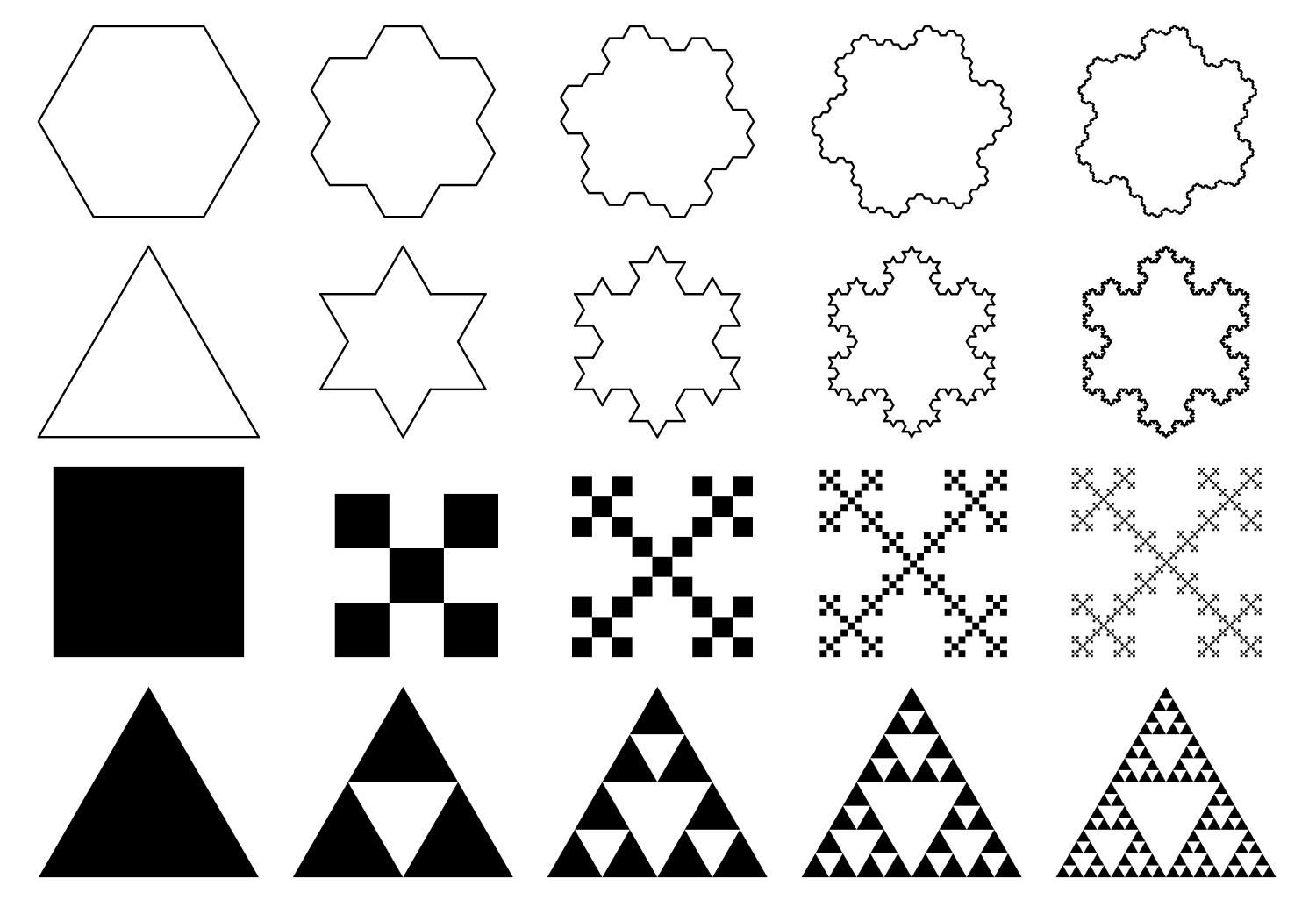
Once we have replaced the original shape with smaller elements of itself, we can replace these elements with smaller elements again, and this can be repeated until infinity, and the same principle was used to generate the animated GIF shown previously.
Ok, we are almost there, so now we can apply this thinking to space-filling curves, and we can see why this becomes important. The following figure shows two special kinds of space-filling curves: the Hilbert curve and the Peano curve.
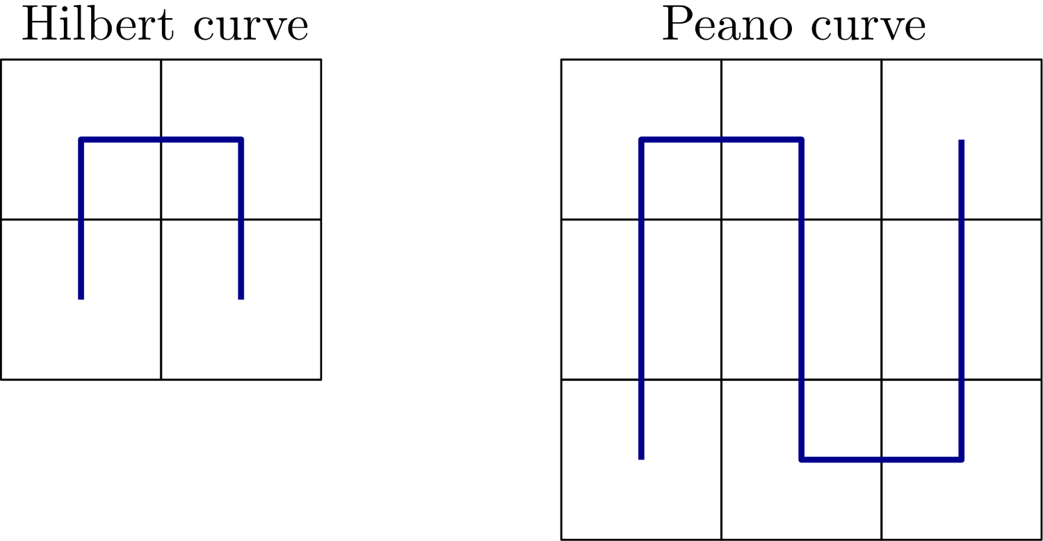
Yes, people have gotten fame for drawing curves like these in the past, different times, I suppose. But in all seriousness, usually it is difficult to appreciate the complexity behind an elegant solution that generalises to something as simple as the Peano and Hilbert curves.
Both of these curves are excellent for traversing a computational mesh and going through each cell. They do that by applying the same principles of fractals we have seen above. Let’s take the Hilbert curve as an example. In the figure above, we can say that the Hilbert curve currently goes through a 4-cell mesh. If we apply some mesh refinement, by halving the distance in x and y, for example, we can create a finer grid. In a sense, we have applied fractal thinking to mesh generation.
We can do the same with our space-filling curve as well, as shown in the following:
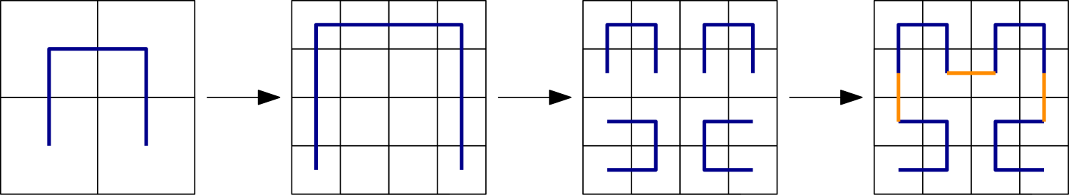
Here, we replace the original Hilbert space-filling curve with its fractal representation. Doing that means that we still cover the entire mesh. I have connected the individual Hilbert curves with an orange line to show that this space-filling curve is continuous. I was mocking Hilbert for making his name on a simple geometry curve, but in reality, his curve is not just space-filling, but also continuous, and that is a restriction on our set of curves which is far more difficult to prove mathematically.
So the question is, how can we generalise this using the L-system? The key is to introduce variables. Let’s write out the L-system for a Hilbert space-filling curve, and then we’ll discuss it:
- Variables: A, B
- Constants: F, +, -
- Axioms: A
- Rules:
– A \rightarrow +BF−AFA−FB+
– B \rightarrow −AF+BFB+FA−
OK, let’s start with what is simple. The constants are the same as in our turtle graphic example. To construct a space-filling Hilbert curve, well, we could get away with the definition of F\rightarrow F+F+F, right? At least if we look at the first iteration of the Hilbert curve, i.e. the left-most curve in the previous figure, then this rule would be sufficient to construct such a space-filling Hilbert curve. But, this system would not generalise to larger meshes (i.e. mesh refinement, as seen on the right of the figure).
So, we introduce variables, and it is the variables which provide us with the power of fractals. Let me give you an analogy. If we want to compute the Fibonacci sequence, we can do that with the following recursive equation:
F_i = F_{i-1} + F_{i-2}\quad \forall\, i\ge 2 \tag{30}We require that i is not smaller than 2, and as long as that is the case, and we use the initial data F_0=0 and F_1=1, we can compute any Fibonacci number based on this recursive equation.
With space-filling curves, it is sort of the same idea. If we look at the rules, we see that both A and B are defined recursively. The key to understanding this rule is that we don’t draw variables; we only draw constants according to our L-system. But how do we deal with A and B then?
Well, we first need to define how often we want to refine our Hilbert curve. In the figure above, we were drawing the original Hilbert curve on the left. So, this curve is said to be at iteration zero (no refinement done to the original curve). But, to its right, the Hilbert curve was refined once, and so we say that this is the first iteration of the Hilbert curve. If we refine the mesh further and use a further refined Hilbert curve, then we get the second, third, fourth, … iteration of the Hilbert curve.
For our rules in the L-system, it means that we have to apply the number of iterations to the rules, i.e. substitute A and B into themselves. Once we have done that for all iterations, we are done. At that point, we simply remove (or ignore) any variables, and only draw the path according to F, +, and - instructions. Let’s show that for iterations 0 and 1.
For iteration 0, we said we don’t need to substitute anything, and so we can simply remove all occurrences of A and B from our rules. This gives us:
- Iteration 0:
– The rule for A was: A \rightarrow +BF−AFA−FB+
– The drawing instructions for A become A \rightarrow F−F−F
– The rule for B was: B \rightarrow −AF+BFB+FA−
– The drawing instructions for B become A \rightarrow F+F+F
Since our axiom (starting point) for the Hilbert curve is A, and in the zeroth iteration, A does not depend on B, we can ignore B in the zeroth iteration. But, we see one important detail here, and the reason why we have both A and B defined: A is constructing the Hilbert curve in a counterclockwise direction, while B is defining it in a clockwise direction. We need that to be able to change directions; otherwise, we would not be able to construct a continuous space-filling curve.
Try to draw both A and B on paper; once you do, the system will make sense. The zeroth iteration is something you may be able to do in your head, but let’s look at the first iteration and see how this is done. Remember, we have to insert A and B into itself however many iterations we have. So, in our case, we have the first iteration and so have to substitute A and B once into itself. This results in:
- Iteration 1:
– The rule for A was: A \rightarrow +BF−AFA−FB+
– The rule for B was: B \rightarrow −AF+BFB+FA−
– Inserting A and B once into itself results in: A \rightarrow +(−AF+BFB+FA−)F−(+BF−AFA−FB+)F(+BF−AFA−FB+)−F(−AF+BFB+FA−)+
– Inserting A and B once into itself results in: B \rightarrow −(+BF−AFA−FB+)F+(−AF+BFB+FA−)F(−AF+BFB+FA−)+F(+BF−AFA−FB+)−
Now, we can again either remove or ignore any occurrences of A and B to get the drawing instructions. This results in:
A \rightarrow +(−AF+BFB+FA−)F−(+BF−AFA−FB+)F(+BF−AFA−FB+)−F(−AF+BFB+FA−)+ \\[1em]
A \rightarrow +(−F+F+F−)F−(+F−F−F+)F(+F−F−F+)−F(−F+F+F−)+ \\[1em]
A \rightarrow +−F+F+F−F−+F−F−F+F+F−F−F+−F−F+F+F−+ \\[1em]
A \rightarrow F+F+F−FF−F−F+F+F−F−FF−F+F+F\tag{31}
For B, we get:
B \rightarrow −(+BF−AFA−FB+)F+(−AF+BFB+FA−)F(−AF+BFB+FA−)+F(+BF−AFA−FB+)− \\[1em]
B \rightarrow −(+F−F−F+)F+(−F+F+F−)F(−F+F+F−)+F(+F−F−F+)− \\[1em]
B \rightarrow −+F−F−F+F+−F+F+F−F−F+F+F−+F+F−F−F+− \\[1em]
B \rightarrow F−F−F+FF+F+F−F−F+F+FF+F−F−F\tag{32}
Here, I have done the following things: first, I have removed all occurrences of A and B. Then, I have removed the parentheses, which were only there to help us see where we have inserted A and B into themselves. We end up with a few instructions that cancel each other out. For example, we get a few +- and -+ instructions, which basically state “turn clockwise by 90 degrees, then turn counterclockwise by 90 degrees”, and vice versa. So we can ignore those instructions as well.
What we end up with is again a system that only depends on F, +, and -. We also see that we sometimes get F twice in a row. If that is the case, just draw two lines, both of the same length as any previous line you drew. To make this clear, the following figure shows how the first iteration of the Hilbert curve looks for A and B:
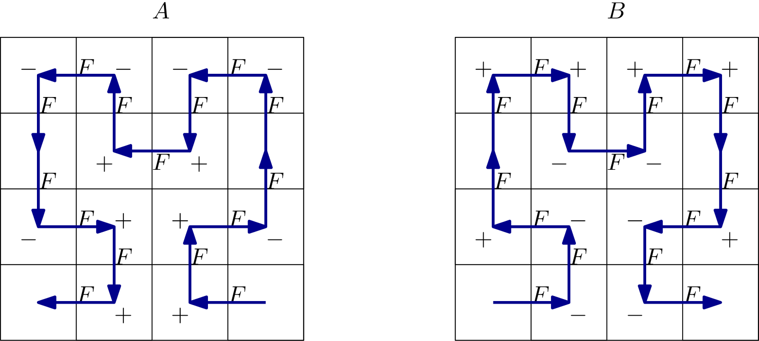
As we can see, A and B produce the same curve; they are just a mirror image of each other. You might be wondering how I determined the starting direction. Well, I picked one at random. The shape will be rotated by 90/180/270 degrees if you pick another direction, and as we will see in a second, regardless of the initial starting direction we pick, we still get a space-filling curve, no matter what.
Based on the L-system, we can now divide our mesh more and more, and then we have to keep fractalising (probably not a word) our Hilbertious curves (definitely not a word). And, because I am a sucker for space-filling curves, of course, I have written a Python script to do that. Here are the first 5 iterations of the Hilbert curve:
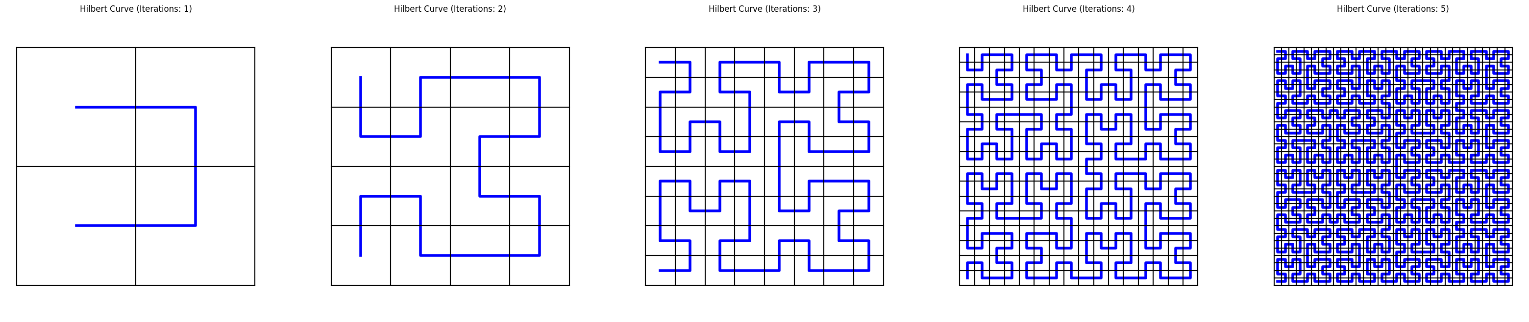
If you want to test your knowledge now, here is the L-system for the Peano curve:
- Variables: A, B
- Constants: F, +, -
- Axioms: A
- Rules:
– A \rightarrow AFBFA+F+BFAFB−F−AFBFA
– B \rightarrow BFAFB−F−AFBFA+F+BFAFB
I have implemented that as well in my Python script, and the first 5 iterations for it are shown in the following as well:
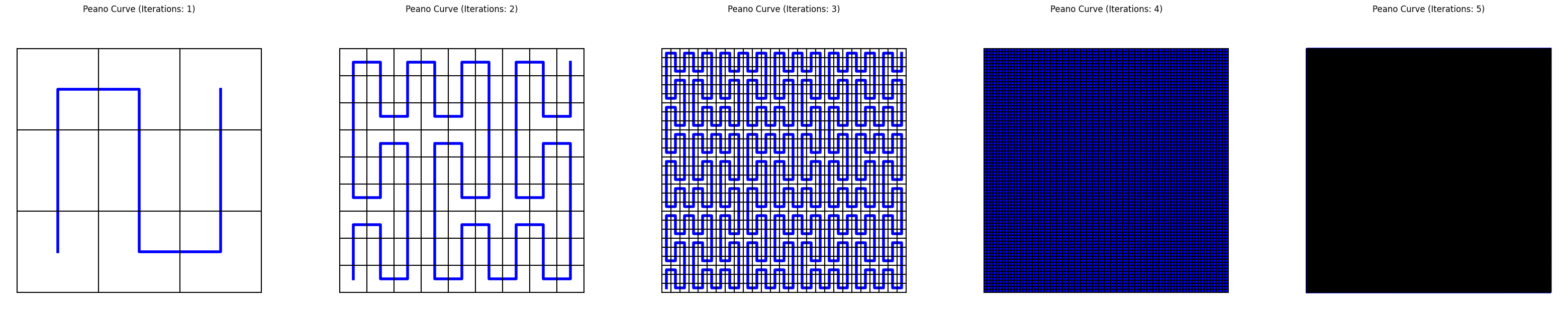
OK, we went quite far without talking about domain decomposition. So here it comes. We know how long our Hilbert or Peano space-filling curves are. Every time we draw a line with an F instruction, we have just extended the curve by 1. So, for example, in the zeroth iteration of the Hilbert curve, the curve is 3 units long, while the Peano curve is 8 units long. In the first iteration, the Hilbert curve is 15 units long, while the Peano curve is 80 units long.
If we compare that to the number of cells, then we see that in the zeroth iteration, we have 4 cells for the Hilbert curve and 9 cells for the Peano curve. For the first iteration, this increases to 16 and 81 cells, respectively. Comparing that with the length of each respective curve, we see that the connection between the number of cells and the line segments (LS) of each space-filling curve is:
N_{cells} = N_{LS} + 1\tag{33}Another property is that space-filling curves are localised. That means they fill up one area entirely before they move to another area. Both of these properties make space-filling curves ideal domain decomposition tools!
We take the number of line segments and divide it by the number of processors. This will give us the number of cells per sub-domain. All we have to do now is go along the space-filling curve and flag these cells, as well as count them, until we reach the number of cells required per sub-domain. All of the cells we have flagged will now be part of that sub-domain. We then continue to flag the next set of cells, which will be part of the next sub-domain, and again, we do that until we have reached the required number of cells per sub-domain.
Because space-filling curves are local, i.e. they try to fill up the space in one area before expanding, they will also give us a pretty good inter-processor boundary distribution, i.e. one where we minimise the number of cells in the inter-process boundaries per sub-domain. It isn’t perfect, but considering that we don’t have to spend any thought on it, it is pretty decent.
So, let’s do that for our Hilbert and Peano space-filling curves. In the following, I am dividing three iterations of each curve into 16 sub-domains so I can solve each with 16 cores. Each sub-domain, or rather, each curve per sub-domain, is now being plotted with a different colour so we can see which cells belong to which sub-domain. Also, the space-filling curve is no longer continuous. Well, it is, I have just not plotted it this way to show where the curve breaks into different sub-domains.
For the Peano curve, I am getting the following:
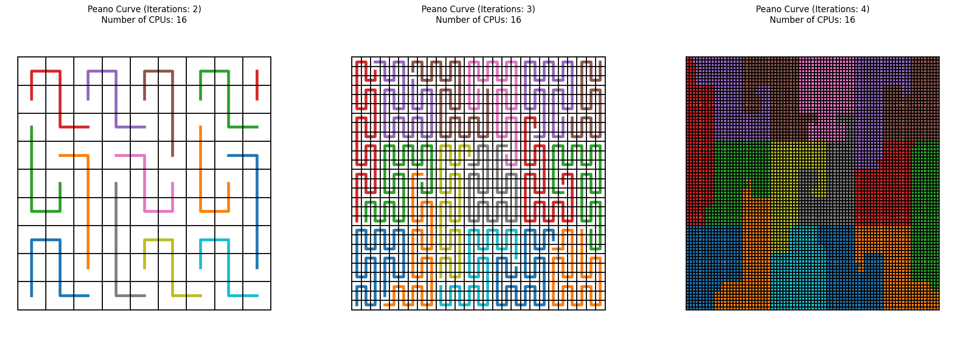
I just said that we get a pretty decent inter-processor boundary by default, but the Peano curve doesn’t seem to have an interest in doing this. Well, let’s have a look at the Hilbert curve and see how it handles the domain decomposition:
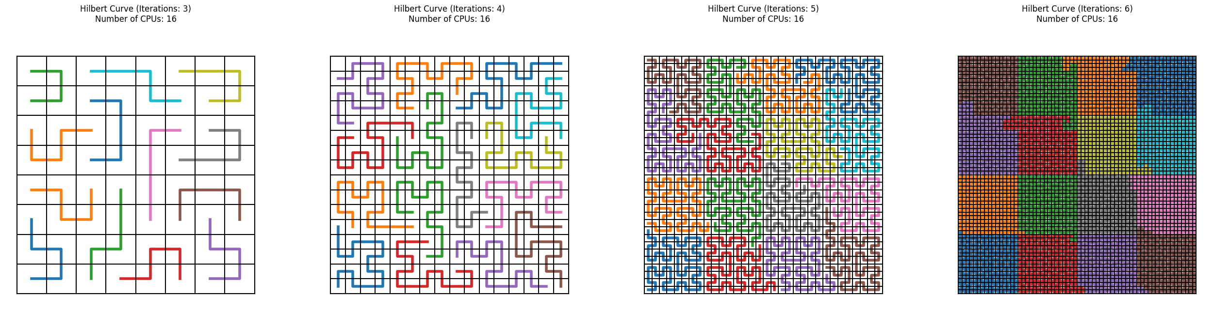
Pretty good, don’t you think? As I said, it isn’t perfect, and with a bit of tweaking, we can certainly improve things, but given that our domain decomposition essentially consists of only splitting the space-filling curve into equally long pieces, we are getting a pretty good result for not trying very hard.
OK, let’s change things up a bit. Now I want to use 9 cores, let’s see how our Peano and Hilbert curves are doing now. For the Peano curve, I am getting:
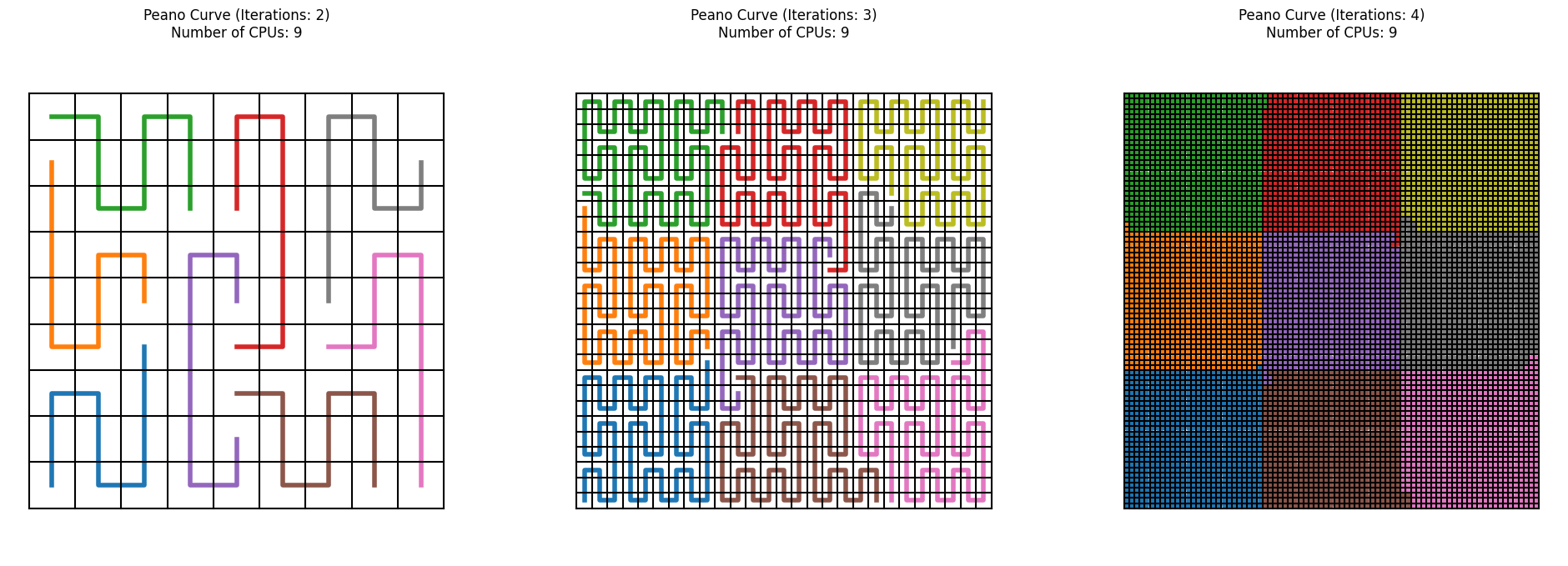
And for the Hilbert curve, I am getting:
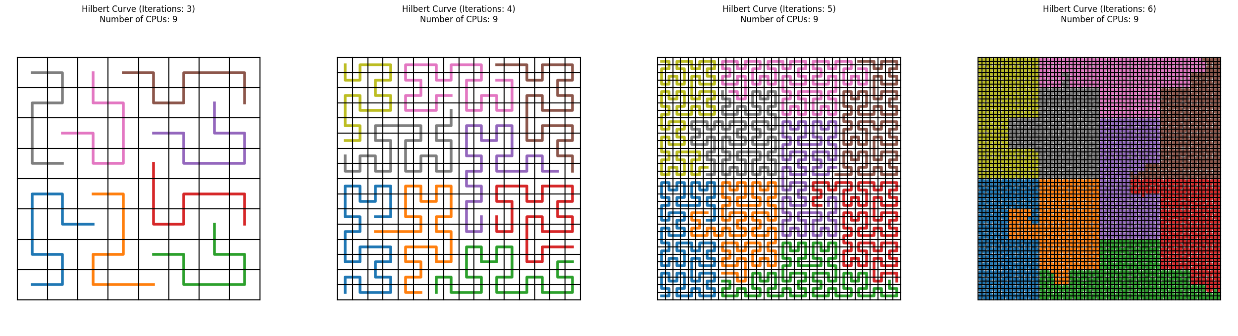
The results seem to be reversed. Can you work out why? Look at the zeroth iteration of the Hilbert and Peano curve. The Hilbert curve needs a 2 by 2 grid, while the Peano curve requires a 3 by 3 grid. In computer science, everything is binary-based, i.e. we use binary numbers and the number of cores on a CPU follows a base 2 distribution (i.e. it follows N_{cores} = 2^N where N is an integer).
We already discussed that for this reason, it is best if the number of cores follows the same base 2 distribution rule when we determine the optimal number of cores. And so, having a base 2 by 2 grid to start our space-filling curve aligns well with our needs in computer science for everything to be based on multiples of 2.
Should we ever decide to ditch our binary number basis in computer science for a ternary number basis (base-3), then Peano curves will shine, as they are already based on a 3 by 3 grid.
Thus, if we are using space-filling curves as a domain decomposition approach, Hilbert curves are the ones we want to use. I should say, though, that there are quite a few more space-filling curves out there. For example, the Sierpinski curve and Z-order curve (also known as the Morton space-filling curve) are two examples which are quite popular.
For example, when I was working with the Discontinuous Galerkin (DG) method, having several integration points per face, all of these were arranged with a Z-order curve. This was important because I was using an implementation where all elements/cell types were projected onto a unit element, and I needed to make sure that the integration points on the faces matched with their neighbours, so a consistent order was required. So, spacing-filling curves have much more subtle use cases as well.
The Sierpinski curve, on the other hand, can be used for triangular and tetrahedral meshes, extending the idea of space-filling curves to unstructured grids as well. So, before you get all excited and want to create your own space-filling curve, there isn’t much space left for more curves. It seems this space is filled already (OK, I stop now).
Another beautiful property of space-filling curves is that mesh refinement is something they handle out of the box without any problem. Take a look at the following example, where the Hilbert space-filling curve is traversing a grid with different levels of refinement:
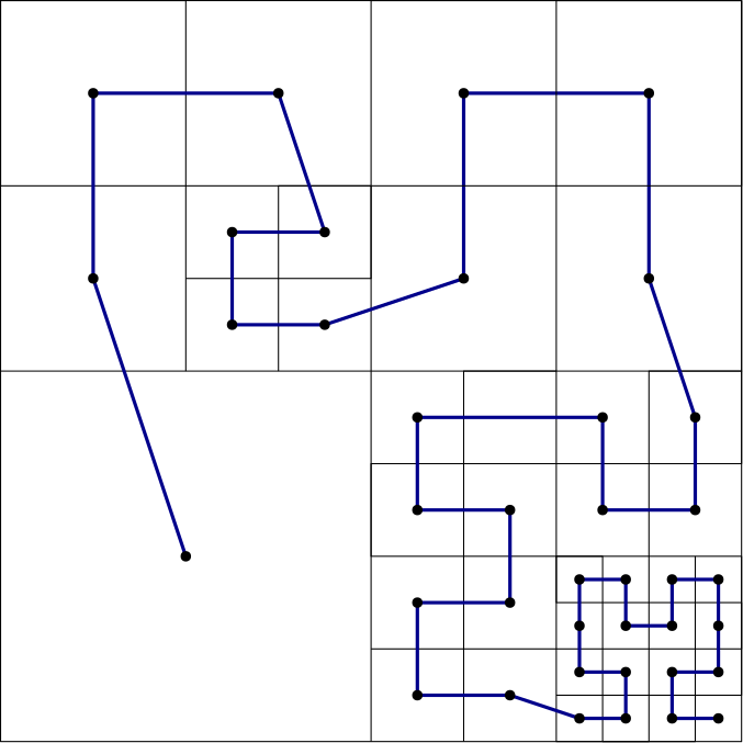
So, it seems, space-filling curves are the future in domain decomposition, right? I wish this were the case, but it is not. They work really well if all we ever want to deal with are Cartesian grids, or even Cartesian cut-cell grids with some modifications. But I’m afraid it is not that simple.
While Cartesian grids are definitely again on the rise in CFD, with almost every commercial and some open-source CFD solvers advocating the use of a Cartesian grid for the most part of the domain, Cartesian grids have one strong weakness: the number of cells required to resolve boundary layer flows becomes excessive!
For this reason, we typically build our 3D volume mesh first and then add inflation layers on top of that, which are far more economical than using Cartesian grids to resolve the boundary layer. The cells of the Cartesian mesh which overlap with the inflation layers are then removed, and both grids are then connected.
Doing this will destroy our space-filling curves, and so, if we are interested in even just moderately complex 3D turbulent flows, space-filling curves are not here to save the day (but at least now you have an idea about them and perhaps feel also slightly intrigued by them, just as much as I do).
So, if we want to come up with a general domain decomposition approach, we have to leave the wonderful world of space-filling curves behind us and start looking at graph partitioning and how this can be applied to any type of mesh.
And, if you happen to teach CFD at Imperial College, don’t worry, you can skip the next section. I don’t want to be the one telling you Santa Claus isn’t real, so keep using your hierarchical domain decomposition approach and be happy with it. Instead, here is a German proverb (I’ll even translate it for you): “The dumbest farmers have the biggest potatoes”. While me and the others talk about graph-partitioning, I’ll let you figure out what it means for you and your domain decomposition approach.
The gold standard: Graph partitioning-based domain decomposition
Let me start this section with an example that all of us should be familiar with: Group work. As a student, you will at some point likely have gone through group work during your studies, as a graduate, you will know this better under the name teamwork, and as an academic, well, you will have to organise and coordinate group work activities.
We all know that there is always a chance that people don’t get along in a group, and that can reduce the productivity of the entire group. When I started to teach at the university, the person coordinating one of the group projects I was involved with put students into groups at random, with predictable results: there were conflicts in each group, and overall, the group project suffered from it.
That person told the students that it is important to have a professional working relationship and be functional as a group, even if you don’t get along personally. The same academic was embroiled in many conflicts at work, all due to personal reasons, going as far as putting colleagues in hospital. Leading by example.
In any case, let’s look at a possible group formation. The table below shows 3 groups, where each group contains 3 students. We can assume that students are put into groups at random or in alphabetical order. It doesn’t really matter how we put them into their groups, but the important fact is that we provided the group structure, and the students were not allowed to group themselves into groups.
| Group 1 | Group 2 | Group 3 |
| Student 1 | Student 4 | Student 7 |
| Student 2 | Student 5 | Student 8 |
| Student 3 | Student 6 | Student 9 |
We can ask each student now which group members they would have preferred to stay with (for example, their friends). Let’s say we get the following answer:
- Student 1 wants to stay with Student 8 and Student 9
- Student 2 wants to stay with Student 5 and Student 7
- Student 3 wants to stay with Student 4 and Student 6
If we wanted to visualise this, we could express the table above slightly differently, in visual form. The figure below shows each student represented as a vertex (numbered 1 to 9). We then connect the vertices (students) who would like to work together. We arrange them into 3 columns, like the table above, where we have students (vertices) 1 to 3 on the left, students (vertices) 4 to 6 in the middle, and students (vertices) 7 to 9 on the right.
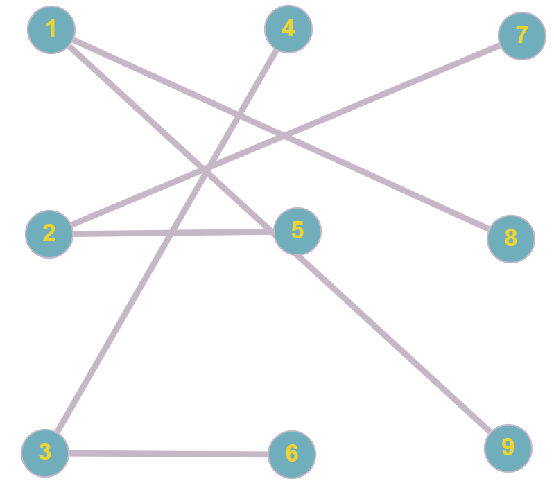
What this figure shows us is how many connections there are between groups, and this representation is known as a graph. We can now see that we have 3 connections (which are called edges in a graph) from students (vertices) in group 1 to group 3, but no connection from group 2 to group 3, for example. If we now change the group composition so that we respect the preference of students, then we end up with the following graph representation:
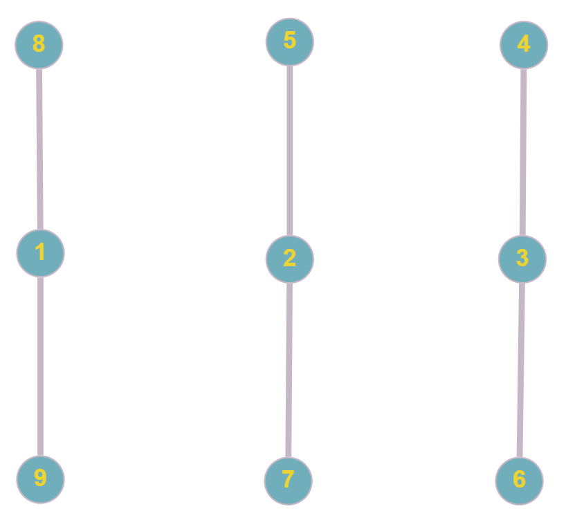
This looks much cleaner, doesn’t it? Let’s change this example to a company. We have three groups working on the same product. Some people work together (for example, the CAD and CFD engineer may work closely together), while others do not work together (for example, finance and the CAD or the CFD engineer). We have three offices in three different cities.
In each group, we can represent employees as vertices. And, if they have to work closely together (on a daily basis, for example), we can connect these vertices (employees) through an edge in our graph. So, instead of thinking of the edges in our graph as friendships, these show now the dependencies of who is working together.
Using the same two graphs we saw before, we can see that the first graph will result in a lot of communications between the three different groups in the three different cities (we assume, again, that the three different teams/groups are separated by the three different columns). If we imagine the cities to be spread around the world, we may have a situation where one employee is waiting for an answer from someone else who is currently not working because they may be several time zones ahead or behind. Not good for productivity!
If we, instead, arranged all employees as seen in the second graph so that there are no edges across teams/groups, then all communication can happen internally, and all groups could work independently.
Now imagine that instead of students or employees, the graph represents our computational mesh. Each vertex corresponds to a cell in our mesh (so, in our example above, we would have 9 cells), and each edge represents which cells (vertices) are connected, i.e. they share a face and are neighbouring cells.
If we create such a graph of our computational mesh, then we can use this graph representation for our domain decomposition. We simply divide the number of vertices in our graph by the number of processors we want to use for our parallel computation. This will give us a good load balance. But how do we group cells (vertices) together so that we have the least amount of communications across inter-processor boundaries?
Well, the edges represent neighbouring elements, and communications are always done between neighbouring elements. For example, if I am trying to solve the heat diffusion equation:
\frac{\partial T}{\partial t} = \alpha\frac{\partial^2 T}{\partial x^2},\tag{34}and I use a finite-difference approximation of the form:
T_{i}^{n+1} = T_i^n + \frac{\alpha\Delta t}{(\Delta x)^2}\left(T_{i+1}^n - 2T_i^n + T_{i-1}^n\right)\tag{35}then I can say that for cell i, the neighbouring cells are located at i+1 and at i-1. If, for example, i+1 is on a different sub-domain and solved for by a different processor, then I will need to communicate with that processor to give me T_{i+1}^n. However, I don’t care, for example, about T_{i+7}^n, because this is not my direct neighbour at location i and thus not part of my finite-difference approximation for T_i^{n+1}. Therefore, I will only need values for T from the direct neighbours of cell i.
With that knowledge in hand, we can try to cut our graph that represents the computational mesh into equal sub-domains (same number of vertices), subject to minimising the number of edges between the partitioned graph (minimising the number of neighbours between sub-domains, or, minimising the inter-processor boundary).
This is the basic idea of graph partitioning and how we can use it for the task of domain decomposition. If we want to do that, though, we first need to know how we can create the graph in the first place.
I mentioned above that we create a graph by first drawing as many vertices as there are cells in the mesh, and then connecting those vertices with an edge that are next to each other in the mesh (neighbouring cells). Take, for example, the following structured mesh:

On the left, we see the 3 by 3 structured mesh, and each cell has its own cell ID. On the right, we see a matrix with crosses. A cross represents a neighbouring cell pair. So, for example, cell 1 and cell 2 are neighbours, and so in row 1, column 2, we have a cross. We also place a cross in row 2 and column 1, because the connection goes both ways (i.e. cell 2 is a neighbour of cell 1 (first row), but cell 1 is also a neighbour of cell 2 (second row)).
So, we go through each row in the matrix, where the row ID corresponds to the cell ID, and we put a cross into each column, where the column ID corresponds to the cell IDs of neighbouring cells. If two cells are not neighbours, then there will be no cross. This representation is fairly common and represents a matrix structure.
Later, when we discretise our system of equation and we solve it, for example, with an implicit solver (i.e. we are solving the system \mathbf{Ax}=\mathbf{b}), then we would get the same matrix structure as seen above for \mathbf{A}, except that instead of crosses, we get numerical values. Cells with no crosses will have a zero. If you want to have some additional explanation with examples of how to construct this type of matrix, I have a dedicated article on how to assemble these types of matrices.
We can then use this matrix to identify neighbouring cells. For any given cell ID, we go into that row and check which columns have a cross. For example, cell 5 (row 5) has cells 2, 4, 5, 6, and 8 as neighbouring cells. Yes, we count 5 here as well, which is perhaps somewhat confusing, but only if we think of edges as neighbours. Technically speaking, the edges represent the cells that are required to compute an updated solution.
For example, to compute T_i^{n+1}, we don’t just need its neighbouring values, i.e. T_{\pm 1}^n, but also the value at i itself, i.e. T_i^n. Thus, we say that cells depend on themselves, and that is why cell 5 has cell 5 listed as its neighbour.
We can now draw out the graph again, by placing all vertices (9 in total) and then connecting them so that each neighbouring cell is connected through an edge to its neighbour. We obtain the following graph:
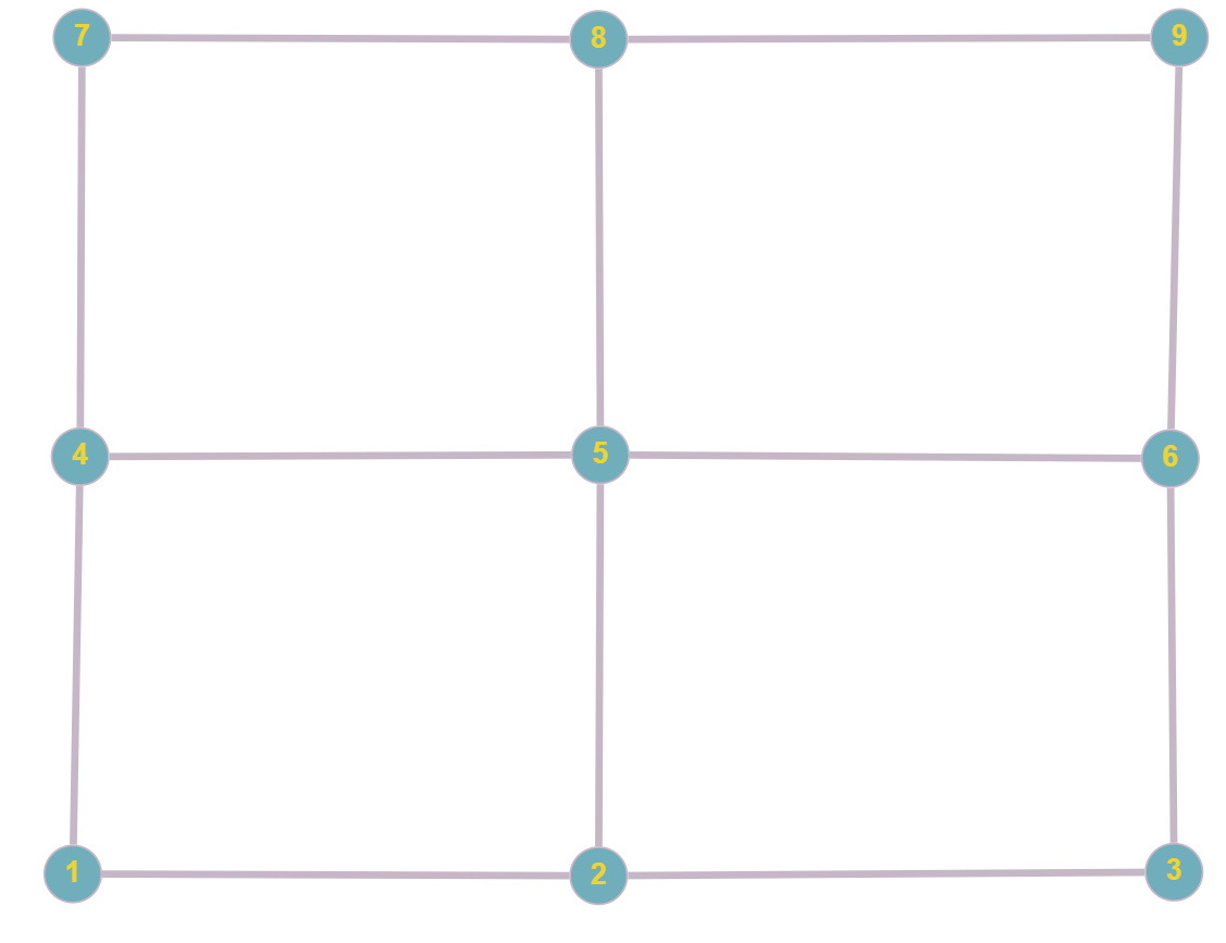
This looks pretty much like our structured grid, doesn’t it? However, we could have also drawn the graph in a completely different order, as seen below:
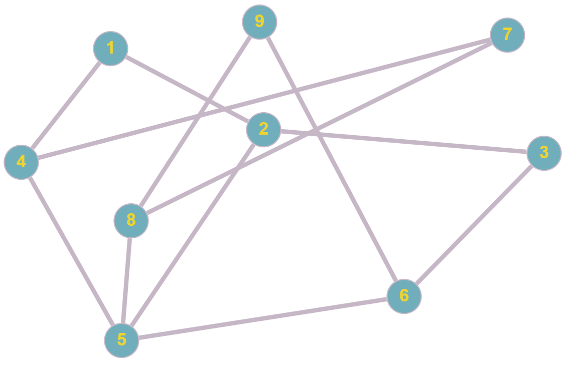
The graphs in the previous two figures are identical. You can verify that by looking at which vertices are connected, and you will see that they have exactly the same connections. Thus, a graph can be drawn arbitrarily, and some representation may help better see the inherent structure the graph represents, for example, a structured grid.
Now, imagine I asked you to partition your graph into three equally sized graphs, while minimising the number of edges between graphs. Go back to the previous graph, and you can see that two cuts, either horizontally or vertically, will result in 3 partitioned graphs. This is shown in the following for the first two figures:
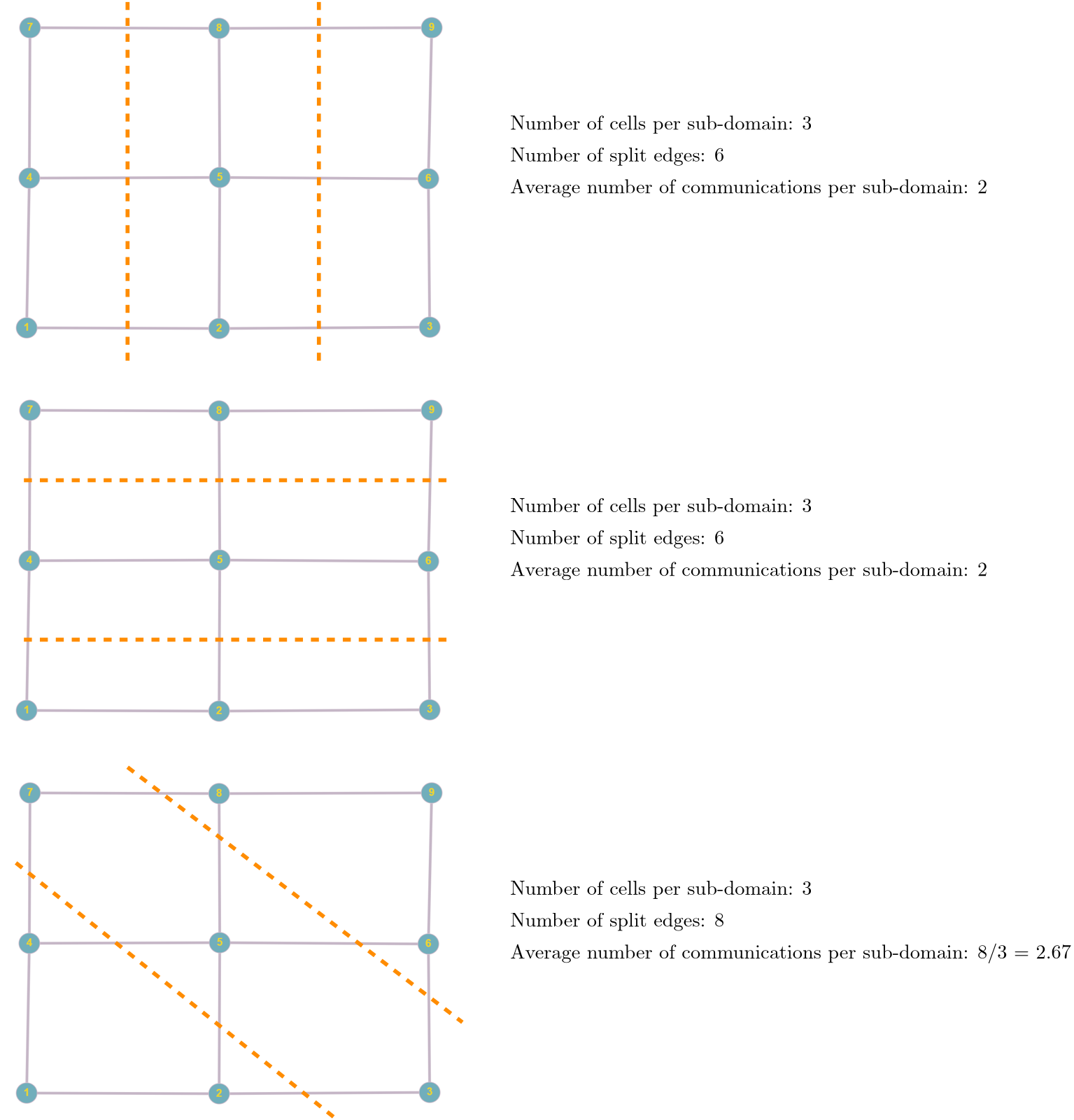
In the last example, I have cut the graph diagonally, which results in a total of 8 edges being cut (which means we have a total of 8 communications, or an average of 2.67 communications per sub-domain). Compare that to the vertical and horizontal cut, which results in only 6 total communications, or 2 per sub-domain, on average.
The nice thing about graph partitioning is that it only requires information about neighbouring cells, nothing else, and so this can be easily extended to unstructured grids as well. Take the following unstructured grid, for example, where I have shown the same matrix as in the previous example, where we can read neighbouring cell IDs directly for each cell by going to its corresponding row:

We can construct the graph from this matrix as:
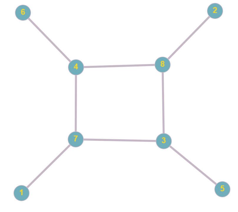
We can now consider, again, how we would have to cut this domain so that we have the same number of vertices per sub-domain and the least number of edges that connect vertices between sub-domains.
The only thing we need now is some form of algorithm that can do that for us. We are in luck, people have thought about this problem a long time ago, and we simply have to pick whichever algorithm we prefer the most. A good algorithm to get started is the Kernighan-Lin algorithm, or K-L algorithm in short. It is rather slow, but with a few adjustments, it can be made performant again. So, let’s review this algorithm.
The K-L algorithm takes an existing graph and will produce two balanced, disjoint (not-connected) graphs, where communications (edges between disjoint graphs) are minimised. We have to provide two disjoint graphs as an input, but we do not have to care whether they are already balanced (i.e. the edges between graphs are minimised). Some of you may have realised one limitation of the algorithm: we can only partition a graph into two graphs, not an arbitrary number of sub-graphs (equivalent to sub-domains in our case).
This is yet again another reason why we should partition our mesh with 2^N sub-domains, with N being an integer, because our algorithms work best for these cases. Having said that, modifications have been introduced to allow for an arbitrary number of sub-domains (disjoint graphs), though these are corrections and thus may not necessarily yield the most optimal graph. We are standing a much better chance if we stick to 2^N partitions.
Let’s go through the algorithm step by step with an example graph, which is shown in the following figure:
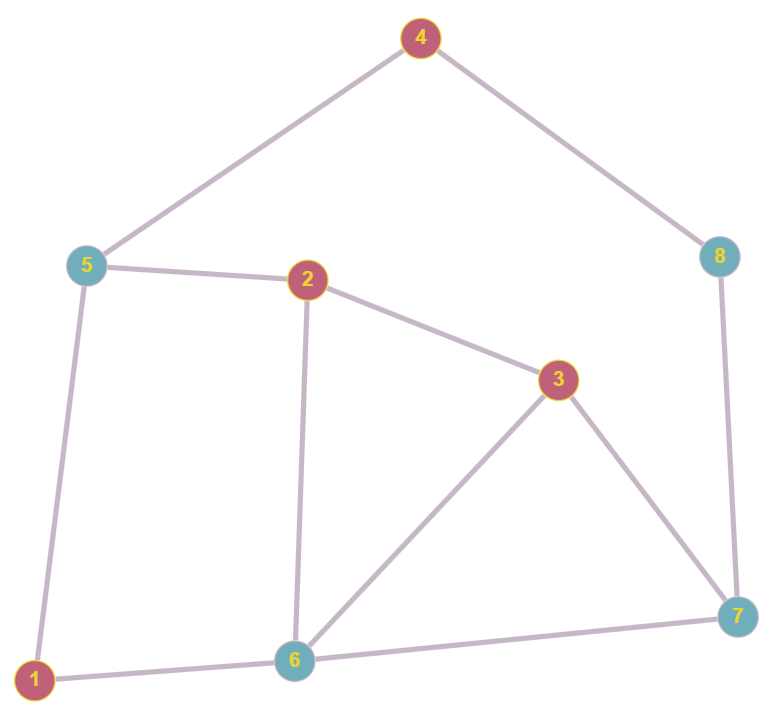
Here, I have already coloured the vertices based on an initial distribution I have come up with. Well, we can see that it is probably not optimal, but that is good, so we see how the K-L algorithm works and improves our partition. I have grouped the 8 vertices into two initial partitions as:
- Graph A: Vertices {1,\,2,\,3,\,4}
- Graph B: Vertices {5,\,6,\,7,\,8}
So you see, coming up with an initially partitioned graph isn’t really a problem; we just assigned the first half of the vertices to subset A and the second half of the vertices to subset B.
Now, the K-L determines the cost for each vertex, which is given as:
D(v) = E(v) - I(v) \tag{36}Here, v is any of the vertices, i.e. vertex 1 to 8 in our example, and E(v) and I(v) are the external and internal costs, respectively.
The internal cost is the number of edges for vertex v that connect to other vertices in the same graph. That is, if v is part of A, then any edge to vertices 1, 2, 3, or 4 would be counted as internal edges. If v was part of B, then any edge connecting it to vertex 5, 6, 7 or 8 would be an internal edge. Thus, I(v) is the number of edges that exist in the same graph.
The external cost, on the other hand, is the number of edges that connect v with vertices in the other graph. Thus, if v is in A, then any edge connecting it to 5, 6, 7, or 8 would be counted as an external cost. Similarly, if v is in B, then any edge connecting it to vertices 1, 2, 3, or 4 would be an external edge as well.
This sounds all wonderfully abstract, so let’s see that with a concrete example. Take vertex 5, which is in B. It has a total of 3 edges, and all of them point to vertices in A, so E(5) = 3. There are no edges connecting it to vertices in B, and so I(5) = 0. Thus, we can compute the cost as D(5) = E(5) - I(5) = 3 - 0 = 3.
We do this calculation now for each vertex, which results in the following table:
| Vertex | E(v) | I(v) | D(v) |
| 1 | 2 | 0 | 2 |
| 2 | 2 | 1 | 1 |
| 3 | 2 | 1 | 1 |
| 4 | 2 | 0 | 2 |
| 5 | 3 | 0 | 3 |
| 6 | 3 | 1 | 2 |
| 7 | 1 | 2 | -1 |
| 8 | 1 | 1 | 0 |
Let’s look at these values and the graph that we saw before. If we get a high value for D(v), then we have lots of connections between A and B (or, rather, we have more external than internal edges). So, it stands to reason that we want to look at those vertices that have a high D(v) value and see what we can do about them. The highest value is obtained for vertex 5, with D(5) = 3 as we have calculated before. However, if 5 had been part of A, then D(5)= -3, because now all edges would be internal edges.
Thus, high values of D(v) indicate potential of swapping in order to reduce the number of external edges (communications), while low values indicate that we want to keep them in the subset they are already in.
If we stick with vertex 5, then we have established that swapping it with a point in A would be beneficial. But which one? We need another equation that will determine which pair of vertices will provide the most optimal swap. For this simple example, we can likely work that out ourselves, but if our graph has, say, 76,584 vertices, it’ll be slightly more complicated, so let us instead think about how we can achieve that.
We have established that vertex 5 in subset B should swap with one of the vertices in subset A. So, our goal is to find a vertex in A that has a high value of D(v) as well. This high value would indicate that a swap would be beneficial for that vertex as well. In our example, we see that both vertex 1 and 4 have a value of D(1) = 2 and D(4) = 2. Thus, a swap between vertices 1 and 5 or 4 and 5 would be ideal.
Mathematically, we could say that we want to maximise D(a) + D(b), where a are vertices in A (i.e. 1, 2, 3, and 4) and b are vertices in B (i.e. 5, 6, 7, and 8). Let’s look at vertex pair 1 and 5. When we counted the external edges, we counted the connection from 1 to 5 when we computed the external cost for vertex 1, and we counted the connection between 5 to 1 when we computed the external cost for vertex 5, respectively. When we swap 1 and 5, this external edge will still exist.
Therefore, if we swap vertices 1 and 5, we will still retain this external edge, and it will appear twice, i.e. going from vertex 1 to 5 and going from vertex 5 to 1.
Thus, if we say that we want to find the highest value of D(a) + D(b), we need to subtract a value of 2 from it if, and only if, vertices a and b share an edge between them, to account for the fact that after the swap, this external edge still exists.
Putting all of this together, we can compute the so-called Gain of vertex pair a and b as:
Gain(a,b) = D(a) + D(b) - 2c_{a,b}
\tag{37}
Here, D(a) and D(b) are defined as before, and the additional term -2c_{a,b} accounts now for a potential external edge between vertex a and b. The value of c_{a,b} is 1 if an edge between a and b exists, otherwise it is 0. In our example, we have c_{a,b}=c_{1,5}=1, because both 1 and 5 are connected through an edge.
Therefore, the computed gain between a and b is reduced. Our goal is to find the maximum value of Gain(a,b), so that we identify the best pair of vertices to swap. Thus, we have to compute the gain for each vertex pair. Remember, since a is in A and b is in B, we only have to compute the gain of a with elements in B, and vice versa. The following table shows this computation:
| Vertex pairs | D(a) | D(b) | c_{a,b} | Gain(a,b) |
| {1,5} | 2 | 3 | 1 | 3 |
| {1,6} | 2 | 2 | 1 | 2 |
| {1,7} | 2 | -1 | 0 | 1 |
| {1,8} | 2 | 0 | 0 | 2 |
| {2,5} | 1 | 3 | 1 | 2 |
| {2,6} | 1 | 2 | 1 | 1 |
| {2,7} | 1 | -1 | 0 | 0 |
| {2,8} | 1 | 0 | 0 | 1 |
| {3,5} | 1 | 3 | 0 | 4 |
| {3,6} | 1 | 2 | 1 | 1 |
| {3,7} | 1 | -1 | 1 | -2 |
| {3,8} | 1 | 0 | 0 | 1 |
| {4,5} | 2 | 3 | 1 | 3 |
| {4,6} | 2 | 2 | 0 | 4 |
| {4,7} | 2 | -1 | 0 | 1 |
| {4,8} | 2 | 0 | 1 | 0 |
We now pick the value with the highest gain, which is either vertex pair {3,5} or {4,6}. If we have two or more equally good choices, we pick one at random. So let’s pick the first pair and swap vertex 3 with vertex 5. Our new updated subsets (sub-graphs) become:
- Graph A: Vertices {1,\,2,\,\mathbf{5},\,4}
- Graph B: Vertices {\mathbf{3},\,6,\,7,\,8}
The corresponding visual representation is:
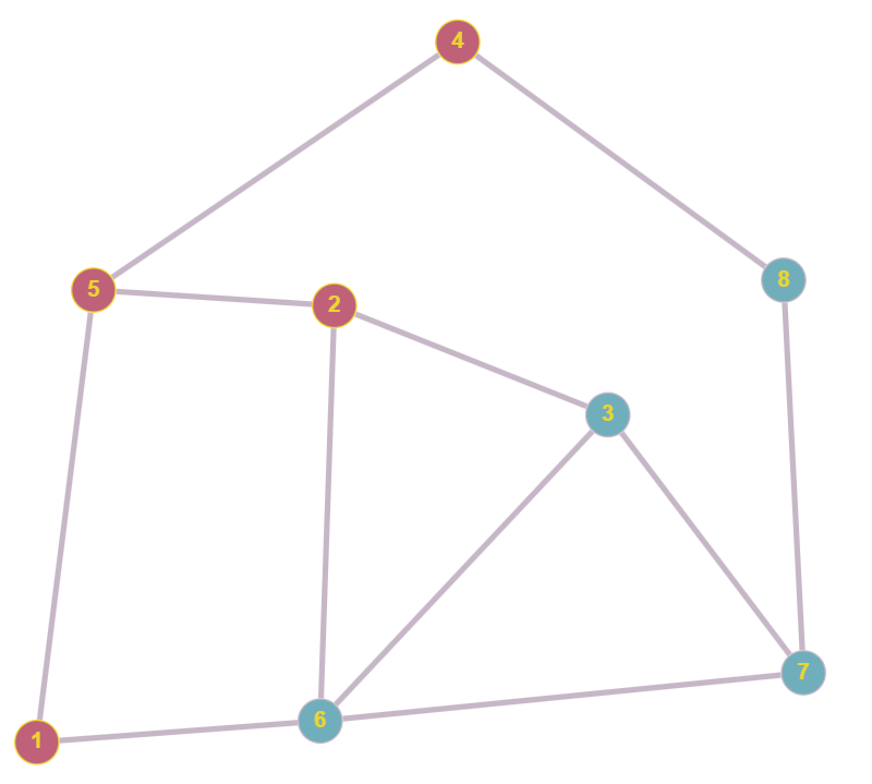
We now repeat this algorithm, but we lock down vertices 3 and 5. If we find in the next step that the highest gain involves either vertex 3 or 5, we cannot use it. If we did, we would just undo the work of the previous step, and we would never finish.
In this example, we have already found one of the many optimal solutions. Vertex 2 has two external edges, and so we may be tempted to swap it with vertex 8. This would reduce the external edges for vertex 2 to a single external edge, but vertex 5 would also gain a new external edge, so we would not gain a lower number of external edges (and thus, we would still have the same number of communications).
So, we have found our optimised graph from an initial partition of two subsets (sub-graphs, sub-domains, etc.). Now, if I left it at this, my inbox will be filled with hate speech of Imperial fanboys and fangirls, and probably rightfully so. Why? Let’s look at the computational cost of the Kernighan-Lin algorithm.
When we compute the gain in Eq.(37), we have to evaluate each vertex pair a and b. Let’s say we have 1 million cells in our mesh, and we want to split this into 2 sub-domains using the Kernighan-Lin algorithm. Then, we compute the gain for the first vertex (first cell in the mesh) against all 999,999 other vertices (cells) in our graph. Then, we go to the second cell, and we compute its gain with all 999,999 other vertices in the graph.
Thus, for each vertex, we compute the gain with itself and 999,999 other vertices, and we have to do this a total of 1 million times for all cells involved in our mesh. This is pretty expensive (and this is an understatement!). But we are not done yet! All that we have done is swap a single vertex pair based on the best gain value. Once we have done that, we lock these two vertices and then repeat the process until there is no further gain. This expense is ludicrous!
When we want to define the time it takes for an algorithm to run, we use the big O notation. It tells us the expense of an algorithm in terms of the number of elements n. In our example, n is the number of cells in our mesh, or vertices in the graph. We don’t necessarily count every calculation, but we want to get an estimate for the algorithm’s cost as an order of magnitude estimation.
In our example, we saw that we have to compute the gain for each cell, and we do that with all cells except itself. We can express this cost as n\cdot (n-1). However, this is just a single evaluation, and we need to do that for each cell. Thus, we could write the computational cost as (n\cdot(n-1))^2. Now, as an order of magnitude, we can say that this is approximately equal to (n\cdot(n-1))^2\approx n^2, and this is how we compute the cost for the first pass.
Next, we have to repeat this process for as many elements as we have in n. However, since we already found one vertex pair to swap in the previous step, we don’t need to consider it in the next step. Thus, each subsequent step in the Kernighan-Lin algorithm reduces in computational cost, which is expressed as \log(n). Therefore, the overall cost, using the big O notation, is: \mathcal{O}(n^2 \log(n)). This is just ridiculous. Let me show you why.
Let’s compute a few of these values. The following table shows, in the first column, the number of cells we could have in our mesh. These would then also represent the number of vertices in our graph that we want to partition. The second column computes the value for n^2 \log(n). The third column simply divides the second column by 3\cdot 10^9, i.e. the number of operations a CPU can perform per second, typically. This assumes that all computation in the Kernighan-Lin algorithm can be performed in one clock cycle (we can’t), but as an order of magnitude computation, this will do. In reality, the cost will be slightly higher here.
Thus, the third column gives us an idea of how long it would take to partition our graph, and the fourth column just provides the same value but now expressed in days, rather than seconds, to make the numbers easier to interpret.
| Number of cells | \mathcal{O}(n^2 \log(n)) | Cost in seconds | Cost in days |
| 1 | 0 | 0 | 0 |
| 10 | 1\cdot 10^{2} | 3\cdot 10^{-8} | 4\cdot 10^{-13} |
| 100 | 2\cdot 10^{4} | 7\cdot 10^{-6} | 8\cdot 10^{-11} |
| 1,000 | 3\cdot 10^{6} | 1\cdot 10^{-3} | 1\cdot 10^{-8} |
| 10,000 | 4\cdot 10^{8} | 1\cdot 10^{-1} | 2\cdot 10^{-6} |
| 100,000 | 5\cdot 10^{10} | 2\cdot 10^{1} | 2\cdot 10^{-4} |
| 1,000,000 | 6\cdot 10^{12} | 2\cdot 10^{3} | 2\cdot 10^{-2} |
| 10,000,000 | 7\cdot 10^{14} | 2\cdot 10^{5} | 3 |
| 100,000,000 | 8\cdot 10^{16} | 3\cdot 10^{7} | 3\cdot 10^{2} |
We can see that if we have 10 million cells in our mesh, we can expect the Kernighan-Lin algorithm to take 3 days to find us an optimal partition. 10 million cells isn’t a lot in CFD terms. If I give an assignment to students, I typically expect them to run simulations with roughly 10 million cells. In their research project, they may go up to 50 million cells, and simulations of my PhD students (and my own simulations) can easily reach 100 million cells.
But that is not the limit; both industry and academia are running simulations with billions of cells, and this is becoming the norm; it is no longer the exception. And so, if I run my simulation with 100 million cells, I don’t want to wait 300 days before my Kernighan-Lin algorithm has found an ideal distribution to reduce communication cost; any sub-optimal domain decomposition (yes, even the Imperial College approach) would have been better, and I would have received my results earlier.
And, keep in mind, that after the Kernighan-Lin algorithm is done, we have only divided the domain into 2 sub-graphs. We need to now repeat the same process for each sub-graph until we have reached the desired number of sub-graphs. No, thank you!
Thus, while conceptually easy to understand, we use the Kernighan-Lin algorithm to explain how graph-partitioning works, but not in CFD codes. However, many other algorithms have been developed that use this algorithm as their baseline, and they simply improve on the bottleneck.
For example, the Fiduccia–Mattheyses algorithm is essentially an extension of the Kernighan-Lin algorithm, but it is so efficient that it reduces the computational cost from \mathcal{O}(n^2 \log(n)) to \mathcal{O}(E), where E is the number of edges. Thus, we have reduced the time complexity from something exponential to something linear, meaning our graph partitioning scales now linearly with our mesh size.
How does the Fiduccia–Mattheyses algorithm achieve this? Well, in a nutshell, the first problem of the Kernighan-Lin algorithm is that it has to evaluate vertex pairs, which gives it an n^2 computational cost. In the Fiduccia–Mattheyses algorithm, we loop over vertices and swap them as we compute their gain. We keep a so-called bucket list that shows us the current highest gain, and we can think of it as a high-score system. Thus, if the current gain is not beating the high score, it may not be optimal to swap.
This reduces the complexity to having to loop over all edges E, and since we swap vertices as we visit them, we typically only have to do a few passes, at most, retaining the linear time complexity of \mathcal{O}(E).
While this is a huge improvement, we don’t stop there. The next thing we introduce are multilevel graph partitioning algorithm. The idea behind these algorithms is to reduce the original graph to a smaller graph. Take the following graph as an example:
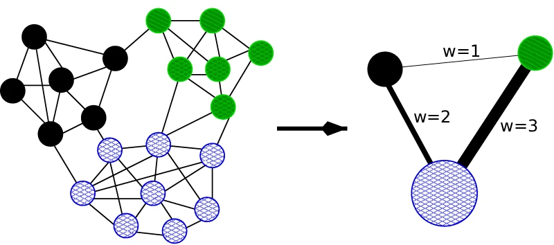
On the left, we have our original graph. We see that there are only a few edges between each subset, where each vertex in a different subset is given a different colour and pattern. What we do now is to coarsen the graph to only a few vertices, as we see on the right. We don’t care about all of the individual vertices in one subset, as these will anyway stay within that subset, but what we do care about is the number of external edges.
When we coarsen our graph, we will lose these external edges, and so what we do is to introduce a weight w for each external edge. The weight represents the number of external edges that are represented by a single edge. We can see in the example below that the external edges on the right account for 1, 2, and 3 external edges that we see on the left, i.e. the original graph.
Now, when we calculate the gain between vertex pairs, instead of just counting external edges, we need to multiply each external edge by its weight to get the true gain, as each external edge potentially represents a number of external edges. After we have done the partitioning on the coarsened graph, we have to apply that again to the original graph.
We may wish to introduce several levels (i.e. different coarse graphs) and perform this step on each of these subgraphs, which improves the graph partitioning for each level and thus for the original graph, while keeping the computational cost low.
In spirit, this idea is very similar to how multigrids work in CFD applications, where we compute the solution first on a coarse grid with just a few hundred cells. This result will be inaccurate, but if we interpolate that now into a finer grid, we can compute a new solution that is more accurate, and since we have a better initial guess for the solution from the coarse grid, it won’t take as long to compute a new solution, and the computational cost is overall reduced.
If we now combine the Fiduccia–Mattheyses algorithm, for example, with multilevel graph partitioning algorithms, we can easily partition a mesh with several million cells into as many sub-domains as we want in a matter of seconds. Now that is what I call efficiency.
Parallelisation frameworks
Now that we have a good understanding of how parallel computations are enabled by hardware, how we can benchmark and find bottlenecks in parallel code, as well as how to efficiently distribute a computational mesh across several processors (sub-domains), it is time to look at some of the parallelisation frameworks that enable us to do computations in parallel.
In this section, we will first look at the differences between shared and distributed memory models, and what that means to our parallelisation effort. Next, we will write a very simple unsteady, 1D heat-diffusion code that we then parallelise using both CPUs and GPUs.
Shared and distributed memory approaches
Whenever we pick a parallelisation strategy, the first question we have to ask ourselves is: “Do we want to use a shared or distributed memory approach”? This must be the first question we ask, because everything else derives from it (i.e. the domain decomposition approach, the parallelisation framework, the types of application we can and can’t solve, and the list goes on).
Let’s look at the following schematic to see what their differences are:
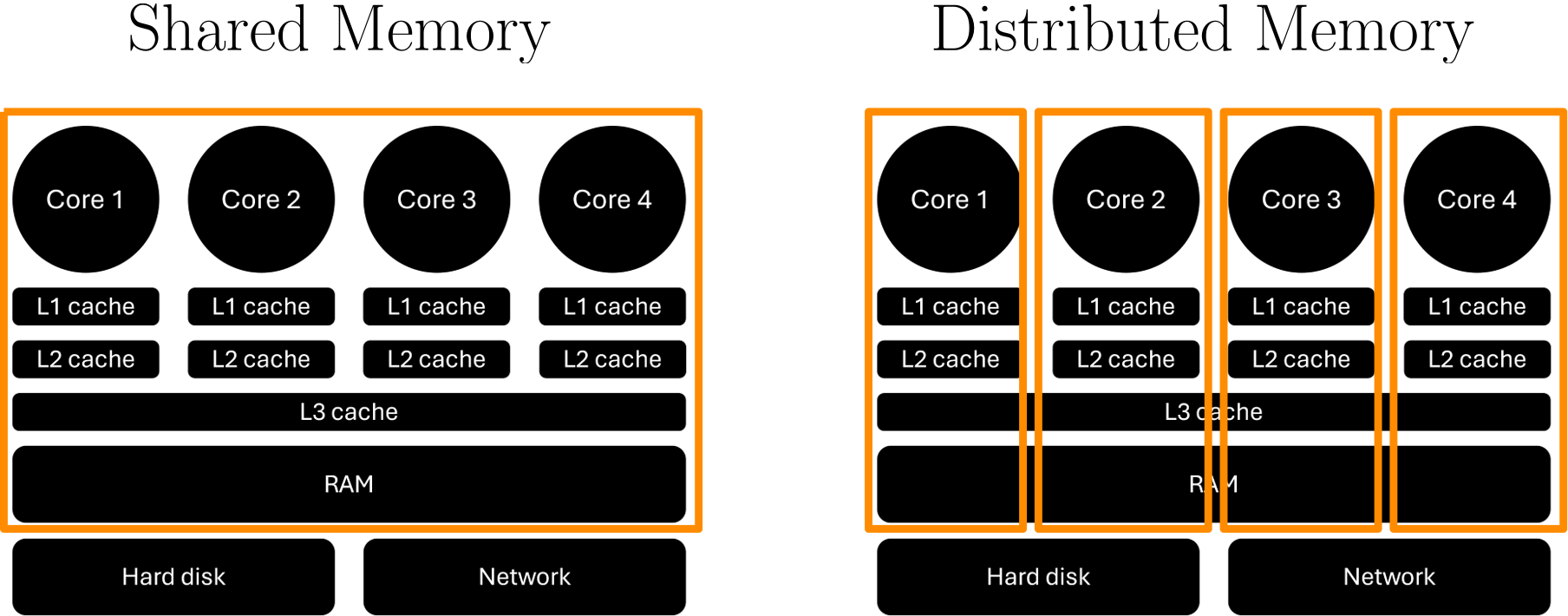
What I have shown here is an orange box around various parts of the CPU. On the left, the orange box encloses all processors, or cores, including all local and shared caches, as well as the RAM. What this means is that each processor, or core, has access to all memory. Theoretically, it can see what is in the caches of other processors, but as we have discussed above, these caches only help us to bring data to the processor so that access times are accelerated. So, there is no need to access these access accelerators.
Instead, what we mean by shared memory is that each processor has access to the entire RAM and can see what every other processor can see in memory as well, and each processor can access the same memory that any other processor can access as well.
Distributed memory, on the other hand, says that each processor is separated from all of the other processors and gets its own private space in RAM. Thus, each processor will only be able to see their own private memory space in RAM, but not that of others. If one processor requires data from another processor’s private memory space, it will need to request that, and the other processor needs to send that data.
Think of a simple analogy: If we go to a park, anyone can walk on the grass anywhere without any restrictions. We can access any part of the park by going there. This is like shared memory. Then, we redevelop that part and build houses, and each house gets its own private garden, which is fenced off. We can no longer go everywhere in the park (without trespassing, I suppose). This is our distributed memory model.
If you play fetch with your dog in your garden and the ball lands in your neighbour’s garden, you will have to request permission to enter their garden (or ask them to get it for you). This is the same as how a processor has to request data from another processor in the distributed memory model.
Earlier, I spent some time preaching that sending and receiving messages is slow, and so we want to avoid communication as much as we can. Now I am saying that shared memory does not have any communications (well, at least not in the sense that memory needs to be requested from other processors, but there are still communications, just substantially fewer). So shared memory is the clear winner here, right? Well, any serious CFD solver that is parallelised uses a distributed memory approach.
The problem with shared memory is that you have access to your RAM, and all processors can use it. This is great if you have a problem that is, say, just about big enough to be solved on 4 cores, and your CPU has 4 cores or more. But, once you start to have bigger and bigger simulations you want to solve, you will need more and more cores. However, with shared memory, the maximum number of cores you can request is the number of cores that have access to your RAM.
On a desktop PC, well, that is your CPU. You cannot put a second PC next to it and then split the work across both PCs, as you would now physically split the RAM. Your shared memory model needs to see all RAM in order to work, and it does not work if it is physically separated across two PCs. It is the same as playing fetch with your dog, except you and your dog are both in different parks.
If we want to use more than one CPU and its RAM, we need a distributed memory approach. Think back to the beginning of this article, when we talked about the hardware that goes into an HPC cluster. It is packed with compute nodes, all having their own socket with cores and physically separated RAM. If you want to be able to make use of a supercomputer by using a large number of compute nodes, you need to be able to request data not just within the same CPU/socket, but from CPUs/sockets that are outside your compute node.
This brings us to the following selection criterion:
- Shared memory: We use shared memory if we expect our problem size to always fit within a single compute node with shared RAM. On a cluster, we may get as many as 128 cores; on a desktop PC or laptop, we would typically get something between 4 and 32 cores, depending on our CPU. Earlier, we said that 100,000 cells per core is a good rule of thumb for efficient parallelisation, so with 128 cores, we can compute CFD problems with 12.8 million cells efficiently.
- Distributed memory: If we expect our problem size to not fit into a single compute node, or our desktop PC/laptop, then we need a distributed memory approach. If we ever plan to run a case with more than 12.8 million cells, then we likely need a distributed approach. General-purpose CFD solvers do not want to make any assumptions here and assume that you do, indeed, want to use more than a single compute node. For that reason, you will find a distributed memory model common to all major CFD codes.
While this selection criterion seems very binary, i.e. it is either one or the other, in reality, mixed approaches are more and more common, known either as Partitioned Global Address Space (PGAS) languages, or MPI-X. We will talk about MPI, the Message Passing Interface, in this section and see that this is the mother of all distributed memory approaches. The X in MPI-X can be any shared memory approach, and so we mix MPI (distributed memory) with some shared memory approach.
While the code does not get substantially more complicated, executing the code does not come without its challenges, and it does require dedicated hardware. You can’t run PGAS or MPI-X codes on just your desktop PC or laptop, unless you decide to build your own cluster at home. You need some form of physically separated hardware in order for this approach to really work its magic, meaning you need to have access to some form of compute cluster.
Before we start writing our code to parallelise, I want to quickly introduce two common problems that you will come across in parallelised code that are sometimes difficult to spot, and so they will make your life a lot more difficult trying to track down bugs. These bugs only exist in the parallel code and not in the non-parallel (sequential) code.
Race conditions
When I went to high school, a popular summer activity was to meet in the park to have a BBQ. Believe it or not, we were not the only ones thinking of meeting in the park for a BBQ, and despite its size, spanning several football/soccer pitches, finding an empty spot where you would not sit shoulder to shoulder with other groups was difficult. So, you had to be early to reserve your seat.
But then again, I grew up in Germany, and if there is one thing Germans are good at, it is arriving early to reserve your seat, which many tourists in hotels will have found out the hard way. And, in case you have never had the pleasure to observe the Germans in the wild, here you go, the sun-lounger Olympics in Rio:
What an absolute car crash. Anyhow. If I wanted to meet with my friends at a specific location, we had no idea if that particular spot would already be occupied or not. If we all agreed to meet at that point, only to find out that it was already occupied when we arrived, we had no way of finding each other (mobile phones were not common yet).
This is a race condition, because there is a race to a particular location, and whoever comes first will get the spot and can do their BBQ there; everyone else can go back home (or, well, go somewhere else). But perhaps the next day, when we decide to meet at exactly the same place, we may end up being the first to arrive, and so we get our spot. There is no way of knowing in advance who will arrive first, and so, sometimes we get lucky, and we get our spot to do a BBQ, and sometimes we don’t.
Now, let’s translate that to parallel computing. A race condition is defined as two or more processors trying to access a particular memory location, potentially overwriting the value. So, you may have processors 1 and 2 trying to access memory location X. Both processors 1 and 2 expect the value stored at X to be, say, 10. Then, processor 1 gets there first and updates the value. Now, processor 2 gets there and instead of getting the value 10, it may get the value 20, which it does not expect, and so its computations will be wrong.
If, however, processor 2 got their first, which only wanted to read the value but not update it, it could do that, get the value for X, which should still be 10 if it got their first, and then afterwards, processor 1 could access the value and overwrite it. Depending on which processor comes first, we may get a different outcome, and this is, as already mentioned, a race condition.
Don’t worry, once you start programming in parallel, you will produce many race conditions; you can’t avoid them. If you are vibe coding, then expect lots of race conditions that ChatGPT can’t save you from; LLMs are especially weak when it comes to parallelising code.
What is important is that you recognise when a race condition occurs so that you can check your memory access in your code. If you run your code on a single core and everything works fine, but results either sometimes work or you get wrong results with your parallel code, then you may have a race condition. At this point, you want to check how memory is being accessed or sent and received.
Deadlocks
Deadlocks are another common pitfall. Imagine you work in a group with others at work, and there is one particular step you have to do before you can start working on your project. For example, you may be tasked with simulating the flow over a particular geometry, meaning the first step in this process is to obtain the geometry. You task the new guy at work to obtain the geometry, and until you get your hands on the geometry, you cannot do anything productive.
It turns out that the new guy was in reality an intern, who had their first day at the company. On the same day, the intern was caught embezzling company property, and so the intern was fired on the spot. No one told you and your group, and so you are still waiting for the intern to come back with the geometry, which will never happen. This is a deadlock.
In the world of computing, a deadlock happens when one processor gets stuck in one task, typically in a loop that never finishes, i.e. we have an infinite loop. So, now one processor is trapped inside an infinite loop while all the other processors eventually come to a standstill because they need to get some data from that processor. But, because the processor is stuck in the loop, it cannot work on any data requests, just like all of your angry emails to the intern go unanswered, as the intern has lost access to their emails.
A deadlock is easy to spot in that your code eventually stops and does not advance through the program anymore. Using caveman debugging principles, we can place a few print statements here and there in our code to figure out the exact location that produces the deadlock (i.e. we look at the lines of code between the last print statement that was executed and the next print statement that wasn’t).
Between these two print statements, something went wrong, and we can insert more and more print statements to narrow down the part of the code where the deadlock is coming from. It does not always have to be an infinite loop; there are other ways of producing a deadlock, so we don’t necessarily always just look for loops.
For example, if every processor is sending data and waiting for a response from the processor it is sending data to, before going to the next step (which is receiving the data), no processor is actually in receiving mode, and so all processors will be stuck at the sending stage. This is a common deadlock new programmers will make in parallel computing, and we will look at this particular issue later in greater detail when dealing with MPI (where it most commonly occurs).
A sequential example code
All source code that is discussed in the following sections can be downloaded using the link provided at the beginning of the article
Ok, we need to establish a baseline, and so we will develop a simple CFD solver that will solve the heat diffusion equation as:
\frac{\partial T}{\partial t} = \alpha\frac{\partial^2 T}{\partial x^2}
\tag{38}
I will just use a simple finite difference approximation here, with an explicit time integration, as this will make the discretisation very straightforward. Let’s discretise each term together. For the time derivative, we use a first-order approximation in time:
\frac{\partial T}{\partial t} \approx \frac{T_i^{n+1} - T_i^n}{\Delta t}
\tag{39}
To approximate the second-order derivative on the right-hand side, we use a second-order central scheme as:
\frac{\partial^2 T}{\partial x^2} \approx \frac{T_{i+1}^n - 2T_i^n + T_{n-1}^n}{(\Delta x)^2}
\tag{40}
Inserting Eq.(39) and Eq.(40) into Eq.(38), we obtain the following discretised equation:
\frac{T_i^{n+1} - T_i^n}{\Delta t} = \alpha\frac{T_{i+1}^n - 2T_i^n + T_{n-1}^n}{(\Delta x)^2}
\tag{41}
The index i runs over our one-dimensional space direction, i.e. the x direction, while the index n indicates the time-level. When we start our simulation, at t=0, we start at time level n=0. At this time level, we have to specify some initial solution for all values of T_i^n. For example, we can just set everything to zero. If we do that, then all values of T_i^n are known, and so we can put them on the right-hand side of Eq.(41). Multiplying by \Delta t as well, results in:
T_i^{n+1} = T_i^n + \Delta t \alpha\frac{T_{i+1}^n - 2T_i^n + T_{n-1}^n}{(\Delta x)^2}
\tag{42}
We can now further simplify the right-hand side by taking (\Delta x)^2 outside the fraction, which produces the following equation:
T_i^{n+1} = T_i^n + \frac{\Delta t \alpha}{(\Delta x)^2}\left[T_{i+1}^n - 2T_i^n + T_{n-1}^n\right] \\[1em]
T_i^{n+1} = T_i^n + CFL\cdot\left[T_{i+1}^n - 2T_i^n + T_{n-1}^n\right]
\tag{43}
Here, I have introduced CFL=\alpha\Delta t/(\Delta x)^2 as the viscous CFL number. We usually only think of the inviscid CFL number when we talk about the CFL number, but in reality, we have both a viscous and inviscid definition; it’s just that the inviscid CFL number usually dominates. Just for clarity, when I talk about the inviscid CFL number, I mean the following:
CFL=u\frac{\Delta t}{\Delta x}
\tag{44}
Here, u is some characteristic velocity (the velocity magnitude for incompressible flows, the speed of sound for compressible flows), and \Delta t and \Delta x are defined in the same way as above, i.e. they represent our step size in the x and t direction.
If you use the Euler equation (where the viscosity is zero), then, of course, there is no viscous CFL number, and you only have the inviscid CFL number, i.e. Eq.(44).
In our case, since we use an explicit time integration, which provides us with a quick way of discretising our equation, we are limited in the time step size we can choose. For diffusion-dominated problems, the highest CFL number we can use is CFL_{\max}=0.5. This means that we have to compute our time step as:
CFL=\frac{\alpha \Delta t}{(\Delta x)^2} \\[1em]
\Delta t \le \frac{CFL_{\max}(\Delta x)^2}{\alpha}\tag{45}
It’s usually a good idea not to go all the way to CFL_{\max}, and so for all calculations that follow, I have set CFL=0.25. In this way, we always compute a stable timestep based on our grid size and heat diffusion coefficient.
With this established, we need to write the code to solve this equation. The code is given below. Read through it and see if you can make sense of it. If you don’t read through the code, you won’t be able to understand the remaining sections on the various other parallelisation strategies. The code is written in C++ but does not use any object-oriented programming techniques to keep complexity to a minimum. Additional pointers are given below the code.
#include <iostream>
#include <vector>
#include <chrono>
#include <fstream>
#include <string>

int main(int argc, char* argv[]) {
    // input parameters
    const int numberOfPoints = static_cast<int>(atoi(argv[1]));
    const double leftBoundary = 0.0;
    const double rightBoundary = 1.0;
    const double CFL = 0.25;
    const double heatDiffusionCoefficient = 0.01;
    const double finalTime = static_cast<double>(atof(argv[2]));

    // computed input paramters
    const double dx = 1.0 / (numberOfPoints - 1);
    const double dt = CFL * dx * dx / heatDiffusionCoefficient;
    const int numberOfTimeSteps = static_cast<int>(finalTime / dt);

    // allocate memory for field arrays
    std::vector<double> T0(numberOfPoints); // T at time n
    std::vector<double> T1(numberOfPoints); // T at time n+1
    std::vector<double> x(numberOfPoints);

    // create mesh
    for (int i = 0; i < numberOfPoints; ++i) {
        x[i] = dx * i;
    }

    // initialise field arrays
    for (int i = 0; i < numberOfPoints; ++i) {
        T0[i] = 0.0;
        T1[i] = 0.0;
    }

    // set boundary conditions (important, set it for T1, not T0)
    T1[0] = leftBoundary;
    T1[numberOfPoints - 1] = rightBoundary;

    auto startTime = std::chrono::high_resolution_clock::now();
    // loop over all timesteps
    for (int t = 0; t < numberOfTimeSteps; ++t) {
        T0 = T1;

        // compute solution at next time level T^n+1 using an explicit update in time and e central difference in space
        for (int i = 1; i < numberOfPoints - 1; ++i) {
            T1[i] = T0[i] + heatDiffusionCoefficient * dt / (dx * dx) * (T0[i + 1] - 2 * T0[i] + T0[i - 1]);
        }
    }
    auto endTime = std::chrono::high_resolution_clock::now();
    auto duration = std::chrono::duration_cast<std::chrono::milliseconds>(endTime - startTime);
    std::cout << "Executation time: " << static_cast<double>(duration.count()) / 1000 << " seconds" << std::endl;

    // compute error
    double error = 0.0;
    for (int i = 0; i < numberOfPoints; ++i) {
        error += std::abs(T1[i] - x[i]);
    }
    error /= numberOfPoints;
    std::cout << "Error: " << error << std::endl;

    // output results
    auto finalTimeString = std::to_string(finalTime);
    finalTimeString = finalTimeString.substr(0, finalTimeString.find("."));
    std::string fileName = "results_sequential_" + finalTimeString + ".csv";
    std::ofstream file(fileName);
    file << "x,T" << std::endl;
    for (int i = 0; i < numberOfPoints; ++i) {
        file << x[i] << ", " << T1[i] << std::endl;
    }
    file.close();

    return 0;
}If any of the above wasn’t clear, then here are some additional explanations for each code block section:
- Lines 1-5: We include some standard C++ header files here to do the following:
<iostream>: Print information to the screen/console.<vector>: Used for creating an array with data stored on the heap (i.e. in RAM). This allows us to create large arrays, and we don’t have to know the size of the arrays at compile time, only at runtime.<chrono>: Used for timing our code, so that we can compare performance between different parallelisation strategies.<fstream>: Used to output the results to a*.csvfile after the simulation is done.<string>: Using 21st century technology to work with characters/strings, not the defaultcharvariable type
- Line 7: Defining the
main()function and accepting command line arguments. We will use these command-line arguments to set the number of vertices in space and the end time. Thus, we can run different experiments without having to recompile the code. - Lines 9-14: We set the default input parameter that will be used to set up our simulation. Note that the
numberOfPointsandfinalTimevariables are set from the command line argument vectorargv. The first entry in this vector, i.e.argv[0], is the executable file name.argv[1]is the first command line argument, andargv[2]the second. If we do not provide any command-line arguments, the code will not execute. The functionatoi()means character (a) to int. Command line arguments are always interpreted as characters, and so need to be converted to either an int (atoi) or a float (atof) before we can assign them to a variable that holds a number in C++. - Lines 17-19: These are computed input parameters. The spacing is based on the number of points, and our domain is always 1 unit of length. As a minimum, we need 2 points in our domain (left and right boundary vertices). If we only have 2 points on each boundary, then the length from the left to the right boundary must be the same as the length of the domain. Thus, we need to subtract 1 from the
numberOfPointsvariable to get the correct spacing on line 17. This is known as the fencepost, or off-by-one error. To compute the number of time steps required to get to the final time, we divide the final time by the time step sizedt. This may produce a floating point number, and so we force it to be anintby using thestatic_castmethod, which will look at the result and round it down to the closest integer. For example,static_cast, so we don’t round to the closest integer, we always round down to the closest integer.(4.9)=4 - Lines 22-24: Here we allocate memory for our temperature arrays at time level n (
T0) and time level n+1 (T1), as well as for our coordinate arrayx. - Lines 27-29: We create the mesh, which, for a 1D domain is very straightforward. We start at 0 and go all the way to 1. Multiplying the loop variable i by the spacing dx will create an array going from 0 to 1 (the length of the domain) in increments of dx using
numberOfPointswhich we specified as a command line argument. - Lines 32-35: Here we initialise the temperature array and ensure that the values everywhere are 0. This ensures that at the first time step, i.e. at t=0 and n=0, we have values for T^n at each point i.
- Lines 38-39: We set the boundary conditions. We set the left boudnary at x=0 to T(0,t)=0 and the right boundary at x=1 to T(1,t)=1. In other words, we essentially have set the boundary condition to be T(x,t)=x, i.e. the value of x is the value we set in our temperature array. We will see later why this is advantageous. To see why it is important that we set
T1and notT0here, see the explanation given for lines 43-50. - Line 41: We get the current timestamp. Then, on lines 51-53, after the computation is done, we get another time stamp and can compute the difference between the two. The difference will give us the total time it took to compute the solution. Note how we only time the time it takes to do the computation, not anything before than related to the setup/memory allocation/initialisation, etc., as the computation is usually the most time-intensive part.
- Lines 43-50: This is the time loop going over as many timesteps as we need to reach the final time (as computed on line 19). At the beginning of each time step, we set T<sup>n=T</sup>{n+1}. We do that because at the beginning of each time step, we should have the latest solution available in T^{n+1}, or
T1. Now we are going to the next time step, and so the previously computed solution at n+1 now becomes the available solution at n. The first time we run the loop, i.e. when we havet=0, there is no solution from the previous time step, but we have to initialise the temperature array beforehand. Thus, it was important on lines 38-39 to set the boundary conditions forT1, as we are now copying these intoT0. If we had set the boundary condition forT0instead on lines 38-39 and not forT1, we would lose them when line 44 is run for the first time. What we could then do is set the boundary conditions forT0every time step. - Lines 47-49 now compute an updated solution for T^{n+1}, or
T1, by solving Eq.(43), and we loop over all points except the first and last in our temperature array, which are our boundary points. Furthermore, since we retrieve temperature values ati+1andi-1, we can’t loop all the way to the first and last point, as we would now be trying to access memory that is beyond the allocated memory for our temperature array. - Lines 56-61: Here, we compute the error. There is an analytic function available to compute the exact error for any point in time t, however, we can exploit the fact that the solution of the heat diffusion equation is essentially a linear blend between its boundary conditions. I said earlier that we set the temperature values at the left and right boundaries to the same value as the coordinate array x. This means, once the solution has reached a fully developed state, the values of T and x will be the same, and so we would expect T=x to be true. This is, however, only true if the solution has fully converged, and if we truncate the simulation before that, the error will be meaningless. However, we can later compare that we do get the same error value across different parallelisation approaches, which would indicate that the parallelisation itself has not introduced any alterations to the solution, which is a handy check.
- Lines 64-72: Here we simply output the solution to a
*.csvfile which can be easily processed by any plotting tool to look at the results visually. Later on, I will show results for all parallelisation approaches, and we will see that, indeed, T=x is the case once the solution has converged to a steady-state solution.
Hopefully, the code does make sense now with these additional pointers. To make our life easy, I will be using CMake to compile the code. For the sequential code above, it is probably not too difficult to compile everything manually, but once we have to bring in dependencies for our parallelisation frameworks, we’ll see that CMake provides us with a clean and very easy-to-use interface.
To be honest, on UNIX operating systems, manual compilation, where we have to resolve dependencies ourselves, isn’t that bad, but Windows, as always, is another matter. So why not embrace a cross-platform approach and never have to worry about will my code compile on Windows, Linux, macOS, and my smart fridge?. If you have never used CMake but are willing to give it a try, I have an entire series about it, which you can find here: Automating CFD solver and library compilation using CMake.
If you want to have the quick introduction, start here. In any case, the CMake file I’ll be using is given below:
cmake_minimum_required(VERSION 3.10)

project(parallelisationDemonstration
  LANGUAGES CXX
  VERSION 1.0.0
  DESCRIPTION "A project to demonstrate parallelisation in C++"
)

# --- Sequential code ---
add_executable(heat1Dsequential "src/heat1Dsequential.cpp")As per CMake requirements, we specify the minimum CMake version that is required. I put 3.10 here; it doesn’t really matter, as we won’t be using any advanced CMake features here. Anything above CMake version 3.0 will do. Given that this version was released in November of 2018, you should probably be able to get a CMake version that is at least 3.10.
Next, we define our project and tell CMake that this is a C++ project (LANGUAGE CXX). The remaining metadata is optional but good practice. On line 10, we add an executable target, where we say that the executable heat1Dsequential depends on a single source file, which can be found in "src/heat1Dsequential.cpp". This is the file we saw above.
This should be our project structure now:
root
├── build
├── src/
│   └── heat1Dsequential.cpp
└── CMakeLists.txtThe CMakeLists.txt file contains the CMake content we discussed above, and we have to create the build folder for CMake to support its out-of-source build philosophy. If you have the same structure now, you can compile this code from your terminal using the following instructions (you have to be within the build folder for this to work):
cmake -DCMAKE_BUILD_TYPE=Release ..cmake --build . --config ReleaseDepending on your build environment, you will now have an executable in your build/ or build/Release directory. You can execute this file now by providing some command-line arguments. On Windows, you may write:
.\Release\heat1Dsequential.exe 101 100On UNIX, you may write something like this:
./Release/heat1Dsequential 101 100If the executable is not located in the Release folder, you can remove this from your command to execute the sequential code. Great, if you followed along and executed the code, you should see that you get a pretty quick execution (of the order of milliseconds) and the error is also not too bad (of the order of 1e-5). So, the code seems to work, and we will later verify this also visually when we compare all parallelisation approaches.
Hopefully, this all made sense up until now. If it does, then we are ready to look at our first parallelisation strategy: OpenMP.
OpenMP
OpenMP is a shared memory approach. As we have discussed before, this means we can only use as many cores as we have available in our PC/laptop, or as many cores as are connected to the same RAM. However, as you will see, we have to do very minor changes to our code (in comparison to other parallelisation approaches, that is).
This is the core design principle behind OpenMP. The idea is that you profile your code (meaning, you time each section of your code and see how much time you spend in each) and then identify computational hotspots. In our example, we already know that the temperature update is going to be the only place where we do a lot of computation, so we don’t have to profile the code in advance.
But, assuming we have done that for a more complex code, we can then identify areas that would most benefit from some parallelisation. We then add the parallelisation only to this part and hope that the overall computational cost will reduce.
If you think back to Amdahl’s law, which we discussed at the beginning of this article, then we said that we really need to parallelise as much as possible to stand even the tiniest chance of getting good performance beyond just a few processors. However, with OpenMP, we are restricted in the number of processors since we use a shared memory approach, so we are a bit relaxed here and don’t necessarily need to parallelise everything, just the compute-intensive tasks.
For this reason, you will also sometimes hear people refer to OpenMP (and other, similar shared memory parallelisation frameworks) as loop-based parallelisation, as we typically parallelise compute-intensive loops with this approach. The idea is that if I have to run a loop over 1000 elements and I have 10 processors available, then each processor needs to only compute 100 elements, and so, hopefully, we get a 10 times boost in computational speed.
Though, as we have also discussed, setting up these different parallel regions will take some time, and so the speed-up will be lower than the theoretical maximum (10 in this example).
Let’s see OpenMP in action. In the sequential code example, we saw that the time loop is given as:
for (int t = 0; t < numberOfTimeSteps; ++t) {
  T0 = T1;

  // compute solution at next time level T^n+1 using an explicit update in time and e central difference in space
  for (int i = 1; i < numberOfPoints - 1; ++i) {
      T1[i] = T0[i] + heatDiffusionCoefficient * dt / (dx * dx) * (T0[i + 1] - 2 * T0[i] + T0[i - 1]);
  }
}Using OpenMP, we can now parallelise the for loop using this simple extension:
for (int t = 0; t < numberOfTimeSteps; ++t) {
  T0 = T1;

  // compute solution at next time level T^n+1 using an explicit update in time and e central difference in space
  #pragma omp parallel for shared(T0, T1, heatDiffusionCoefficient, dt, dx, numberOfPoints, numberOfTimeSteps)
  for (int i = 1; i < numberOfPoints - 1; ++i) {
      T1[i] = T0[i] + heatDiffusionCoefficient * dt / (dx * dx) * (T0[i + 1] - 2 * T0[i] + T0[i - 1]);
  }
}That’s it! We have added a #pragma statement, that, depending on how we compile the code, can either be ignored completely by the compiler (and thus, giving us again a sequential code), or it can be interpreted to parallelise the following loop if we instruct the compiler to do that.
Let’s look at the arguments, we have #pragma omp parallel. The omp here is essentially just used to tell the compiler that what follows is OpenMP code and should be treated as such. The parallel directive tells the compiler that the following region should be done in parallel, i.e. we want to use more than just a single core (which, in OpenMP terminology, is called a thread). OpenMP allows us to further specify that what follows is a for loop, and so the parallel region will only be created for the for loop that follows.
Then, we have the shared() clause, which tells OpenMP which of the variables should be treated as shared variables. The opposite are private variables. Private variables are available only to the thread that is working on them. So, for example, if we said instead private(T1), not shared(T1), then each thread gets its own copy of T1. Each thread will then update its own private copy, but then once we exit the loop, how are we going to consolidate all of these individual (private) T1 arrays?
Well, the solution is simple, declare T1 as shared, and so each thread will directly update T1 in RAM. Since all threads will work on a different portion of T1, we won’t have a race condition here. For example, thread 0 may update elements 0-99 in T1, then, thread 1 will update elements 100-199, thread 2 will update elements 200-299, and so on. Each thread works on its own section within T1; we don’t have a race condition, and so we can make T1 shared.
There are a bunch of additional options you can set in the #pragma omp parallel for command, but you don’t really have to. These are optimisation things you can do, but you only really need to do that if you are doing something exotic within your loop. If you just have a simple loop like the example above, this is all you will need to do.
The problem is that we are now creating a new parallel region every time step. If we have thousands of time steps, then we create a new parallel region thousands of times. This is bad for performance, and so a much better way of dealing with this is to create the parallel region before the time loop starts (so we only spawn a new parallel region once).
This is what I have done in the following parallelised code, and this is pretty much how you would implement an OpenMP parallelisation strategy for a more complex (and realistic) CFD solver as well. I have given the full code again, and I’ll provide additional explanations below the code that are pertinent to OpenMP. If anything else in the code is unclear, refer back to the notes given in the previous section on the sequential code.
#include <iostream>
#include <vector>
#include <chrono>
#include <fstream>
#include <string>

#include <omp.h>

// Usage: ./heat1DOpenMP <numberOfPoints> <finalTime> <numberOfThreads>
int main(int argc, char* argv[]) {
    // input parameters
    const int numberOfPoints = static_cast<int>(atoi(argv[1]));
    const double leftBoundary = 0.0;
    const double rightBoundary = 1.0;
    const double CFL = 0.25;
    const double heatDiffusionCoefficient = 0.01;
    const double finalTime = static_cast<double>(atof(argv[2]));
    omp_set_num_threads(atoi(argv[3]));

    // computed input paramters
    const double dx = 1.0 / (numberOfPoints - 1);
    const double dt = CFL * dx * dx / heatDiffusionCoefficient;
    const int numberOfTimeSteps = static_cast<int>(finalTime / dt);

    // allocate memory for field arrays
    std::vector<double> T0(numberOfPoints); // T at time n
    std::vector<double> T1(numberOfPoints); // T at time n+1
    std::vector<double> x(numberOfPoints);

    // create mesh
    for (int i = 0; i < numberOfPoints; ++i) {
        x[i] = dx * i;
    }

    // initialise field arrays
    for (int i = 0; i < numberOfPoints; ++i) {
        T0[i] = 0.0;
        T1[i] = 0.0;
    }

    // set boundary conditions (important, set it for T1, not T0)
    T1[0] = leftBoundary;
    T1[numberOfPoints - 1] = rightBoundary;

    auto startTime = std::chrono::high_resolution_clock::now();
    // loop over all timesteps
    #pragma omp parallel shared(T0, T1, heatDiffusionCoefficient, dt, dx, numberOfPoints, numberOfTimeSteps)
    {
        #pragma omp single
        {
            std::cout << "Running with " << omp_get_num_threads() << " threads\n";
        }
        for (int t = 0; t < numberOfTimeSteps; ++t) {
            #pragma omp for
            for (int i = 0; i < numberOfPoints; ++i) {
                T0[i] = T1[i];
            }

            // compute solution at next time level T^n+1 using an explicit update in time and e central difference in space
            #pragma omp for
            for (int i = 1; i < numberOfPoints - 1; ++i) {
                T1[i] = T0[i] + heatDiffusionCoefficient * dt / (dx * dx) * (T0[i + 1] - 2 * T0[i] + T0[i - 1]);
            }
        }
    }

    auto endTime = std::chrono::high_resolution_clock::now();
    auto duration = std::chrono::duration_cast<std::chrono::milliseconds>(endTime - startTime);
    std::cout << "Executation time: " << static_cast<double>(duration.count()) / 1000 << " seconds" << std::endl;

    // compute error
    double error = 0.0;
    for (int i = 0; i < numberOfPoints; ++i) {
        error += std::abs(T1[i] - x[i]);
    }
    error /= numberOfPoints;
    std::cout << "Error: " << error << std::endl;

    // output results
    auto finalTimeString = std::to_string(finalTime);
    finalTimeString = finalTimeString.substr(0, finalTimeString.find("."));
    std::string fileName = "results_OpenMP_" + finalTimeString + ".csv";
    std::ofstream file(fileName);
    file << "x,T" << std::endl;
    for (int i = 0; i < numberOfPoints; ++i) {
        file << x[i] << ", " << T1[i] << std::endl;
    }
    file.close();

    return 0;
}Here are some additional explanations for the OpenMP part of this code:
- Line 7: To ensure OpenMP can be used, we need to include the OpenMP header file, which is called
omp.h. - Line 18: For the OpenMP code, we have a third command line argument, which is the number of threads (or cores) we want to use. We tell OpenMP here about our intention, and set the required number of threads (cores) using the
omp_set_num_threads()function. We use again theatoi()function to convert the command line argument, which is interpreted as a set of characters (char), to an integer. - Lines 47-65: We create a parallel code block using the
#pragma omp parallelinstruction. We specify the shared variables as well, although the only real shared variables that we need here areT0andT1, it would have no difference if we set the other variables to private. By default, any variable that is not set here will be private to each thread. - Lines 49-52: We want to print something to the screen/console here, specifically, the number of threads/cores we are using. We use the
#pragma omp singlecommand here to ensure that only a single thread will do this. Whichever thread gets here first will execute this code, and all other threads have to wait at line 52. This is the default behaviour. We could add anowait, i.e.#pragma omp single nowaitand other threads would be allowed to continue, even if this block hasn’t yet been fully completed. Addingnowaitis good for performance, but depending on what we do inside this block of code, we may need to ensure that it is done before other threads can access some potentially updated array, i.e. we need to ensure we don’t create a race condition here. In our case, we could have added thenowaithere, but this block is executed only once, and thenowaitwould not have any measurable influence. If you have a#pragma omp singlestatement somewhere inside a loop, you probably want to check if you can add thenowaitto enhance performance. - Lines 54-57: We now update the temperature in parallel using the
#pragma omp forstatement we already saw previously. Since we have already created a parallel region using the#pragma omp parallelinstruction on line 47, we don’t have to specify anything else here since everything has already been set up on line 47. - Lines 60-63: We now compute the updated temperature in parallel, using, again, the
#pragma omp forconstruct.
Everything else is done sequentially in this code, i.e. we set up our solver before the time loop sequentially, and we compute the error as well sequentially. If we found that the error computation takes really long, we could slap on another #pragma omp parallel for here to speed up the error computation. However, this will mean that we have to set the error variable as a private variable, and so we end up with different error computations that need to be added up from all processors.
To handle that, we would need to use a reduction operation. Reductions are operations that collect information from all processors (like an error value) and reduce them to a single value across all processors. Different reduction operators are available, such as add, subtract, multiply, divide, find the max value, and find the min value. In this example, we would like to compute the error on each processor first, and then reduce it by adding all errors together into a global error. The following code would achieve just that:
// compute error
double error = 0.0;
#pragma omp parallel for shared(T1, x) reduction(+:error)
for (int i = 0; i < numberOfPoints; ++i) {
  error += std::abs(T1[i] - x[i]);
}
error /= numberOfPoints;
std::cout << "Error: " << error << std::endl;Here, we have used, again, the #pragma omp parallel for instruction to tell OpenMP that we would like to execute the for loop that follows in parallel. We also said that both T1 and x can be treated as shared variables. However, we have also added the additional reduction (+:error) instruction, telling OpenMP that we want all computed error values to be reduced after the loop by adding (+) all error values together from each processor.
Now that we have extended the code to handle OpenMP, we need to add an executable to our CMake file. The following code shows the addition I have made to the CMakeLists.txt file within the root directory of the project.
# --- OpenMP code ---
add_executable(heat1DOpenMP "src/heat1DOpenMP.cpp")
find_package(OpenMP REQUIRED)
target_link_libraries(heat1DOpenMP PRIVATE OpenMP::OpenMP_CXX)Here, I have defined the heat1DOpenMP executable, which is based on the "src/heat1DOpenMP.cpp" file. However, we are now using OpenMP, and so we also have to tell the compiler that we want to use it. This is where a bit of CMake magic can make our lives so much easier. We simply tell it to find all the information it needs with the find_package() command. We tell it to look for the OpenMP package, and we also tell it that we can’t compile our code without it (this is what the REQUIRED keyword is enforcing).
Then, we simply add this dependency to our executable using the target_link_library() call. The first argument is the executable we have created 2 lines above, and we tell it that we want to link it against the target OpenMP::OpenMPP_CXX. This will resolve all header files and libraries that need to be linked against the executable.
The best part of OpenMP is that it is a compiler extension that automatically comes with your compiler. Any of the larger C++ compilers will ship with OpenMP. This means if you are using a major compiler like g++, clang++, msvc, etc., then you will already have OpenMP installed and you don’t have to do anything other than turn OpenMP support on. It is as simple as that.
This means that it is very easy to start experimenting with OpenMP, and as you have seen, in the simplest case, you may just need to add a single line of code to your solver to enable parallelisation. You won’t get outstanding performance, but just as a benchmark, when I was relatively new to the world of HPC and parallel computing, I learned OpenMP in about a week or so. I then parallelised one of my CFD solvers in about 30 minutes (that was my first real parallelisation attempt with OpenMP), and on 4 cores, I get an efficiency of about 80%.
Considering that the barrier of entry is very low, and that I didn’t know really what I was doing, this was quite a good achievement and shows how OpenMP can be a good entry point into parallel computing. You may want to target thousands of cores later, but if you have never done anything with parallel computing, OpenMP may be the best framework you can learn.
OpenMP is a standard that keeps evolving, and these days it even supports offloading work not just to CPUs but also to GPUs. So, with the same level of effort, you could be using your GPU as well with relative ease. As you will see in the next section, if you want to natively interact with your NVIDIA GPU and use CUDA, then you will need to do a little bit more work. You also have to understand GPU parallelisation in more detail before you can extract performance from it.
In any case, OpenMP is a pretty good parallelisation framework that wants to hold the hand of the developer and help them get through the code. Wait until you see MPI, and you’ll appreciate the simplicity of OpenMP. If you want to see what else you can do with OpenMP, my favourite resource for looking up examples and documentation about how to use it is RookieHPC.
If you want to run the code now, you can compile it using the same CMake instructions as we have seen for the sequential code, i.e.:
cmake -DCMAKE_BUILD_TYPE=Release ..cmake --build . --config ReleaseYou can now, again, execute the solver using:
.\Release\heat1DOpenMP.exe 101 100 4On UNIX, you may write something like this:
./Release/heat1DOpenMP 101 100 4Notice the third command line argument, which is now required, specifying how many threads/cores we want to use. You can now start to compare computational times between the sequential and the OpenMP code, though I will wait with such a comparison until we have had a chance to look at each parallelisation framework, so that we can compare all of these approaches against each other.
CUDA
Ok, OpenMP was a gentle introduction to parallel computing. Let’s increase the complexity a bit. In case you are completely in the dark about GPU computing, I have written an entire article on why GPU computing is all of a sudden popping up everywhere. This article may help get up to speed with the hardware and its advantages and disadvantages. If you want to catch up first, here is the link: Why is everyone switching to GPU computing in CFD?. It’s OK, I’ll wait.
Are you back? Good, then let’s continue. CUDA stands for the Compute Unified Device Architecture and is (or must be?!) one of these acronyms where the acronym came first, presumably by someone in marketing who thought it sounds cool. It must have then been given to an engineer who thought that Compute Unified Device Architecture sounds like a good acronym.
Why not call it Binary Execution Enhancement Framework (BEEF) or Matrix-oriented Instruction Set Toolkit (MOIST)? Given that Nvidia is (or was, depending on when you read this) the most valuable company in the world, which can all be tracked back to them releasing CUDA to the public and giving them a toolkit to use their GPU for computing purposes, not just for graphical applications, they could have done better. Anyways …
Yes, BEEF, MOIST, CUDA provides a means for us developers to talk to our GPU directly and perform operations on the GPU that we would otherwise only be able to do on our CPU. The GPU is its own entity, and if you have a GPU in your PC or laptop, you will know that these are not directly attached to your CPU, but rather, to the motherboard. The motherboard then establishes a communication link between the CPU, GPU, and memory.
This physical separation means that before we do anything on the GPU, we need to bring any data it should use for computations onto the GPU memory. We need to do that because the GPU can’t directly read memory from RAM (where our code resides, in the form of a binary executable when we launch it). So, when we looked at OpenMP above, we were able to just allocate memory in the usual manner and then use that allocated memory during the parallel execution.
For CUDA, we have to now keep 2 copies of data, one on the CPU and one on the GPU. We do that because we usually want to read data from disk, such as configuration files, a mesh, or something similar that will help us to set up our simulations. All of this data typically resides on our hard drive, and our application can read from the hard drive directly, but again, the GPU can’t. So, we set everything up on the CPU side and then decide what needs to be transferred over to the GPU.
Typically, we copy large arrays; in our example, we will need to copy the temperature array over to the GPU. We then perform our computations on the GPU, and after that is done, we transfer all of the data back to the CPU, where we can now use it to write out the solution to the hard drive, for example, as a *.csv file, as we have done for the sequential and OpenMP code as well.
There are different ways in which we can copy memory back and forth between the GPU. The simplest form to understand is that we have one array on the CPU side and one array on the GPU side, and we transfer data between the two explicitly. This is what we will use later, and generally speaking, it is the fastest approach. But CUDA offers various other approaches, and NVIDIA has a gentle introduction to the various forms. There is also a benchmark between the different approaches, which you can find over at RidgeRun.
In a nutshell, these different approaches can make our lives easier, where we give CUDA full authority over transferring data back and forth when needed, which comes at a small performance penalty. In our case, it doesn’t really matter which approach we use, as we will only be copying data twice (once before the computation, and once after), and a few milliseconds more in memory transfer wouldn’t make a huge difference here. These other memory paradigms are more important if we need to copy data at each iteration, or when talking to other GPUs.
Another thing to note about CUDA is that it is written in C, not C++, so we will be seeing a bit of ugly syntax that C++ has largely done away with. Things like allocating memory for pointers directly, which, after two decades of C++ programming, feels very backwards. Or using mega functions with long names and several parameters. Good old C programming. But anyways, that’s the price we have to pay when using CUDA (C is a better choice than C++ if you want other programming languages to also use CUDA, so I get why they did it …).
Copying data back and forth is not the only difference we will see. There are a few more. For starters, a GPU has lots and lots of processors, whereas a CPU typically only has 4 – 128 cores. On the GPU, we have thousands of cores (you can find out how many cores your GPU has by looking for CUDA cores under its specifications). Each CUDA core has many more threads (just like we have multithreading on CPUs), but these work slightly differently, and so whenever we launch a function on a GPU, we have to tell it how many threads to use.
What this ultimately means for us is that we won’t see any for loops anymore. Yep, for loops will be removed in CUDA. Instead, we assume that we have as many threads available as there are elements in our arrays. Thus, if we had code like this:
for (int i = 1; i < numberOfPoints - 1; ++i) {
  T1[i] = T0[i] + heatDiffusionCoefficient * dt / (dx * dx) * (T0[i + 1] - 2 * T0[i] + T0[i - 1]);
}This would be replaced in CUDA with something like this:
int i = blockIdx.x * blockDim.x + threadIdx.x;

if (i > 0 && i < numberOfPoints - 1) {
  T1[i] = T0[i] + heatDiffusionCoefficient * dt / (dx * dx) * (T0[i + 1] - 2 * T0[i] + T0[i - 1]);
}The main difference here is that we are spamming the function with lots and lots of threads, more than we actually need, and then we just check that the thread ID of the current thread running this function is within the range of the array size itself. If so, the thread will perform one computation and then return.
This may seem odd. Why don’t we just use as many threads as there are elements in the array? In that case, we could avoid the if statement that checks that the thread ID is within range of the array, right? Yes, we can do that, but just like CPUs, where performance scales best when we use 2^N cores (1,2,4,8,16,32,64,128,…), GPUs scale best when we use multiples of 32 threads, and so we arrange our threads in multiples of 32, rather than adjusting them to the size of our array.
So, how does a kernel (this is CUDA terminology for a function that is executed on the GPU) know how many threads to use in the first place? Well, we need to tell them. But the way we do it can be a bit counterintuitive if you have never seen this before. So let me start with an analogy, hopefully this will make things clearer.
Imagine you create a start-up company. You have a great idea, vision, and product, but you are also the only one working on it. You don’t have funding, you can’t employ anyone, so you take on many roles. You like to think of yourself as the CEO (how many people call themselves a CEO on LinkedIn for their 1-person company?), but in reality, you are also head of marketing, head of sales, head of engineering, head of facilities (you clean your own toilet), and, of course, responsible for all the gossip. A lot of responsibilities!
But, you catch a break, an investor comes through, you have a few million to splurge, and so you decide to hire 10 people, from senior to junior level. What do you do? Are you going to manage each person yourself? Well, you might think 10 people is alright, but then your company really takes off, and over the next 5 years, your company expands to 100 people. What do you do now? Still manage all of them directly? Certainly not!
At some point, you have to appoint a head of marketing/sales/engineering, and those roles will have different teams underneath them. For example, let’s say that the head of engineering is looking after the design and manufacturing team, both of which have their own team lead. Each team has a few engineers working in that position. In short, while you may have started as a sole entrepreneur, you have now built up a company structure and no longer have all people reporting to you directly.
When we deal with CPUs, we typically talk about no more than 128 cores per CPU/socket, which is manageable for a CPU. But with GPUs, we talk about billions of threads, executing at the same time. Imagine a Fortune 500 company with 1 CEO and just workers (no head of departments, no junior, senior, or principal engineers, all reporting to the CEO). How would anything ever get done? This just doesn’t work, and the same is true for GPU computing.
If we just threw all threads at the same time at a computing problem, each thread may be very fast individually, but it may spend most of its time waiting to be launched. Imagine you worked at that fictional Fortune 500 company and had to wait until the CEO got around to you to tell you what you should do next. You’d be waiting for quite some time until it is your turn.
So, the GPU works slightly differently. In order to organise all of its computing power, it uses threads, blocks, and grids. You can think of a grid as being the overarching company in our analogy, a block would be a team, and a thread would be a worker (doing the actual work). Thus, we arrange threads in blocks, and several blocks make up a grid.
We can tell CUDA how many threads we want to have per block (usually 1024 is the maximum), though, as already alluded to before, this works best if we use multiples of 32 threads. In CUDA, 32 threads are called a warp (and not wrap, as I would have loved … and I am getting hungry, time for second breakfast?!). A rule of thumb is to use 256, which usually works great, but we can play around with it, and perhaps try 128, 64, or go up and try 512, 1024.
Threads within a block can communicate with each other. So, if I have 1 block with 256 threads, all of these threads essentially follow a shared memory approach. No communication is needed, and as long as we avoid race conditions in our code, they all can perform their work rather fast.
But we may have more than 256 elements in our array. For example, if we run our code that we have seen so far with 1000 points, then 256 threads won’t be enough to update the entire temperature array. Remember, we got rid of the for loop, so we need to have as many threads as we have elements in our arrays that need to be updated. If we used 4 blocks, each with 256 threads, then we have a total of 1024 threads, and so we can update this array again.
This example also highlights why we were using an if statement in the code example above. In the previous paragraph, I said our array has 1000 elements, but we are launching our kernel now with 1024 threads. If we allowed thread 1017 to access the temperature array, we would get a segmentation fault and subsequent crash of the programme, so we need to restrict access based on the thread ID. A few threads that won’t do anything aren’t detrimental to our performance.
GPUs have so-called Streaming Multiprocessors (SMs), and each SM has a number of so-called CUDA cores. These CUDA cores are in spirit akin to CPU cores, but they are much less powerful than a CPU. However, they make up for it in their sheer number. For example, your GPU may have 128 SMs, each with 128 CUDA cores. This means you have a total of 128\cdot 128 = 16,384 CUDA cores available. Compare that to your 4 cores on your CPU. Sure, each core may be more powerful, but the GPU beats it by sheer volume.
Whenever you launch a block (containing your 256 threads, for example), it gets assigned to one SM. All of these 256 will now do some work, for example, updating the temperature array at the location of their thread ID. That is, if their thread ID is 73, 123, or 241, they will update the temperature array at T1[73], T1[123], and T1[241]. If our SM has 128 CUDA cores, and our block has 256 threads, then each CUDA core will have to do two updates.
Once each thread has finished its computation, the block finishes as a whole and is removed from the SM. The SM is given back to the CUDA runtime, which can now assign a different block to the SM. In order to get good parallel performance, we need to saturate the SMs. This means we want to have more blocks than we have SMs on our GPU. The exact number of SMs on your GPU is hardware-dependent, as well as how many CUDA cores you have on your GPU.
So, let’s look at how we can tell CUDA how many threads per block, and how many blocks we want to use. When we launch a function on the GPU, we don’t just call it with a syntax like computeStuffOnGPU();. We need to tell CUDA here how many threads and blocks we want to use. We do that with the triple bracket syntax, which is specific to CUDA and looks something like this: computeStuffOnGPU<<.
Here, blockDimension tells the GPU how many threads per block to use, e.g. 256 in our example so far. gridDimension, on the other hand, tells the GPU how many blocks to use. We need to make sure that gridDimension * blockDimension > totalNumberOfPoints, otherwise we will only work partially on our arrays. So, if we wanted to make sure that we use 1024 threads to update our 1000-element array, we would call the function with computeStuffOnGPU<<<4, 256>>>();.
This means that we would typically hardcode blockDimension through experimentation and compute gridDimension dynamically. For example, we can divide the total number of Points by the number of threads, round this number down and add 1. This will ensure that we have enough threads to work on our problem. So, in the example given above, 1000 (total number of points) / 256 (number of threads) is 3.90625. We round this down, which is 3, and then we add 1, which is 4. This is the gridDimension now.
We will use this dynamic calculation of the gridDimension later in the code. There is one more thing we have to discuss. I said that we change our function (kernel) call to include the triple bracket syntax, i.e. <<. But that is not all. We also have to tell the compiler where we want the code to execute. For that, CUDA gives us three specifiers:
__host__: A function marked with__host__will be executed on the CPU.__device__: A function marked with__device__will be executed on the GPU. It can only be called from another function that is already running on the GPU.__global__: A function marked with__global__will be executed on the GPU. It can be called from the CPU code, and this is typically how we go from CPU to GPU.
Sticking with our previous function example, if we wanted to declare the function to be executed on the GPU but callable from the CPU code, then we would declare the function as:
__global__ void computeStuffOnGPU() {
  // do some computations here
}Now, we can use our triple bracket syntax to launch this function on the GPU as we have seen before, e.g. computeStuffOnGPU<<<4, 256>>>();. Once we are in this function, let’s say that we want to give it some structure, and so we break down different parts of this function into their own functions. Since computeStuffOnGPU(); is marked with the __global__ identifier, meaning that it is already running on the GPU, we mark functions we call from this function with the __device__ identifier.
There is a difference, though, in how we call __device__ functions. Since __device__ functions are called from within a __global__ function, which itself was launched with a specific number of blocks and threads per block (using the tripple angle syntax), the __device__ function does not need the tripple angle syntax and will inherit the same number of blocks and threads per block. So, we would just call these as normal functions, as shown in the example code below:
__device__ void helperFunction() {
  // do some additional work
}

__global__ void computeStuffOnGPU() {
  // runs on GPU, but does not need <<<4, 256>>>
  helperFunction();
}

int main() {
  computeStuffOnGPU<<<4, 256>>>();
  return 0;
}What I have shown above demonstrates, in principle, how all of this fits together, but the above code will not compile. Why is that? Well, we are writing here C++ code, and all of a sudden, we are throwing around new syntax that is not C++ compliant. We use __device__, __global__, and we also change how functions are called. How should the C++ compiler know what we want to do? A C++ compiler does not need to understand CUDA (and, in fact, it would be against the C++ standard).
So, we can’t just invent our own syntax and then hope the compiler will know what to do, even if we include some additional header files, and perhaps even a compiled library. We can only define additional functions/classes/variables, etc., in header files, but not new C++ syntax. So, if we really want to extend the C++ syntax with our own, well, we have to invent our own compiler. And this is why we have nvcc.
nvcc stands for Nvidia CUDA compiler, and we can probably all agree, this acronym wasn’t created by marketing but rather by some unimaginative engineer at Nvidia, well done …
nvcc is essentially just a wrapper around a valid C++ compiler. It doesn’t implement the C++ standard itself, but uses an existing C++ compiler for standard C++ syntax. Think of nvcc as a preprocessor. It will look through your code and then check which needs to be compiled by your host C++ compiler (g++, clang++, msvc, whatever floats your boat), and what needs to be compiled for GPU execution (for which Nvidia has their own compiler which will look after that).
So, nvcc splits work that needs to be done by a standard C++ compiler and its own GPU compiler. In this way, they can get away with extending the standard C++ syntax. This also means that we have to split our code into host (standard) C++ code and device (GPU) code.
We do that by splitting code into separate files, where all device (GPU) code is written in a file that ends, by convention, in *.cu, which, of course, is an abbreviation for cfd university, and we can all agree that the marketing department got one abbreviation finally right! Other conspiracy theories would have you believe that it may be a short form for CUDA, but, I mean, let’s be serious, what is more plausible here?
Jokes aside, we are now ready to look at some GPU parallelisation, finally! I will give the code that runs on the host first, and then we look at the CUDA kernels afterwards (which are in their own *.cu file).
#include <iostream>
#include <vector>
#include <chrono>
#include <fstream>
#include <string>

#include <cuda_runtime.h>

// forward declaration of CUDA kernel functions
void computeTemperature(std::vector<double> &T0, std::vector<double> &T1, double heatDiffusionCoefficient, double dt,
    double dx, int numberOfPoints, int numberOfTimeSteps);

int main(int argc, char* argv[]) {
    // make sure a CUDA capable device is available
    int device_count = 0;
    cudaError_t cudaStatus = cudaGetDeviceCount(&device_count);
    if (cudaStatus != cudaSuccess) {
        std::cerr << "cudaGetDeviceCount() error: " << cudaGetErrorString(cudaStatus) << std::endl;
        return 1;
    }
    std::cout << "Number of CUDA capable devices found: " << device_count << std::endl;

    // get the current device id
    int device_id = 0;
    cudaStatus = cudaGetDevice(&device_id);
    if (cudaStatus != cudaSuccess) {
        std::cerr << "cudaGetDevice() error: " << cudaGetErrorString(cudaStatus) << std::endl;
        return 1;
    }

    // use device id to print some information about the GPU that is being used
    cudaDeviceProp prop;
    cudaGetDeviceProperties(&prop, device_id);

    std::cout << "Running on GPU " << device_id << ": " << prop.name << std::endl;
    std::cout << "Compute capability: " << prop.major << "." << prop.minor << std::endl;

    // input parameters
    const int numberOfPoints = static_cast<int>(atoi(argv[1]));
    const double leftBoundary = 0.0;
    const double rightBoundary = 1.0;
    const double CFL = 0.25;
    const double heatDiffusionCoefficient = 0.01;
    const double finalTime = static_cast<double>(atof(argv[2]));

    // computed input paramters
    const double dx = 1.0 / (numberOfPoints - 1);
    const double dt = CFL * dx * dx / heatDiffusionCoefficient;
    const int numberOfTimeSteps = static_cast<int>(finalTime / dt);

    // allocate memory for field arrays
    std::vector<double> T0(numberOfPoints); // T at time n
    std::vector<double> T1(numberOfPoints); // T at time n+1
    std::vector<double> x(numberOfPoints);

    // create mesh
    for (int i = 0; i < numberOfPoints; ++i) {
        x[i] = dx * i;
    }

    // initialise field arrays
    for (int i = 0; i < numberOfPoints; ++i) {
        T0[i] = 0.0;
        T1[i] = 0.0;
    }

    // set boundary conditions (important, set it for T1, not T0)
    T1[0] = leftBoundary;
    T1[numberOfPoints - 1] = rightBoundary;

    auto startTime = std::chrono::high_resolution_clock::now();

    // loop over all timesteps
    computeTemperature(T0, T1, heatDiffusionCoefficient, dt, dx, numberOfPoints, numberOfTimeSteps);

    auto endTime = std::chrono::high_resolution_clock::now();
    auto duration = std::chrono::duration_cast<std::chrono::milliseconds>(endTime - startTime);
    std::cout << "Executation time: " << static_cast<double>(duration.count()) / 1000 << " seconds" << std::endl;

    // compute error
    double error = 0.0;
    for (int i = 0; i < numberOfPoints; ++i) {
        error += std::abs(T1[i] - x[i]);
    }
    error /= numberOfPoints;
    std::cout << "Error: " << error << std::endl;

    // output results
    auto finalTimeString = std::to_string(finalTime);
    finalTimeString = finalTimeString.substr(0, finalTimeString.find("."));
    std::string fileName = "results_CUDA_" + finalTimeString + ".csv";
    std::ofstream file(fileName);
    file << "x,T" << std::endl;
    for (int i = 0; i < numberOfPoints; ++i) {
        file << x[i] << ", " << T1[i] << std::endl;
    }
    file.close();

    return 0;
}
Here are additional explanations:
- Line 7: First, we need to tell the compiler that we want to use CUDA. We do that by including the CUDA runtime header file.
- Lines 10-11: We have to forward declare a function we are going to use later. We need to do this here because I mentioned that we have to put the GPU code into a separate file. Later in this file, we call this function, but if it hasn’t been declared before, the compiler doesn’t know how to call this function and terminates the compilation. Normally, we would put forward declaration into separate header files (after all, that is the only point of having header files in the first place), but in this simple example, I am just forward declaring this function before the start of the
main()function so that the compiler is aware that this function exists somewhere. It doesn’t need to know where it is. At compile time, this is only important during the linking stage of the compilation process, where function calls are matched with function declarations, which may be in separate files. - Lines 16-21: We perform a check here to make sure that we run this code on a machine that has a CUDA-capable GPU in the first place. If you are trying to run this code on a PC without an Nvidia GPU, or no GPU at all, then this code will find that there is no CUDA-capable device on your machine and exit the execution. On line 16, we check how many GPUs we have available. On a consumer PC, you would typically have 1, but on a cluster, you may have more than 1. Getting other GPUs to communicate with each other isn’t straightforward. We need to understand MPI first, which we will talk about in the next section.
- Lines 24-29: Now that we know that there is at least one CUDA-capable GPU, we check which GPU we have and assign it a device ID.
- Lines 32-36: Using this device ID, we can now query the properties of this GPU and print some of them to the screen, like the name of the GPU and its compute capabilities. Think of the compute capabilities as the CUDA standard. With each new standard (compute capability) comes additional functionality that our GPUs can do. Newer GPUs will have higher compute capabilities and can do more, and so we need to make sure that we use CUDA syntax that is supported by our GPU. Using newer features in our CUDA code may work on newer GPUs but fail on older models. For this reason, I am printing this version here, as this is a property we also have to tell the
nvcccompiler later (I’ll get to that). - Lines 74: The entire time loop has now gone and is replaced by a single function called
computeTemperature(...). This is the function for which we had to provide a forward declaration on lines 10-11.
You see, the CPU side hasn’t really changed all that much. I have included some safeguarding by ensuring that a GPU is actually available, but apart from that, other than including the required header file, nothing has changed, really. So, let us look at the *.cu file now, which houses all of the CUDA code:
#include <iostream>
#include <vector>
#include <cuda_runtime.h>

__global__ void updateTemperature(double *d_T0, double *d_T1, int numberOfPoints) {
    // give each visiting thread a unique ID
    int i = blockIdx.x * blockDim.x + threadIdx.x;

    // update the temperature array as long as the thread ID is within the size of the array itself
    if (i < numberOfPoints) {
        d_T0[i] = d_T1[i];
    }
}

__global__ void computeTemperatureAtNextTimeLevel(double *d_T0, double *d_T1, double CFL, int numberOfPoints) {

    // give each visiting thread a unique ID
    int i = blockIdx.x * blockDim.x + threadIdx.x;

    // compute solution at next time level T^n+1 using an explicit update in time and e central difference in space
    if (i > 0 && i < numberOfPoints - 1) {
        d_T1[i] = d_T0[i] + CFL * (d_T0[i + 1] - 2 * d_T0[i] + d_T0[i - 1]);
    }
}

void computeTemperature(std::vector<double> &T0, std::vector<double> &T1, double heatDiffusionCoefficient, double dt,
    double dx, int numberOfPoints, int numberOfTimeSteps) {

    // calculate the number of threads and block required to launch a CUDA kernel
    int threadsPerBlock = 256;
    int numberOfBlocks = static_cast<int>(numberOfPoints / threadsPerBlock) + 1;

    // compute the CFL number, to pass less data to the kernel
    double CFL = heatDiffusionCoefficient * dt / (dx * dx);

    // create pointers that will be allocated on the GPU and mirror the data on the CPU
    double *d_T0 = nullptr;
    double *d_T1 = nullptr;

    // allocate memory on the GPU for the previously generated pointers
    cudaMalloc(&d_T0, numberOfPoints * sizeof(double));
    cudaMalloc(&d_T1, numberOfPoints * sizeof(double));

    // copy data from the CPU to the GPU
    cudaMemcpy(d_T0, T0.data(), numberOfPoints * sizeof(double), cudaMemcpyHostToDevice);
    cudaMemcpy(d_T1, T1.data(), numberOfPoints * sizeof(double), cudaMemcpyHostToDevice);

    // loop over time
    for (int t = 0; t < numberOfTimeSteps; ++t) {
        // update temperature array
        updateTemperature<<<numberOfBlocks, threadsPerBlock>>>(d_T0, d_T1, numberOfPoints);

        // compute the solution at T^n+1
        computeTemperatureAtNextTimeLevel<<<numberOfBlocks, threadsPerBlock>>>
            (d_T0, d_T1, CFL, numberOfPoints);
    }

    // copy temperature data back into temperature array on the host (CPU memory)
    cudaMemcpy(T0.data(), d_T0, numberOfPoints * sizeof(double), cudaMemcpyDeviceToHost);
    cudaMemcpy(T1.data(), d_T1, numberOfPoints * sizeof(double), cudaMemcpyDeviceToHost);

    // be a good citizen and free up memory after you are done
    cudaFree(d_T0);
    cudaFree(d_T1);
}Here is what is happening:
- Lines 26-65: This is the
computeTemperature(...)function we have seen before. We can see that this is marked with avoidstatement, but we could have also been verbose here and marked it as__host__ void. In other words, this function runs on the CPU. Let’s look through it in more detail: - Lines 30-31: We compute here the number of blocks dynamically and fix the number of threads for each block.
- Lines 37-38: We define a raw pointer here, which we initialise to a
nullptr. These pointers will later represent the temperature arrays on the device (GPU). A common convention is to mark all fields that are copied over to the device (GPU) with a leadingd_and I have followed that convention here. - Lines 41-42: We now allocate memory on the GPU. Notice how we use
cudaMalloc()here. In C++, we would use thenewkeyword if we wanted to allocate memory for raw pointers (but, thankfully, since the 2014 C++ syntax we have no longer a need to use raw pointers and can use smart pointers without andnewmemory allocation), but in C, we would usemalloc()(Memory allocation). The syntax inmalloc()andcudaMalloc()is the same, i.e. we state which pointer we want to allocate memory for, and then we say how much space we need. The space is expressed in units of bytes (this is what thesizeof()function returns), and that will depend on the number of elements we want to store, as well as the size per element in bytes. - Lines 45-46: Now that we have allocated some memory on the CPU and the GPU, and we have initialised the data on the CPU, it is time to copy it onto the GPU. This is what we do with
cudaMemcpy(), where the first argument is where we want to receive the data, the second argument is where we want the data to come from, the number of points to copy, and then the direction as the fourth argument. In this case, we copy from the CPU (host) to the GPU (device).T0andT1where defined asstd::vector, but CUDA doesn’t understand C++ syntax. It needs to have a raw pointer. C++ provides this for us by calling thedata()member function of thestd::vectorclass, and so we can use standard containers in C++ with CUDA, giving us at least some level of sanity. - Lines 49-56: We execute the main time loop now and call two kernels here for each time step, with the precomputed number of blocks. First, we update the temperature on line 51 and then compute an updated solution on lines 54-55. We will look at both of these functions after finishing discussing this function.
- Lines 59-60: Once the computation is done, we copy data back to the CPU (host) using the same
cudaMemcpy()function we saw before, but now we switch the first and second argument, and the fourth argument is telling us now that we go from device (GPU) to the host (CPU). Technically, we don’t needT0anymore, so we could just copyT1as we only process that further on the CPU side (computing the error and then outputting the solution). - Lines 63-64: Don’t forget, we use C-style syntax, so we do need to clean up after ourselves. This means any memory allocation needs to have a corresponding memory deallocation call. This is what
cudaFree()does for us. - Lines 5-13: This is the function that updates the temperature, which was called from the
computeTemperature(...)function on line 51. This function is discussed below: - Line 7: We need to get the current thread ID. We do that by checking the size of each block (each block has 256 threads, and that is what is stored in
blockDim.x), and theblockIdx.xvariable tells us which block is currently executing.threadIdx.xgives us a thread ID within each block, which, in our example, is between 0 and 255. If we launched our code with 1000 elements inT1, thenblockDim.xwould have been calculated as 4.blockIdx.xwill be between 0-3 (4 blocks, starting with index 0), and in this way, we can have thread IDs from 0 all the way to 1023. But why the.xafter all of these variables? This is where CUDA becomes more complicated. So far, we have only dealt with 1D grids and blocks, but they can be 3D as well. Yes, we can launch blocks arranged in a 3D grid, and then have threads arranged in a 3D block. Why do we have this? Well, this maps to different data types more naturally. If we have a matrix and want to operate on it in parallel, we can find separate thread IDs in x and y. If we work with a 3D mesh and we have i, j, k indices, then we can find a thread ID in x, y, and z that maps into each variable i, j, k. We use a 1D code here, so we can keep complexity low and just use a 1D indexing. - Lines 10-12: As long as the thread ID is within the bounds of the temperature array, we simply copy the data from
d_T1intod_T0. This is probably the simplest example of a parallel code execution. - Lines 15-24: This function performs the actual temperature update, which was called on lines 54-55. Additional explanations are given below:
- Line 18: We have to find the thread ID first, and the same considerations given above hold here.
- Lines 21-23: We compute an updated temperature field here, and each thread is updating one part of the temperature array.
Now, there are a few things to note here. First of all, notice how both the updateTemperature() and computeTemperatureAtNextTimeLevel() temperature are defined as __global__ functions. On lines 49-56, we can call these functions inside a loop, potentially many, many times. Every time we do that, we have to spawn the kernel on the GPU, which will incur a small overhead.
It is similar to the discussion we had before when talking about the #pragma omp parallel for problem, i.e. we don’t want to spawn a new parallel region for each time step. Here, we do just that, in fact, twice. On lines 51 and 54-55, we call two separate CUDA functions, and since we launch them from the CPU, there is a small overhead we have to pay.
However, we could have also made the updateTemperature() function a device function, i.e. marked it with the __device__ identifier, and then called it from the computeTemperatureAtNextTimeLevel() function. This would have halved the number of times we would need to spawn a new CUDA kernel, and that may as well come with computational gains. This is an easy optimisation we could do.
Also, note how we pass regular (host) variables to functions that run on the GPU. For example, on line 5, we pass in the numberOfPoints variable, which was declared on the CPU. For single quantities like this, we can just pass them to the function (kernel), and CUDA will copy them for us. Pointers, however, have to be explicitly allocated beforehand (like d_T1).
OK, hopefully this all makes sense. Now, let’s look at how we can compile this. The following code snippet shows which additional lines of code have to be added to the existing CMakeLists.txt file:
# --- CUDA code ---
enable_language(CUDA)
# the CUDA_ARCHITECTURE sets the compute capability of your GPU
# To figure out your compute capability, use the following steps:
#   1. Run nvidia-smi in your terminal/power-shell
#   2. Note down your GPU (e.g. NVIDIA RTX A2000)
#   3. Check your compute capability for your GPU here: https://developer.nvidia.com/cuda-gpus
#   4. Enter your compute capability here, removing the dot.
#      For example, a compute capability of 8.6 becomes 86, 10.3 becomes 103, etc.
set(CMAKE_CUDA_ARCHITECTURES 86)
add_executable(heat1DCUDA "src/heat1DCUDA.cpp" "src/heat1DCUDA.cu")
find_package(CUDAToolkit REQUIRED)
target_link_libraries(heat1DCUDA PRIVATE CUDA::cudart)First, we tell CMake that we want to use CUDA by using the enable_language(CUDA). CMake treats CUDA as its own separate language, not an extension to C or C++. We already specified in the CMake file that we are using a C++ project here (this is defined under the project properties), now we are telling CMake that we want to also use CUDA as a second language. We are now bilingual.
Next, we have to tell the CUDA compiler what compute capability our GPU has. This is done by setting the CMAKE_CUDA_ARCHITECTURES variable. I have left instructions in the CMake code for how to obtain this before you launch your kernel. The compute capability is expressed as an integer, rather than a floating point number, so we simply remove the dot. In my case, my GPU supports compute capability 8.6, so I set 86.
Now we can proceed as per usual, we create an executable which now depends on both the .cpp and .cu file, which we both pass to the executable. We then tell CMake that we need to have the CUDA Toolkit available, and then we link our executable against CUDA on the final line.
Unlike OpenMP, CUDA does not come with our compiler or system, and we have to manually install it. Thankfully, the installation is rather straightforward, and you can find the download and instructions here. You should also update your GPU drivers to the latest version to make sure your GPU supports the latest version of CUDA. If you don’t, you’ll likely see that CUDA won’t find your GPU due to an outdated driver.
After it is installed, your CMake project should be able to find CUDA, as well as your CUDA header files. If not, it is not in your PATH and you will need to add the installation location to your PATH.
We compile and execute the code just like before, i.e. using:
cmake -DCMAKE_BUILD_TYPE=Release ..cmake --build . --config ReleaseYou can now, again, execute the solver using:
.\Release\heat1DCUDA.exe 101 100On UNIX, you may write something like this:
./Release/heat1DCUDA 101 100Notice that we don’t have to say how many threads we want to use. We could make this a command-line argument, but as I said before, we can typically leave this to a fixed value and then, perhaps during an optimisation and benchmark test, determine the best value for our application and then leave it at that. If we give a user the chance to make a choice here that would cripple our performance, they would blame us and our inefficient code for the poor performance and not their incorrect usage, so it is better if we keep control over it.
Messenger Passing Interface (MPI)
Finally, we have made it to the Message Passing Interface (MPI). We saw that shared memory approaches, such as OpenMP, provide a pretty easy way to parallelise our code. We tell OpenMP that we want to parallelise some section of our code with the #pragma omp parallel { ... } directive, and then anything that is enclosed in the curly braces will be executed in parallel (the curly braces need to be on a new line).
The reason why shared memory approaches are rather straightforward is that we don’t have to worry about transferring memory between different processors. All processors (or threads in OpenMP terminology) can access the same memory location; we just have to make sure they access it in an orderly fashion so as to avoid a race condition.
With distributed memory approaches, such as MPI, we first perform a domain decomposition so that each processor will work on its own private memory, which includes a private sub-domain that each processor receives from the domain decomposition. Take the following schematic, as an example:
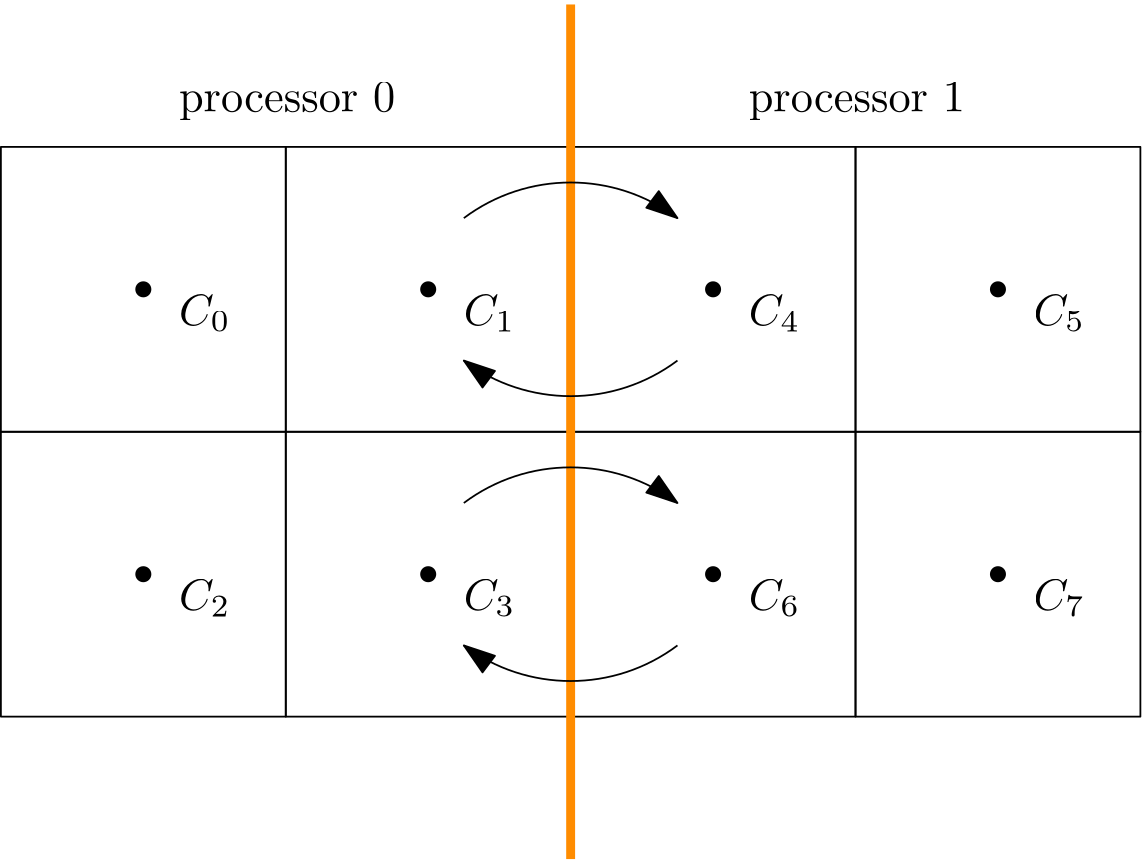
If this is the situation we have with MPI, i.e. we use two processors, and we have a domain split into two halves, where each processor is working on their own subdomain, we will need to exchange data at the interface, usually to compute our gradients, as we have seen previously as well. So now, we use MPI (the hint is in the name, i.e. Message Passing Interface) to pass data (messages) across the inter-processor boundaries (interface).
There are different ways in which we can achieve this, and we need to differentiate between two different types of message passing (memory transfer) approaches:
- Blocking vs. non-blocking communications
- Collective vs. point-to-point (non-collective) communications.
Let’s start with blocking communications. I recently came back home after spending 5 months abroad. Our neighbour was looking after our house, so it was still in good condition. However, as soon as I turned the electricity on, the internet was not working. Try as I might, I was not able to get it back online.
So, I called my internet provider, and they did some checks on their end but couldn’t figure out what was wrong. The lights on my router were not supposed to light up in the way they were, hinting at some deeper issue we would not be able to solve right then, and so the person booked an engineer to come round and have a look. During this call, the person on the other end was doing some checks, and whenever she was doing that, she would say those famous words we all love to hear: Please hold
During those brief 4-bar music-infused intermissions, when we are instructed to hold the line, what do you do? Leave the phone, go out and do the grocery shopping, or are you waiting with your phone glued to you, waiting for the other person to release you from 4 bar music hell? Probably the latter. You may do some small tasks like putting on the kettle, but you wouldn’t start to do anything more substantial.
(Oh, and if you wondered: Someone performed maintenance on the fibre optic cables in our estate and cut the cable to our house (by accident?!). The engineer who had to come out confirmed this, put a new cable in, and I was back online. I love the fact that someone cut the cables and then thought “Ah, fuck it, not my problem” …)
This is an example of a blocking communication. The other person has told us to wait for them, and we do. We wait for them to finish their task, and then we can, together, move on to the next task. In MPI, we do have blocking communications as well, where we tell two processors to collectively perform a communication and only continue with the computation once the communication has been completed.
Instead of blocking communications, we, as a society, have collectively embraced non-blocking communications. Emails, instant text messaging, chats, and Microsoft Teams (Microsoft is always in a category of its own!) are all examples of non-blocking communications. After you have made the effort of locating my email address at the bottom of this page and telling me how wrong I am about Imperial College, you go on about your day and don’t wait until I respond.
After some time, I may or may not respond, and once I do, you can choose to read the response immediately, or you can take your time as well. In MPI, non-blocking communications mean we initiate the data transfer but then immediately go on to perform some computation. We are essentially trying to overlap computations with communications and hope that the communication has finished (all data has been transferred) after we are done computing the solution on our private sub-domain.
We can mix and match blocking and non-blocking communications. A typical pattern within a solution update is as follows:
- Perform a non-blocking send operation at the beginning of the time step, where data for adjacent processors is sent, which they will need at some point.
- Perform computation on private sub-domain, excluding points directly attached to the inter-processor boundary, i.e. those that require information from adjacent processors.
- Perform a blocking receive operation, where we ensure that all data has been sent and received after we finish the receive operation.
- Update the cells near the inter-processor boundary, using the data we just passed around.
We will see this pattern in our 1D heat code in just a second. Before we do that, I also want to talk about collective and point-to-point communication. Imagine that you are working in a group of 5 people. You may have weekly meetings, where you come together as a group. These group meetings would be classified as a collective communication effort, i.e. all of you have to be present before you can start.
This means that if you are expecting everyone to attend, but only 4 of you are present at the specified start time, while the fifth person is sending apologetic text messages that they will run 15 minutes late, but they will definitely attend, you are left waiting 15 minutes. In that time, you may distract yourself with 15 minutes of doomscrolling, but you are not able to do anything productive (again, you wouldn’t leave to do your grocery shopping at that point).
In collective communications, we have to wait until everyone is available and has finished their task before we can continue. In our group example, you can only start with your group meeting once the fifth person has joined. In the context of MPI, a collective communication is one where each processor has to participate. If only one processor is not showing up, or coming late to the party because they were busy doing some computation, all other processors have to wait.
This is very costly, and it will quickly create a communication bottleneck for us. There are a few collective communications we need to perform, so we really want to make sure that we have good load balancing. If we don’t, then we will have processors waiting a lot of the time, which will destroy our parallel performance.
For example, when we compute the residual, we do that on each processor. But we need the information on all residuals on each sub-domain to compute the global residual for the user. In this case, we need to perform a collective communication at each time step. One optimisation that we can do here is to perform the residual exchange only every N iterations, where N may be 5 or 10. This can help to reduce the communication overhead of the parallel computation.
The best way to improve the performance of collective operations, though, is to make sure that each processor has an equal load, and the communications are otherwise minimised. If every processor comes to the collective communication point at the same time, then these communications aren’t that problematic.
The opposite of collective communications is point-to-point communications, which happens between two processors only. In the example we saw above with the two processors, we saw that we have a point-to-point communication between processor 0 and 1, which was both non-blocking (sending data) and blocking (receiving data).
With that out of the way, we are not ready to look at the MPI code. There will be quite a bit more code now due to MPI, and that is just the nature of it. There is quite a bit of boilerplate code we have to write because we are in charge of exchanging data. While this means that we have to write more code, it also provides us with the possibility to fine-tune and optimise our code. We get more control than, say, in OpenMP, which is great for getting the last bit of performance out of the code.
As we have done in the previous examples as well, I’ll give you the code first, and then we can look at some detailed explanations below the code. Try to read it first, though, and see what is happening before looking at the explanations.
#include <iostream>
#include <vector>
#include <chrono>
#include <fstream>
#include <string>

#include <mpi.h>

int main(int argc, char* argv[]) {
    // Initialise the MPI environment
    MPI_Init(&argc, &argv);

    // Get the number of processes
    int worldSize;
    MPI_Comm_size(MPI_COMM_WORLD, &worldSize);

    // Get the current processor ID (rank) of the process
    int rank;
    MPI_Comm_rank(MPI_COMM_WORLD, &rank);

    // input parameters
    const int numberOfPoints = static_cast<int>(atoi(argv[1]));
    const double leftBoundary = 0.0;
    const double rightBoundary = 1.0;
    const double CFL = 0.25;
    const double heatDiffusionCoefficient = 0.01;
    const double finalTime = static_cast<double>(atof(argv[2]));

    // computed input paramters
    const double dx = 1.0 / (numberOfPoints - 1);
    const double dt = CFL * dx * dx / heatDiffusionCoefficient;
    const int numberOfTimeSteps = static_cast<int>(finalTime / dt);

    // Domain decomposition
    int pointsPerProcess = numberOfPoints / worldSize;

    if (rank == 0) {
        std::cout << "Number of processes: " << worldSize << std::endl;
        std::cout << "Number of points per process: " << pointsPerProcess << std::endl;
    }
    MPI_Barrier(MPI_COMM_WORLD);

    // check that we have a valid decomposition. If we don't, then add additional points to the last processor
    int pointsNotUsed = 0;
    if (rank == worldSize - 1) {
        const int totalPoints = worldSize * pointsPerProcess;
        pointsNotUsed = numberOfPoints - totalPoints;
        pointsPerProcess += pointsNotUsed;
        if (pointsNotUsed > 0) {
            std::cout << "Adding " << pointsNotUsed << " point(s) to last processor" << std::endl;
        }
    }

    // allocate memory for field arrays
    std::vector<double> T0(pointsPerProcess); // T at time n
    std::vector<double> T1(pointsPerProcess); // T at time n+1
    std::vector<double> x(pointsPerProcess);

    // create mesh
    for (int i = 0; i < pointsPerProcess; ++i) {
        x[i] = dx * (i + rank * (pointsPerProcess - pointsNotUsed));
    }

    // initialise field arrays
    for (int i = 0; i < pointsPerProcess; ++i) {
        T0[i] = 0.0;
        T1[i] = 0.0;
    }

    // set boundary conditions (important, set it for T1, not T0)
    // only set it for left-most processor (rank == 0) and right-most processor (rank == worldSize - 1)
    if (rank == 0) {
        T1[0] = leftBoundary;
    }
    if (rank == worldSize - 1) {
        T1[pointsPerProcess - 1] = rightBoundary;
    }

    // helper variables for MPI
    std::vector<MPI_Request> requests;
    double leftBoundaryValue = 0.0;
    double rightBoundaryValue = 0.0;

    double startTime = MPI_Wtime();
    // loop over all timesteps
    for (int t = 0; t < numberOfTimeSteps; ++t) {
        T0 = T1;

        // send data to the right processor (except for the last processor, as there is no processor to the right)
        if (rank < worldSize - 1) {
            requests.push_back(MPI_Request{});
            MPI_Isend(&T0[pointsPerProcess - 1], 1, MPI_DOUBLE, rank + 1, 100 + rank, MPI_COMM_WORLD, &requests.back());
        }

        // send data to the left processor (except for the first processor, as there is no processor to the left)
        if (rank > 0) {
            requests.push_back(MPI_Request{});
            MPI_Isend(&T0[0], 1, MPI_DOUBLE, rank - 1, 200 + rank, MPI_COMM_WORLD, &requests.back());
        }

        // compute solution at next time level T^n+1 using an explicit update in time and e central difference in space
        for (int i = 1; i < pointsPerProcess - 1; ++i) {
            T1[i] = T0[i] + heatDiffusionCoefficient * dt / (dx * dx) * (T0[i + 1] - 2 * T0[i] + T0[i - 1]);
        }

        // before we try to receive data, we should make sure that the send requests have completed
        MPI_Waitall(static_cast<int>(requests.size()), requests.data(), MPI_STATUSES_IGNORE);

        // receive data from the left processor (except for the first processor, as there is no processor to the left)
        if (rank > 0) {
            MPI_Recv(&leftBoundaryValue, 1, MPI_DOUBLE, rank - 1, 100 + rank - 1, MPI_COMM_WORLD, MPI_STATUS_IGNORE);
        }

        // receive data from the right processor (except for the last processor, as there is no processor to the right)
        if (rank < worldSize - 1) {
            MPI_Recv(&rightBoundaryValue, 1, MPI_DOUBLE, rank + 1, 200 + rank + 1, MPI_COMM_WORLD, MPI_STATUS_IGNORE);
        }

        // now use the received values to compute the values at the inter-processor boundaries
        if (rank > 0) {
            int i = 0;
            T1[i] = T0[i] + heatDiffusionCoefficient * dt / (dx * dx) * (T0[i + 1] - 2 * T0[i] + leftBoundaryValue);
        }

        if (rank < worldSize - 1) {
            int i = pointsPerProcess - 1;
            T1[i] = T0[i] + heatDiffusionCoefficient * dt / (dx * dx) * (rightBoundaryValue - 2 * T0[i] + T0[i - 1]);
        }
    }
    double endTime = MPI_Wtime();
    double duration = endTime - startTime;
    if (rank == 0) {
        std::cout << "Executation time: " << duration << " seconds" << std::endl;
    }

    // compute error
    double error = 0.0;
    for (int i = 0; i < pointsPerProcess; ++i) {
        error += std::abs(T1[i] - x[i]);
    }
    error /= numberOfPoints;

    // reduce error over all processes into processor 0 (the root processor)
    int root = 0;
    double globalError = 0.0;
    MPI_Reduce(&error, &globalError, 1, MPI_DOUBLE, MPI_SUM, root, MPI_COMM_WORLD);

    // print error on processor 0 (the only processor that knows the global error)
    if (rank == root) {
        std::cout << "Error: " << globalError << std::endl;
    }

    // reconstruct the global temperature and coordinate array so that it can be written to disk by just one processor
    std::vector<double> globalTemperature;
    std::vector<double> globalX;
    if (rank == root) {
        globalTemperature.resize(numberOfPoints);
        globalX.resize(numberOfPoints);
    }

    // store the number of points that are send by each processor in an array
    std::vector<int> pointsPerProcessArray(worldSize);
    MPI_Gather(&pointsPerProcess, 1, MPI_INT, &pointsPerProcessArray[rank], 1, MPI_INT, root, MPI_COMM_WORLD);

    // store the offset/displacement, which states the starting point into the global array for each processor
    // for example, with 3 processors, where processor 0 send 3 elements, processor 1 sends 5 elements, and processor 2
    // sends 1 element, the offset/displacement array is [0, 3, 8]. Processor 0 will write at location 0 in the global
    // array, processor 1 will write at location 3 in the global array, and processor 2 will write at location 8 in the
    // global array
    std::vector<int> offsets(worldSize);
    if (rank == root) {
        offsets[0] = 0;
        for (int i = 1; i < worldSize; ++i) {
            offsets[i] = offsets[i - 1] + pointsPerProcessArray[i - 1];
        }
    }

    // start gathering all data into the root processor
    MPI_Gatherv(&T1[0], pointsPerProcess, MPI_DOUBLE, &globalTemperature[0], &pointsPerProcessArray[0], &offsets[0], MPI_DOUBLE, root, MPI_COMM_WORLD);
    MPI_Gatherv(&x[0], pointsPerProcess, MPI_DOUBLE, &globalX[0], &pointsPerProcessArray[0], &offsets[0], MPI_DOUBLE, root, MPI_COMM_WORLD);

    // output results on the master processor
    if (rank == root) {
        auto finalTimeString = std::to_string(finalTime);
        finalTimeString = finalTimeString.substr(0, finalTimeString.find("."));
        std::string fileName = "results_MPI_" + finalTimeString + ".csv";
        std::ofstream file(fileName);
        file << "x,T" << std::endl;
        for (int i = 0; i < numberOfPoints; ++i) {
            file << globalX[i] << ", " << globalTemperature[i] << std::endl;
        }
        file.close();
    }

    // Finalise the MPI environment.
    MPI_Finalize();

    return 0;
}Jepp, MPI is a little bit more involved, so let’s go through it step by step:
- Line 7: Starting off easy, first, we include the MPI header file to ensure that we can use it.
- Line 11: We have to tell our program that we want to use MPI. To do so, we call the
MPI_Init()function, and we forward the command line arguments here so that each processor is aware of any potential arguments. If we don’t have any command line arguments to pass, then we can also writeMPI_Init(NULL, NULL). - Lines 14-15: One of the first things we want to know is the number of cores that are available. We do that by calling the
MPI_Comm_size(). This function is expecting two arguments. The first is the communication group, and we always getMPI_COMM_WORLDby default (which we will use throughout this program).
When we launch our MPI program, we tell it how many cores to use. MPI will then allocate the requested number of cores to your program and store them in theMPI_COMM_WORLDgroup. For example, if you have a 12-core PC but only use 4 cores, you need to know which 4 cores out of the 12 work on the MPI program. We need to know that so that we can later send messages between these (and that we don’t send messages to a processor that doesn’t participate in the program).
MPIC_COMM_WORLDknows which cores participate and will ensure we send data to the correct processor. We can create our own communicators (for example, we can split the 4 cores that we have and create two groups of 2 processors each, where one group computes some CFD results while the other group looks after structural simulations for Fluid-Structure interaction (FSI) simulations, for example).
The second argument,wordlSizeis the variable in which we store the results. Since we store the results directly in this variable, we have to pass it in by reference (using the address-of operator&), which will ensure any modifications made to that variable within theMPI_Comm_worldcall will persist after the function has finished executing. - Lines 18-19: We do something similar here to the previous call, except that we now look for the processor ID within the
MPI_COMM_WORLDcommunicator. If we run our program on 4 cores, then each core will independently run our code from line 11 (when we callMPI_Init()). Once we reach line 19, we will identify which processor ID has been assigned to us, which we can then later use to assign data to a specific processor, as well as to establish communications between two specific processors. In OpenMP, a processor is called a thread; in MPI, we refer to them as ranks. I’ll use the same naming convention here. - Line 35: We have a 1D problem, so our domain decomposition is as simple as taking all the points that we have in our simulation and dividing them by the number of processors that we have, i.e. the variable we determined on line 15 when calling
MPI_Comm_world(). In case the number of points is not divisible by the number of processors, we have to do some additional work, which we will do on lines 44-52. - Lines 37-40: By convention, processor ID 0 (or rank 0) is the so-called master processor. Whenever there is work to be done by just a single processor, it is the master who is performing all of this work. MPI has used for quite some time the unfortunate terminology that rank 0 is the master, and all other participating processors are slaves, but there seems to be (finally) a shift towards avoiding the word slave, and the term worker is more commonly used nowadays.
In any case, we assign rank 0 as the master so that, in theory, we could also run our MPI program with just a single core. Here, I am just printing the number of processors and points per processor. - Line 41: I am now making a collective call to
MPI_Barrier(). This call will ensure that all processors have arrived at this point before continuing. To be honest, there is absolutely no point in having this call here, but I wanted to show you the syntax in at least one place so you have seen it once. However, if we look at the 4 preceding lines, we can imagine a situation in which rank 0 may do some checks, which may fail, resulting in rank 0 terminating execution prematurely. Now we have all other processors waiting at the barrier, and they will never be able to proceed, because rank 0 won’t arrive. This would be a classical deadlock situation. - Lines 44-52: We did our domain decomposition on line 35, but as alluded to before, we may have a situation where we can’t cleanly divide the number of points by the number of participating processors. There are several ways of dealing with it. What I am doing here is to check how many points have not been accounted for, and then add those points to the last processor. So, if we have 24 points and 7 processors, each processor receives 3 points. 7\cdot 3 = 21, so there are 24 - 21 = 3 points not accoutned for. These are now added to the last processor with ID
worldSize - 1. The minus 1 is there because our processor IDs start at 0, not 1. - Lines 55-57: We allocate now arrays based on the number of points per processor, no longer for the entire domain. Remember that MPI is a distributed memory approach, and so we allocate only memory for our specific processor. Also, the variable
pointsPerProcessormay not be the same for each processor. We saw on line 44-52 that the last processor may have a different value forpointsPerProcessor. This can be confusing, especially when you get started with MPI. - Lines 60-62: Now we create the mesh. The mesh needs to go from 0 to 1. However, each sub-domain has its own mesh section. For example, if we have 4 processors, the mesh for rank 0 will go from 0 to 0.25. The mesh for rank 1 will go from 0.25 to 0.5, and so on.
If I only multiplied the loop variableiby the global spacingdx, all of my sub-domains would go from 0 to 0.25 (using the same example values as before). Therefore, I need to offset the loop variableiby the number ofpointsPerProcessor, which will ensure that each subsequent processor will start at 0.25, 0.5, and 0.75, instead of starting again at 0.
ThepointsNotUsedneeds to be subtracted. Only the last processor sets this value, so for all other processorspointsNotUsedis zero. If we did not do this subtraction, the last processor would think that all other processors had the same number of points as itself, and so it would compute the offset at which point to start incorrectly. - Lines 72-77: Now we are setting the boundary conditions. We only want to set it for the left-most processor (rank 0) and the right-most processor (worldSize – 1). If we didn’t, then each processor would set a boundary condition at their inter-processor boundary, i.e. somewhere in the middle of the domain, which we don’t want.
- Lines 80-82: We are setting up some helper variables that we will use for our MPI communications. The left and right boundary values will be used to store received data from each processor. That is, we will receive data from our right neighbour processor into our
rightBoundaryValuevariable, and data from our left neighbour processor into ourleftBoundaryValuevariable.
We also have astd::vectorof typeMPI_Request, which we will need to use later. When we do our non-blocking communications, we don’t know at what point they have completed. When they do complete, this request vector will reflect that, and so we can check this request vector later to ensure that all communications have been completed before we start to do anything with the received data. - Line 84: We create a timestamp of our starting time using MPI’s
MPI_Wtime(), or wallclock time. This is similar to thestd::chronocall we had before, but MPI provides its own timing functionality. We can usestd::chronoinstead, but then we would have to fence it off again with aif (rank == 0) { ... }call. It is common to just use the MPI internal timing here instead. - Line 87: In OpenMP and CUDA, we saw that the temperature array update (storing T<sup>{n+1} computed at the previous time step in T</sup>n) was done in parallel. In MPI, we have a distributed memory approach, and so each processor will have their own private copy of
T1andT0, and so we can simply copy the entire content ofT1inT0, just as we did in the sequential program. - Lines 90-93: This is our first communication. We first ensure that we are not on the right-most processor (
rank < worldSize - 1), as we want to send data to our right neighbour processor. The right-most processor won't have a neighbour to its right.
We are using the non-blockingMPI_Isend()call here, where theIstands for immediate (although I have seen a few different definitions for it as well, immediate makes most sense in my books). In general, whenever we see a capitalIin an MPI function call, i.e.MPI_I..., it means that this is a non-blocking call. The corresponding blocking call would be without theI. For example, a blocking send call would beMPI_Send().
Let's look at the 7 different parameters that go into an MPI send call. The first argument is the data we want to send. If we want to send more than just a single value, like an array, we specify the start location of that array. In this example, we want to send the last element in ourT0array, which should be sent to our neighbour to the right. The next argument specifies how much data I want to send. I only want to send a single element, so I can put a1as the second argument. The third argument specifies the type I am sending, which are typically preceded by anMPI_. In this case, I am sending adouble, soMPI_DOUBLEis the type.
The fourth argument tells MPI which processor should receive this data. In our case, we want to send data to the right processor, which has a rank ofrank + 1. So, for example, if I am on processor 1 withrank = 1, then the processor to my right isrank = 2. So, by saying I want to send data torank + 1, I am selecting the processor to my right automatically.
The fifth argument is a tag. In this example, we are just sending a single element to my processor on the right, but imagine I am solving the Navier-Stokes equation and I want to send velocity, pressure, temperature, and density to the processor on the right. I need to be able to distinguish each send operation, so the received data can later be correctly identified. This is what the tag is doing, and we typically give some identifying number + some combination with therankitself.
Here, I am using100as my identifying number, and, if I also send velocity, pressure, and density information, I may bump these up to200,300, and400, respectively. In this way, I can later identify what data was sent. Since I am also using therankhere to compute a tag, I need to be careful. If I use more than 100 processors, I may have something like100 + rank, which can now become larger than200, then may send data into the wrong array.
For that reason, it makes sense to bundle all data you want to send into its own container and then send that container instead. This makes the tag computation less error-prone, but also means that you have to tell MPI about your custom data classes, which is not necessarily straightforward (but support exists for that in MPI).
After the tag, we tell which communicator we want to use, and usually we always use the default communicator, i.e.MPI_COMM_WORLD. Finally, we have to pass a reference to the last element in ourrequestvector, holding ourMPI_Requestdata. We just created an empty instance of that on line 91, and now we tell MPI that it should put all information about the communication into this array. We can then later check if this specific communication has finished. - Lines 96-99: This is exactly the same as lines 90-93, except that we now make sure that the first processor is not included in this call (
rank > 0), as we want to send now data to our left-most processor (and the first processor won't have a neighbour to its left). We are now sending the first element of ourT0array. We still only send 1 element of typeMPI_DOUBLE, but now we are sending it to the left processor, so we are sending it torank - 1. The tag is now using an identifying number of200and we add therankto it. The communicator group is stillMPI_COMM_WORLDand we use the samerequestvector here to add one additionalMPI_Requestobject. - Lines 102-104: We have prepared the non-blocking communication, and that process has started in the background. We can now update the rest of the temperature array at the next time level T^{n+1}. Notice that our loop starts at
i = 1and it goes topointsPerProcessor - 1, i.e. we are not yet updating the values on the inter-processor boundaries, which are located ati = 0(as long as we are not on the left-most processor) andi = pointsPerProcess - 1(as long as we are not on the right-most processor). - Line 107: We have initiated the communication with two non-blocking send communication calls, and we have updated all the internal variables. Now we want to compute the final values on the inter-processor boundaries. In order to do that, we need to ensure that all data was received from the send call. Thus, on line 107, we call the
MPI_Waitallfunction, which first asks us how many requests we should check. I am using the size of the request object here, because we don't know how many requests we should check. If I have one processor to my right and one to my left, then I will have made 2 non-blocking sends to the left and right, and so my request object will have a size of 2. But if I am on the left or right domain boundary, then I will have to send data to one processor, and my request vector will have a size of 1. For that reason, we can't just use a value of 2 here and instead need to find it dynamically.
The second argument intoMPI_Waitall()isrequest.data(), which is the raw pointer of each element of astd::vector. MPI is written in C, not C++, and so it doesn't understand containers likestd::vectors. We need to give it raw pointers which a C program can understand, and that is what the call todata()achieves.
We could also check the status with the third argument, which we may want to do if we have a more complex code and we check at a few points if the data has been received, instead of only doing that at the end. Since we don't really care and want to wait until all data has been received, we ignore the status report withMPI_STATUSES_IGNORE. - Lines 110-112: We now do the reverse of a send call and instead receive data with the
MPI_Recv()function call. This is a blocking communication. There is also an equivalent non-blocking communication, calledMPI_Irecv(), though there is no advantage of pairing two non-blocking communications over one blocking and one non-blocking communication. If we used a non-blocking communication here, we would have to generate an additionalstd::vectorvector and callMPI_Waitall()again before proceeding, so we may as well just use a blocking call here.
Remember, we used a non-blocking call for the send so that we could do some additional stuff in the meantime, like updatingT1on line 103. But since there is nothing else for us to do at this point, using a blocking or non-blocking call here will have no measurable difference.
We use the samerank > 0check here to ensure that we are not on the left-most processor. If that is the case, we know that there must be a processor to our left (rank - 1) which has sent some data for us. We want to now receive this data, which we will store into the variable that is given as the first argument to theMPI_Recvcall, hereleftBoundaryValue. We pass the address of the variable again, so that MPI can update the value found at that address so thatleftBoundaryValuewill contain the received value after MPI has finished its communication.
The second and third arguments are the same as in the corresponding send call, i.e. we are sending one element of typeMPI_DOUBLE. The fourth argument tells us where the data should be coming from. In this case, it is coming from our left neighbouring processor, so it is coming fromrank - 1.
We have to compute the correct tag as the fifth argument. On line 92, we saw that we send data to our right processor (which is the value we are now receiving on line 111 from our left processor). The tag on line 92 was100 + rank. If processor 2 sends data to processor 3, then the tag was102. When processor 3 receives the data, the tag must be100 + rank - 1, i.e. in our example100 + 3 - 1 = 102. We simply ensure that we are setting the correct tag value here so that we receive the right data.
We use the default communication group again, i.e.MPI_COMM_WORLD, and we can ignore the status withMPI_STATUS_IGNOREas this is a blocking receive operation. - Lines 115-117: This is the same call to the previous lines, only now we are receiving data from the right processor, and so, we need to make sure that we are not on the right-most processor, which we do with the check
rank < worldSize - 1.
The only difference here is that we receive data now into therightBoundaryValue, we are receiving data from our right neighbouring processor, i.e.rank + 1, and we are computing the tag as200 + rank + 1, as the corresponding tag on line 98 was computed as200 + rank. - Line 122: We explicitly update the value at
T1[i]withi = 0using the receivedleftBoundaryValue. Originally, we hadT0[i - 1]here, but ifi = 0, theni - 1would result in an out-of-bounds memory request, crashing the program. But, withleftBoudnaryValuenow available, we can replace this value and manually update the value ofT1at the inter-processor boundary. - Line 116: We do the same as on line 122 here, only that we are updating
T1[i]withi = pointsPerProcessor - 1, i.e. the value on the right inter-processor boundary. The value ofT0[i + 1]is now replaced by the value we received into therightBoundaryValue. Once this is done, the current time step has finished, and we go back to the beginning of this loop. - Lines 130-134: Once the time loop has completed, we take another time stamp and compute the total time it took to run the time loop. We print this result to the screen as well on line 133 and use the same trick as before, where only rank 0 is printing this value.
- Lines 137-141: We compute the local error norm, just as we did in all of the other cases, but now we compute the error for each sub-domain separately. Thus, each processor computes an individual error.
- Lines 144-146: We need to collect all individual errors from each processor and compute the final error as a sum of all individual errors. This type of operation is quite common, where all processors compute individual parts, and then all processors send them to one processor, who then decides what to do with them. This type of operation is a so-called reduction operation.
We call theMPI_Reduce()function that is doing that for us. The first argument is the value we want to send from all processors. The third argument is the number of elements we are sending, and the fourth argument is the type again, hereMPI_DOUBLE. The fifth argument tells MPI what we want to do with the value. In this case, we want to sum up all elements. The result of this will be stored in the second argument, which here isglobalError.
There are other types of operations available, for example,MPI_PRODfor multiplying all individual contributions, orMPI_MAX/MPI_MIN, which select the maximum/minimum value computed on each processor. When we compute a stable time step on each processor, for example, we may want to find the maximum allowable time step and use that, for which we would useMPI_MAX.
The sixth argument tells MPI which processor should process all of that data. Here, I have defined a new helper variable calledroot, which I have set on line 144 to rank 0. The seventh and final argument, again, tells MPI which communication group to use. - Lines 149-151: If we are rank 0, then we print the global error on line 150, the one that we just reduced from all other processors.
- Lines 154-159: We now start to prepare the data output. For that, we define the first two arrays that are going to hold the temperature and coordinate arrays for the entire domain. If we are on the root processor, i.e. when
rank = 0, only then do we allocate memory for it. This array will now have as many entries as all processors combined. This is something we can do when we are dealing with simple 1D arrays to create a test program, where we now send all data to the root, or master processor, i.e. the one withrank = 0, but for more complex programs, we would likely make use of MPI's parallel I/O (input/output) capabilities and let each processor write its content to disk separately. - Lines 162-163: We define the
pointsPerProcessorArray, which will contain the number of points that each processor has in its sub-domain. We use theMPI_Gatherfunction, which is a collective communication. It is similar to theMPI_Reduce()call, in that all processors send one specific piece of information to one processor, typically the root/master. The only difference is that we are not adding up all individual elements; instead, we store them in an array, where each processor sends its contribution into the array, at the index that is equal to their rank. So, processor 0 will store their contribution at index 0 in the array, processor 1 at index 1, and so on.
We see that the first argument toMPI_Gather()is the value we want to send (we send one element of typeMPI_INT, i.e. see the second and third argument), and we store it in thepointsPerProcessorArrayat the index that is equal to the processor's ID (i.e. at indexrank). All of this information will be sent to the root again, which will be the only processor which will know about this information.
The reason we have to collect this data is that the last processor may contain more cells than other processors. We could have also done a send and receive call between the first and last processor, but I wanted to show you some additional MPI calls, likeMPI_Gather(), which are quite commonly used. - Lines 170-176: Based on the number of points per processor, we can now compute a so-called offset, or displacement vector. This will show at which index, in the global temperature and coordinate vector, each processor will start writing their data to. So, for example, if we had 3 processors, and the number of elements per processor would be
[3,4,2], then the offset, or displacement vector, would become[0,3,7]. That is, the first processor will write its data at index 0. The second processor has to skip the first 3 elements, because that is where processor 0 is writing, and so it will start putting its 4 elements from index 3. The final processor will have to jump over processors 0 and 1, which collectively write 7 elements, and so the final processor will have to start writing its data from index 7 (3 + 4). - Lines 179-180: Now that we have created the points per processor array, as well as the displacement vector, we can use the
MPI_Gatherv()function to collect all individual data from the processors and write it into the global temperature and coordinate array at their specific index. We use theGatherv, notGathervariant here, where thevat the end indicates that we have variable sizes that we are collecting.
When we usedMPI_Gather(), we collected the same amount of information from each processor, but withMPI_Gatherv()we collect an arbitrary amount of information from each processor.
The first argument is again the variable, or here the array, into which we want to receive data. We then state how many elements we want to send. Each processor may now have a different value forpointsPerProcessor. The type isMPI_DOUBLE, as the temperature and coordinate arrays are of typestd::vector.
The fourth argument tells MPI that we want to send the data to the global temperature and coordinate array, and the next two arguments are thepointsPerProcessorArrayandoffsetvector, which will tell MPI how many elements to write into the global arrays, and at which location we should start writing these for each processor. This is what we have just created in the previous lines of code. Only processor 0 will have this information available, as we have enclosed all previous calculations withif (rank == 0) { ... }. Thus, we have to make sure that theMPI_Gatherv()function gathers all of this information into processor zero, which we can see is the case.
The final three arguments are that we gather variables of typeMPI_DOUBLE, that it is indeed the root which receives all of the information, and that all processors participate in the blocking, collective communication. - Line 196: After we have written the content of the collected information out to disk as a
*.csvfile, we are done with MPI, and we can call theMPI_Finalize()command. Each program needs to call that, which signals the end of the MPI program. Afterwards, we can gracefully exit the program with a standardreturn 0call.
That was quite a bit to go through, and you may be wondering, is all of this code really required? Well, yes and no. What I have shown here is not necessarily the most efficient implementation. It is almost a universal rule that I can either show you how to use a framework, which will make it rather inefficient, or I can write really efficient code, but then it will be difficult to understand what I am doing.
Thus, writing code for education and performance purposes is very different. I wanted to be a bit more verbose with some of the function calls, but there are better ways of dealing with MPI here. For example, for a simple case like what we have seen here, where we use a structured grid with processors to my left and right, we can use a Cartesian parallelisation topology.
If we use this approach, we create a new communicator, instead of using the default MPI_COMM_WORLD, which will then know how to send data to the left and right. We no longer have to manually compute the left and right processor ID, and it will also know that for my right-most processor, there won't be a processor to its right, and it won't send data. We don't have to perform this check either. The same is true for the left-most processor.
If you want to explore this concept in greater depth, you can find a similar implementation of the heat diffusion equation, now in 3D, here.
So far, we have talked only about 2-sided communications, that is, we send data from one processor (side) to another processor (side). However, we can also use one-sided communications, which are gaining popularity. In this approach, each processor allocates a dedicated memory area into which other processors are allowed to write. They can come, leave their data here, and go, without the other processor that is receiving this data needing to participate in this exchange.
This is akin to your Amazon delivery driver leaving your delivery outside your door when you are not home; it is a one-sided delivery in which you did not take part (open the door and take possession of the package). Because it is one-sided, there is potential to speed up communication times significantly, and hence we see this paradigm being used more and more.
So, if we want to get this beauty to run, we need to prepare our machine first. We need to get some form of MPI distribution onto our PC before we can compile and execute the code. On Windows, well, we have to install Microsoft MPI, it's not like we have a lot of choice here (although we can also use/try for free third-party implementations like Intel MPI or IBM MPI)
On UNIX, we have a bit more support that natively integrates with our operating system. The two most popular distributions are MPICH and OpenMPI (not to be confused with OpenMP, which I thought for a very long time was one and the same, just with a typo ...). We can install them with our favourite package manager, i.e. apt, homebrew, yay, etc.
Once we have done that, we can add the following lines to our CMake project:
# --- MPI ---
add_executable(heat1DMPI "src/heat1DMPI.cpp")
find_package(MPI REQUIRED)
target_link_libraries(heat1DMPI PRIVATE MPI::MPI_CXX)We define the executable and which source file it depends on, which we need to find the MPI installation; otherwise, we can't continue, and then we link our executable against the MPI library. And that's it, short and painless, well, at least this part of the compilation.
We can compile our project as before using CMake:
cmake -DCMAKE_BUILD_TYPE=Release ..cmake --build . --config ReleaseExecuting the solver is slightly different from before. On Windows, using Microsoft MPI, we have to use the following:
mpiexec.exe -n 4 .\heat1DMPI.exe 101 100We use the mpiexec.exe function here, which will launch our program. We provide it here with the command line argument -n 4, which means that we want to run our code with 4 processors in total.
Afterwards, we can specify the executable with its command line arguments just as we have done before.
On UNIX, you may write something like this:
mpiexec -n 4 heat1DMPI 101 100Here, we have simply removed the *.exe extension from both the executable and the mpiexec command.
There are, in-fact, two executables we can use to launch our MPI program, the second one is mpirun, which does not seem to be available in Microsoft MPI. However, on UNIX, depending on your installed MPI framework, you should also be able to use mpirun as:
mpirun -np 4 heat1DMPI 101 100Using mpirun usually requires using -np 4 instead of -n 4. These are the only differences, and it seems to be down to preference which one you use.
You will find both in the wild, so I thought I would mention it here for completeness. Congratulations, you survived your crash course into code parallelisation. We have come a long way; let us now find out how good our parallelisations are when we benchmark them against one another. We'll do that in the next section.
Case study: Comparing speed-up for different parallelisation strategies
In this section, I want to compare the different parallelisation strategies and see how they compare against one another. The first thing we should be doing is to make sure that all of the codes produce exactly the same results, and that the results they do produce are physically correct.
The following image shows all parallelisation strategies, including the sequential code, using different markers. I have plotted the results at three separate times, and each time uses a separate colour.
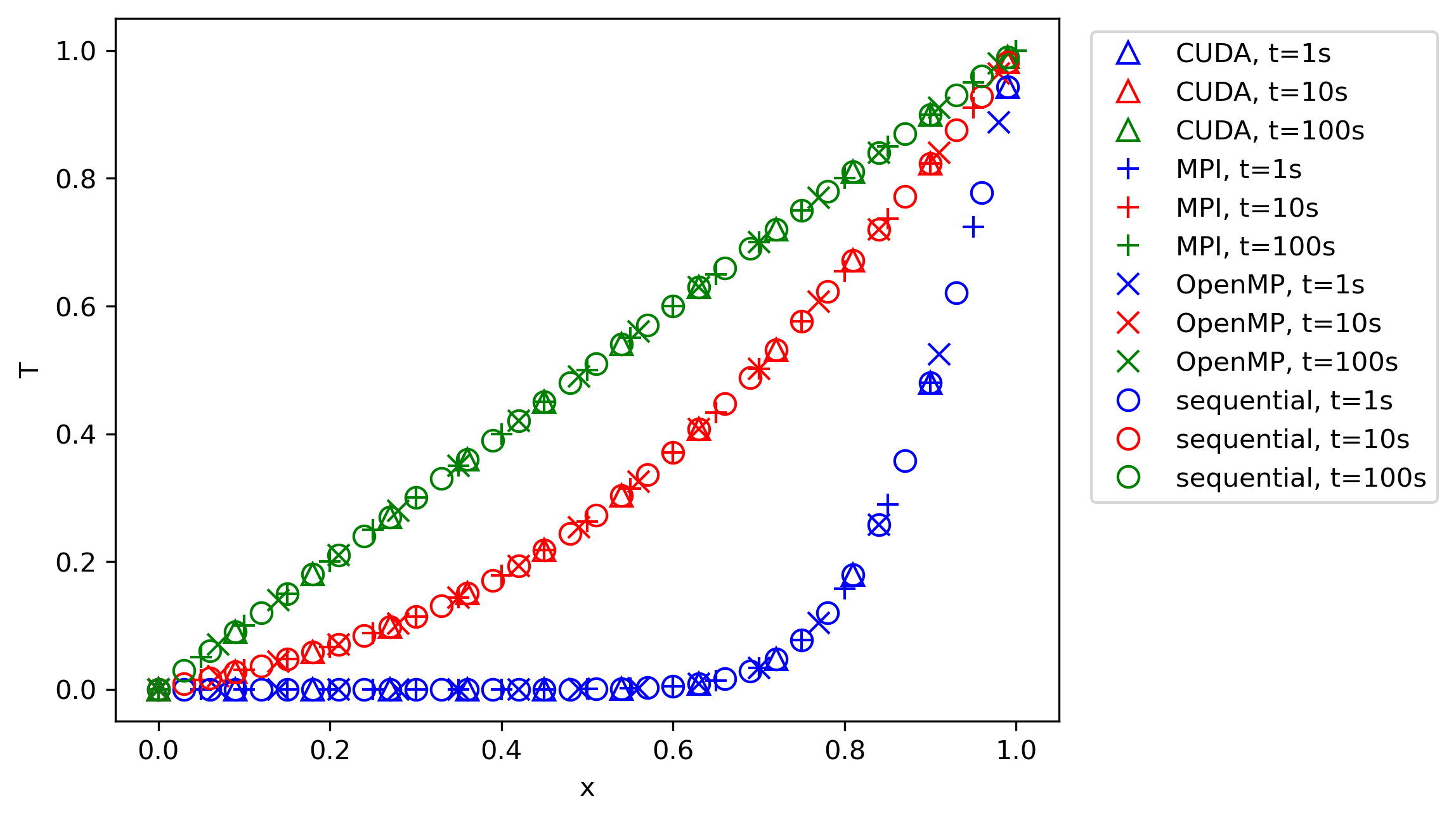
From this figure, we can infer that all parallelisation approaches provide the same result as the sequential code, and, as the time goes to a very large value, we reach the correct physical behaviour. We could use an analytic solution now to compare our results against; however, we can also use physical intuition to validate our results.
If the boundary conditions are such that the temperature is 0 on the left boundary and 1 on the right boundary, then we would expect to have a linear distribution of the temperature within the domain. After 100 seconds, this is exactly the phenomenon we see. In between, the solution gradually approaches this state, and we see how the temperature profile develops to this linear distribution.
So, in terms of correctness, we can state that all approaches seem to produce the correct physical behaviour. I have also computed the error norms (as we have seen in the codes before), and while I do not show them here, they are also all identical to within rounding errors.
Ok, so let's try our parallelised programs and see how they compare. I will use 1001 grid points in the domain, and I will let the solution run until a time of 100 seconds has been reached. At that point, the solution will have converged to a steady-state solution, as we have seen in the previous plot.
The table below shows the computational time for each approach. We have the time for the sequential code as well, which we are trying to beat. For OpenMP and MPI, we see the number of cores and how these affect the computational time. On the GPU side, I am using a single GPU to compute the solution.
If I wanted to use more than that, I would have to use MPI and CUDA together, where we have as many MPI processors as CUDA-capable GPUs, and all that these MPI cores would do is to communicate data between GPUs. This is slightly more involved and beside the point here in our introductory example, but if you want to use more than a single GPU, you will need to combine MPI and CUDA.
Without further ado, let us look at the computational results:
| CPU cores | GPUs | Sequential | OpenMP | MPI | CUDA |
| 1 | 0 | 0.126 | 0.207 | 0.228 | - |
| 2 | 0 | - | 0.305 | 34.8 | - |
| 4 | 0 | - | 0.406 | 78.0 | - |
| 8 | 0 | - | 0.563 | 132.2 | - |
| 0 | 1 | - | - | - | 4.18 |
Brilliant, so the sequential code takes 0.126 seconds, while MPI and OpenMP cannot reach a better performance than 0.2 seconds and above. Even worse, on 8 cores, MPI takes 132.2 seconds. CUDA takes over 4 seconds.
What this table shows is that everything we have just discussed is a lie, parallelisation slows down your code, and I have wasted 10 years of my life learning about different parallelisation approaches. Or is it?
Let's look at the numbers closer. We see that using more cores, either with MPI or OpenMP, will increase the computational cost. While MPI certainly shows a drastic explosion in computational cost, OpenMP is more moderate, yet it is still noticeable.
We are using 1001 points here in our domain, meaning that if we use 8 cores in total, each domain will get about 125 elements to work on. Having 8 cores means that we have to exchange information between 8 processors. So, as the number of processors reduces, we have less work to do per processor, but we also have more communications to do because there are more processors. Both of these effects will dramatically increase the time spent on communications, and thus, we see a significant increase in total computational time using MPI.
Why does OpenMP not suffer from the same issue as badly? Well, it is a shared memory approach, and so we don't have to send individual data between processors; they can all see the same memory and read and write to it. The reason OpenMP's computational time increases is just from the overhead of having to manage a parallel region.
After each #pragma omp for, we have an implicit barrier, meaning that all processors have to reach it together before they can continue. If you meet with your best friend at 6 pm, how likely is it that both of you arrive on time? What about if you meet with 10 friends? Do you think it is equally likely that everyone will arrive on time? Probably not, and the same is true for parallelisations.
Threads, or processors, will arrive at implicit barriers at different times, and the more you have, the more chances there are that just a single processor will hold you up, and so the computational time increases slightly.
Remember what we said earlier about good efficiency in CFD solvers. I said that commercial CFD codes can scale well down to 50,000 cells per processor, and for each cell, we may perform a few computations, not just a single temperature update (we may compute pressure, temperature, density, and momentum, and potentially several times per time step using an implicit system of equations).
We are now trying to parallelise a code which, in our example, has as few as 125 cells per core. We can't expect good scalability in this case; communication will just be too expensive. Even worse, in this example, most of the cost is spent updating the solution in time. We go all the way to 100 seconds, and so our loop over space contains relatively few elements (1001), while we have to perform many iterations in time to get to 100 seconds.
If we truly want to test our parallelisation, we really need to increase the computations per processor, which means we need to increase the number of points per processor significantly. How about 100 million points in total? That should do. However, since we are using an explicit time integration, we will be limited by our CFL number, and so our time step will become very small. Instead of going back to 100 seconds, let's do a very small time increment, so that we really spend most of the time computing, not communicating.
An end time of 1e-12 seems to work fine after some experimentation. This will mean that the solution itself will have barely updated, and so any attempt to compare it against the solution once the temperature has developed is pointless, and thus, the error we compute will be high. However, we are doing this now to test the parallelisation itself; we already know that the code works correctly.
The results for this end time using 100 million points (in total) are shown below:
| CPU cores | GPUs | Sequential | OpenMP | MPI | CUDA |
| 1 | 0 | 50.6 | 61.2 | 55.7 | - |
| 2 | 0 | - | 42.8 | 43.3 | - |
| 4 | 0 | - | 30.4 | 34.3 | - |
| 8 | 0 | - | 26.1 | 27.8 | - |
| 0 | 1 | - | - | - | 5.48 |
We see that the sequential code took 50.6 seconds now to compute. While both OpenMP and MPI show that they still require more time on a single processor, mainly due to all of the additional overhead of setting up the communications, they do start to reduce the computational cost as we increase the number of cores.
The following table shows the computed speed-up and efficiency of both OpenMP and MPI compared to the sequential code:
| Number of Cores | OpenMP | MPI | ||
|---|---|---|---|---|
| Speed-up | Efficiency | Speed-up | Efficiency | |
| 1 | 0.83 | 0.83 | 0.91 | 0.91 |
| 2 | 1.18 | 0.59 | 1.17 | 0.58 |
| 4 | 1.66 | 0.42 | 1.48 | 0.37 |
| 8 | 1.94 | 0.24 | 1.82 | 0.23 |
What we really care about here is the efficiency. It tells us how well we utilise our hardware to speed up our code. From the two previous tables, we see that we get barely about a speed-up of 2 using 8 cores, which is a pretty poor parallelisation.
This shows that explicit 1D code examples are difficult examples for parallelisation, as we are not spending enough time computing a solution, but rather communicating data between processors. However, if you go back to the discussion of Amdahl's law earlier in this article, we saw that getting good scalability is really difficult, and so for to demonstrate that, 1D code examples are actually quite useful to make this pain very visible.
What about CUDA? Those results are almost the same compared to the 1001 number of points and an end time of 1e-12. This shows that CUDA, once the setup time has been accounted for, can scale really well across problem sizes. Once we saturate our GPU with enough work, it can work on it really efficiently, and this is one of the reasons we like to use it in parallel computing.
In CFD applications, we typically require a lot of memory (RAM) to fit large problems into it. While this used to be a problem in the past, when we started experimenting with consumer hardware GPUs (opposed to dedicated computing GPUs, which don't even come with HDMI outputs for monitors, as they are supposed to be used for computing only), the generative AI bubble has seen companies making massive investments into computing GPUs with an abundance of memory.
While it appears that the current AI bubble will burst (again ...), which ushered in a lot of investment into GPU hardware and computing facilities, it means that there is an opportunity for GPUs to be used for CFD applications on the cheap in the future, once new avenues are explored of how these can be used elsewhere.
Therefore, learning GPU parallelisation is a worthy route, not just in case the AI bubble bursts, but also due to a lot of companies making a transition to GPUs, some more serious than others. But one thing is clear: GPUs are here to stay and will become even more important in the future for CFD applications!
Hopefully, you have gotten a taste now for how parallelisations work, and you are familiar with performance bottlenecks like Amdahl's law and the need to really have a lot of computations to be performed in the first place before utilising parallelisations.
Challenges in code parallelisation for CFD applications
Before we finish this article, I want to discuss a few challenges we face when parallelising our code. In this section, I highlight some of the issues I think are worthy of consideration.
Parallelisations of multigrid solvers
Ah, multigrids! They hold a special place in my heart. I have had many, many long discussions with my PhD supervisor during my PhD time about their usefulness, either at university or the local indian restaurant near our university that served an excellent (and yet non-traditional) Chicken Tikka Masala. They have now closed, and we have not just lost an excellent restaurant, but also the perfect debating ground for niche CFD topics! In any case ...
While I believed (and still do) that multigrids are quite useful and should be used for CFD applications, my supervisor had some good arguments against them, which are all valid. But to me, the advantages still outweight the disadvantages (and the support for multigrids in solvers like Fluent, OpenFOAM, SU2 do back me up here), although it has to be said that multigrids do work best for pure elliptic partial differential equations, not a mix of elliptic and hyperbolic, as is the case for the Navier-Stokes equations.
The following figure demonstrates what a multigrid does:
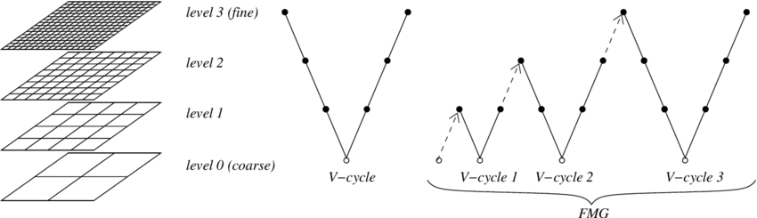
On the left, we see a couple of different grids (hence the name multigrid). On the top, we have the finest grid, and this is typically the grid that we have created with our mesh generator and read into our solver. The multigrid algorithm will now create a series of grids that have fewer cells on each level.
For example, if we had a 2D structured grid, as is shown in the example above, then we could combine 4 quad cells on the fine grid into a single quad cell on the next coarser grid. We then repeat the process by coarsening the grid until we only have a few cells left on the coarsest level, perhaps a few hundred or so.
Once we have all of these different grids created, we start computing our solution on them. First, we start on the finest grid level and compute the solution for a few iterations. Even though the solution may not have converged on the finest grid level, we take this intermediate result and interpolate onto the next coarser grid. This is known as the restriction step.
We repeat the same procedure on the next coarser grid, i.e. we compute the solution (now based on the solution from the finer grid) for a few iterations, and then restrict (interpolate) the result onto the next coarser grid, and so on. Once we have reached the coarsest grid and we have finished updating the solution on it, we start going up the grid hierarchy again.
We take the results from the coarsest grid and interpolate it onto the next finer grid. We compute the solution here for a few iterations and then go to the next finer grid. We repeat this until we have reached the final (finest) grid, which is the original grid we started with. Going from a coarse to a finer grid is known as the prolongation step.
SO why do we do this? There is a bit of theory behind multigrid, in which you can nicely show, mathematically, how a multigrid damps oscillations in your local error, but let's try to approach this from a more intuitive point of view. Imagine we are computing the pressure field (for which multigrids are typically used, as the pressure Poisson equation for incompressible flows has a pure elliptic character).
For an incompressible flow, changes in pressure are felt instantaneously everywhere in the domain (we could say that pressure changes propagate at an infinite speed, and this is a reasonable assumption as the propagation speed of pressure, i.e. the speed of sound, is typically much larger than the local flow velocities).
So, we have a pressure disturbance in one part of the domain, and we want to make sure its effect is felt everywhere in the domain. If we iterate now over our finest grid level only, then the speed at which the pressure would propagate is determined by the CFL number. The CFL number is just a non-dimensional measure of how much information propagates from one cell to another.
For example, if the CFL number is 1, then a particle travelling with the local flow velocity would move exactly one cell width or height per iteration. If the CFL number is 10, then it moves 10 cell widths or heights. I have discussed this in much more depth in my article on time stepping and the CFL number.
For the sake of argument, let's assume we use an explicit time-stepping algorithm. In this case, we are limited to using a max CFL number of 1. On the finest grid, it will take quite some time (iterations) before pressure changes are propagated everywhere in the domain. For example, if I am solving my flow on a square domain with 100 cells in the x and y directions, it would take 100 iterations with a CFL number of 1 to propagate pressure changes from the left to the right boundary. If my CFL number is less, this value will increase.
But now, let's bring our multigrid into play. Let's say we create 5 grid levels, where our original mesh had 100 cells in both the x and y direction. The next coarse grid may only have 50 cells in each direction. The next coarser grid will have 25 cells in each direction, the next coarser grid after that 12 cells, and the final grid only 6 cells in each direction.
If I now want to propagate the same pressure information from the left to the right boundary on the coarsest grid level, with a CFL number of 1, it will take me only 6 iterations, compared to the 100 iterations required on the finest level. Even better, the calculation on my now 6 by 6 grid will be much faster than my computations on my 100 by 100 grid.
So, we can now summarise the core idea behind a multigrid solver. We restrict our solution to coarser and coarser grids, so that we reduce the computational cost and allow the solution to propagate faster through the domain. This creates a solution on the coarsest grid that has taken care of all necessary propagations, but the solution will be inaccurate, due to the coarse nature of the grid. We then prolong our solution back onto the finest grid to get back accuracy, without having to worry about solution propagation speed.
Just as a sidenote: The way in which we chain restriction and prolongation steps together can be changed arbitrarily, but there are a few common patterns used in multigrids, commonly known as the V-cycle, W-cycle, or F-cycle, which are shown in the following (and yes, if you want to be excentric, you may invent your own cycle and assign it an arbitrary letter, this is, after all, how PhD titles are earned!):
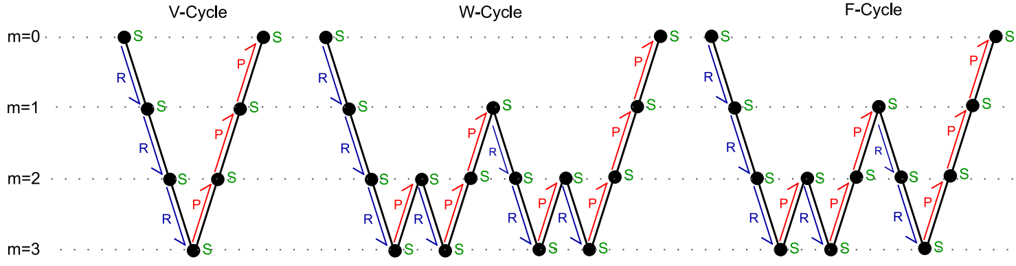
So, now that we have an understanding of multigrids, let's bring that into the context of parallel computing. We perform the domain decomposition on the finest grid. That is the grid we were reading into our solver, or generating as part of the simulation. That is the grid on which we want to have the final solution.
This presents a unique problem: Once we start to coarsen our grid, we start to reduce the number of cells per sub-domain. This then results in communication times to be much greater than the computational times on the coarser grid levels, as there is simply less to compute with fewer cells. Thus, the parallel efficiency for each subsequent coarser grid level becomes worse, and we may even end up in a situation where the multigrid, which is supposed to speed up the solution, may in fact slow down our total simulation time.
For large-scale problems, which require efficient utilisation of parallel resources, there are two common approaches:
- Become a parallel multigrid wizard, ideally the authority in the world for all questions related to multigrids, or, if that is difficult
- Avoid multigrids
The second option is, out of sheer practicality, the solution often employed. Common alternatives to the multigrid are Krylov subspace methods, which sound fancy, but you may know them better under the name of gradient-descent methods, such as the Conjugate Gradient method (which is by far the most popular method in this space).
That is not to say that people are not using multigrids. ANSYS Fluent makes use of multigrids even for the largest cases it can run. Their multigrid must have received a lot of attention. OpenFOAM allows you to use multigrids, but thus far, I haven't been able to see conclusive results demonstrating that it is just as efficient as Fluent when it comes to parallel efficiency.
Krylov subspace methods make your life a lot easier, so it is a good place to start. And, if you are writing your own code and you don't care about parallelisation (yet, you will eventually, I can promise you that!), there are plenty of easy-to-use libraries that ship with everything you'll need to use one of these methods. In C++, there are even a few header-only libraries, which make their usage particularly easy. My favourite: Eigen.
We don't speak of PETSc around here. The library, while capable for linear algebra applications, including a good range of Krylov subspace methods, follows a broken software development philosophy, meaning you are locked in and have to use software development tools that were developed a few decades ago, and have definitely stopped in development. If there were such a thing as a use by date, we would be long past that. It is only coincidental that I first had to use this software when I was at Imperial College ...
So, multigrids are really powerful, but they come with strings attached. If you want to get good parallel performance out of them, then you are the person who is having to pay the price for it, either with your own development time or paying whoever currently is the authority on multigrids in the world to do it for you (shoot them if they use PETSc).
Parallel input and output (I/O)
In our code examples, we saw that a few operations had to be performed by only a single processor. For relatively modest problem sizes, this is OK, but the goal of parallel computing is to simulate large-scale problems that really need parallel resources.
I remember one day at work when we were testing an Airbus geometry. Since they were our main customer, we would test our code for their cases every now and then. My line manager booted up the latest version of our code, launched it, and then said: "Who wants to go for lunch?".
It took a good hour to read in the mesh that we were given, which, as you may have guessed, was not done in parallel (In fairness, I should say that we were testing a new implementation which required us to do it sequentially as the parallel version wasn't yet brought up to speed; it was an early prototype of our solver).
When we are reading files, like the mesh, from disk, and only one processor is performing this task, then we have created a bottleneck. We may potentially wait for a long time before that operation is finished, but that is not the worst part. That single processor needs to have enough RAM (memory) available to read in the entire mesh before distributing it across processors. For very large cases, this quickly becomes unfeasible.
For these types of situations, it would be much more beneficial to be able to read data in parallel, and support for this is growing day by day. MPI has its own parallel input/output (I/O) capabilities, essentially reading raw data in parallel from disk, automatically assigning regions within the raw data which should be read by specific processors.
CGNS is another example that supports parallel input and output operations, which is really good, as you can store both your mesh and your solution with this file format. CGNS is using HDF5 as its file compression algorithm, which itself provides excellent parallel input and output algorithms. Chances are that you have come across files ending in *.h5, which indicates that HDF5 was used.
If you have to write your own solver and want to implement parallel input and output, I'd recommend using HDF5. It is fairly straightforward to use and gives you an easy and quick way to control your parallel efficiency. Even if you don't care about parallel input and output yet (again, you will eventually), HDF5 will future-proof you in that regard. The only downside is that you won't be able to read HDF5 files directly into post-processors like Paraview or Tecplot.
Hmm, HDF5 would make for a good topic to write about in my blog, don't you think? Let me know in the comments below (which I have disabled).
What we have said about mesh reading applies to solution writing as well. That is, once our simulation is done, we don't want to send all data to just one processor (which needs to have sufficient RAM!) and then have to wait for this one processor to finish all processing. We would like to do everything in parallel, and, again, the CGNS file format is probably your best friend here, unless you have developed your own parallel-capable file format (ideally based on HDF5).
Coupling of multiphysics solver
Let's go back all the way to the beginning (of this article), where we discussed Flynn's taxonomy. We looked at the 4 possible data/algorithmic parallelisation approaches, one of which was the multiple instructions, multiple data (MIMD) paradigm. The example I gave for MIMD was multiphysics, i.e. we may have a CFD solver that we want to couple with a structural solver.
In this case, each solver may be run in parallel, but each solver may have wildly different requirements in terms of the computational resources that it requires. Take a simple elastic beam in a channel that deflects based on the pressure that builds up as a result of fluid being pushed through the channel. This is the classical Hello World example of Fluid-Structure Interactions (FSI), and serves as a good example here.
Let's say we have a somewhat larger channel and we have, say, 10 million elements in our mesh. Perhaps we want to solve this now with 64 cores on the fluid side. However, on the structural side, we may only have 10,000 elements within the beam itself.
The typical workflow is that we solve the fluid-side first, using all of our 64 cores, and then, we extract the pressure, impose it as a boundary condtion on our structural solver, and then run the structural solver, at which point the fluid solver isn't doing anything (as it will need to get the deflections from the structural solver first, from which it then can update the mesh and compute a new pressure field).
However, we have now requested 64 cores, but our structural problem has only 100,000 cells in the structural mesh. Throwing 64 cores at the problem means that we have fewer than 2000 cells per processor, which will result in horrible scaling. In fact, with the knowledge that we now have on strong scaling, we may reasonably assume that using fewer processors may actually result in faster computations.
For the sake of argument, let's say we get good scaling using 4 cores on the structural side. This means that out of the 64 cores we have available, only 4 cores (or 6.25%) will be utilised. Thus, we have just created a bottleneck. No matter how good our parallel performance is on the fluid side (we may have just paid the internationally recognised expert on multgrids handsomely for getting an efficient multigrid to work in our code), it doesn't matter, as the structural solver now causes poor parallel performance.
So, what are the possibilities out of that dilemma? Well, the dilemma as such isn't actually that much of a problem, at least in this case. The structural solver will take a lot less computational time than our CFD solver, so even if we only use 4 cores as in this example, we probably still get good scaling, but this is not guaranteed (for example, if we include composites, non-linear structural effects, which will make the structural side more complex and thus more computationally intensive).
One solution we once tried (and, I think it is fair to say, failed at) is to use Smoothed Particle Hydrodynamics (SPH), where instead of using a computational grid, we use particles that are allowed to flow freely throughout the domain. The trajectory of these SPH particles is computed from the Navier-Stokes equations, but we can also assign them a different partial differential equation, and the particles may then behave like a solid.
Thus, within the same domain, we can perform the fluid and structure update at the same time, within the same time step. There is a question about the boundary conditions that should be used, i.e. which pressure should the structural particles assume if the fluid hasn't finished computing it, and, vice versa, what is the particle deflection of the solid particles in a fixed structure? As we do so commonly in CFD, lagging is the answer (that is, we take the value from the previous time step or iteration).
I say we fail at it, but at the same time, I can conveniently point my finger at ISPH, the solver we were using, and claim it wasn't able to do what we wanted. We certainly saw differences between different solver versions (things improved with a newer version we tried), but ultimately, the software wasn't mature enough for our use case. Either that, or we were incapable of using the software properly. The truth is probably somewhere in the middle.
My point stands, though. Once we start to couple together solvers that exchange information potentially at each time step, interfacing them becomes a difficult task, if we want to have good parallel efficiency (and we always want to have good parallel efficiency). Thankfully, this has been a problem for long enough for mature solutions to be developed. There are two that come to mind: preCISE and Taskflow.
preCISE essentially provides a mechanism to couple different solvers together that otherwise do not expose a common interface. In the world of programming, this is called an adapter, and the following image demonstrates what preCISE does, in a nutshell:
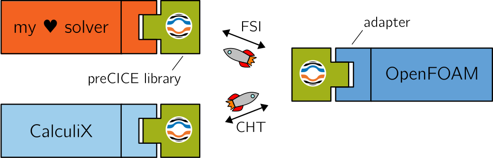
The adapter is defined in a *.xml file. Take the following example:
<?xml version="1.0" encoding="UTF-8" ?>
<precice-configuration>
  <log>
    <sink
      filter="%Severity% > debug and %Rank% = 0"
      format="---[precice] %ColorizedSeverity% %Message%"
      enabled="true" />
  </log>

  <data:vector name="Force" />
  <data:vector name="Displacement" />

  <mesh name="Fluid-Mesh" dimensions="2">
    <use-data name="Force" />
    <use-data name="Displacement" />
  </mesh>

  <mesh name="Solid-Mesh" dimensions="2">
    <use-data name="Displacement" />
    <use-data name="Force" />
  </mesh>

  <participant name="Fluid">
    <provide-mesh name="Fluid-Mesh" />
    <receive-mesh name="Solid-Mesh" from="Solid" />
    <read-data name="Displacement" mesh="Fluid-Mesh" />
    <write-data name="Force" mesh="Fluid-Mesh" />
    <mapping:rbf direction="read" from="Solid-Mesh" to="Fluid-Mesh" constraint="consistent">
      <basis-function:thin-plate-splines />
    </mapping:rbf>
    <mapping:rbf direction="write" from="Fluid-Mesh" to="Solid-Mesh" constraint="conservative">
      <basis-function:thin-plate-splines />
    </mapping:rbf>
  </participant>

  <participant name="Solid">
    <provide-mesh name="Solid-Mesh" />
    <read-data name="Force" mesh="Solid-Mesh" />
    <write-data name="Displacement" mesh="Solid-Mesh" />
    <watch-point mesh="Solid-Mesh" name="Flap-Tip" coordinate="0.25;0.0" />
    <export:vtk directory="precice-exports" />
  </participant>

  <m2n:sockets acceptor="Fluid" connector="Solid" exchange-directory=".." />

  <coupling-scheme:serial-explicit>
    <time-window-size value="2.5e-2" />
    <max-time value="2.5" />
    <participants first="Solid" second="Fluid" />
    <exchange data="Force" mesh="Solid-Mesh" from="Fluid" to="Solid" />
    <exchange data="Displacement" mesh="Solid-Mesh" from="Solid" to="Fluid" />
  </coupling-scheme:serial-explicit>
</precice-configuration>This file is for coupling a fluid and a solid solver together for a fluid-structure interaction simulation. On lines 10-11, we say that Force and Displacement are the variables we want to exchange. We then also define our different grids (lines 13-16 for the fluid mesh and lines 18-21 for our solid mesh), which have dimensions attached to them, as well as data that they should be using (which we specified before).
On lines 23-34, we create a fluid solver participant, where we state that we want to read in displacement data (line 26), and it should be applied to our fluid mesh. We also state here that force data should be extracted from this fluid mesh on line 27. We then specify how we want to map data from the solid to the fluid mesh, and vice versa, as shown on lines 28-33. We create a similar participant for the solid solver on lines 36-42.
Finally, we have to define our coupling scheme, which we do on lines 46-52. This is a rather simple example, but it shows you the basic working principle behind preCISE. The framework will now take and process this configuration file and make sure that the relevant fluid and structure solver will expose the required data, and it will map data from one mesh onto the other for each respective solver to consume.
TaskFlow, on the other hand, is slightly different. The name is actually quite good, in that TaskFlow provides us with a mechanism to specify different tasks and how they depend on each other. For example, take a 1-way fluid-structure simulation, where we first run the fluid solver to get forces, and then the solid solver to get displacements. Using a 1-way coupling scheme, this is all we do (opposed to a 2-way coupling scheme, where we also map displacements back to the fluid solver and then iterate over time on both solvers).
The following example code shows how a 1-way fluid structure interaction problem may be set up:
#include <taskflow/taskflow.hpp>
#include <fluid/solver.hpp>
#include <solid/solver.hpp>

int main() {

  tf::Executor executor;
  tf::Taskflow taskflow;

  FluidSolver fluid();
  SolidSolver solid();

  auto [fluidTask, solidTask] = taskflow.emplace(
    [] () { fluid.run(); },
    [] () { solid.run(); },
  );

  fluidTask.precede(solidTask);
  executor.run(taskflow).wait();

  return 0;
}You see, at its core, TaskFlow is just a sort of task scheduling application. We first have to import the TaskFlow header (which is a header-only library, convenient to get it started quickly without compilation needed). We then have to define a task and an executer object, which we do on lines 7-8. I also define here some dummy fluid and solid solver on lines 10-11, solely for demonstration purposes.
We then start to set up our tasks. On lines 13-16, we set up the fluidTask and solidTask, as well as defining what these tasks should be doing. In this simple example, we simply call the respective run() function on each solver, but we could place more complex C++ code here. On line 18, we say that the fluidTask has to run before the solidTask, and then we give the tasks to the executor, who will run the tasks for us.
So far, we haven't used any parallelism, but TaskFlow does integrate with parallelisation frameworks and thus provides support for parallelism between tasks. It provides higher-level functions (or flows, as they seem to be called) which take away some of the lower-level function calls. For example, the cudaFlow workflow provides functions for copying data to and from the CPU and GPU.
The power of TaskFlow is that you can define tasks (like the execution of one time step inside a fluid solver) as an abstract task (i.e. we don't care how it is achieved; that is the responsibility of the fluid solver), all we care about is how and when the task is executed, for example, after the solid solver has provided displacement information.
TaskFlow supports conditional task execution, which may be useful, for example, for checking the time at which the fluid solver is currently at, and then initiating data transfer (which itself is another task) between the fluid and the solid solver at particular points in time. If you want to get a more thorough introduction, have a look at their 2020 CppCon talk (ah, CppCon, another guilty pleasure of mine during lockdown ... I think I must have watched half of the conference):
Parallelisations for adaptive mesh refinement (AMR)
Adaptive mesh refinement itself is an area that is far from being a solved issue. At its core, adaptive mesh refinement allows us to refine a mesh in regions where we have large gradients (either through re-meshing or splitting of cells into smaller elements). The canonical example is shockwaves, and we probably want to resolve areas in which shockwaves occur. Another example may be the adaptive refinement of inflation layers, specifically the height of the first cell from the wall, though that is a much tougher problem to solve.
Sure, if I run a 2D airfoil example and I run some adaptive mesh refinement tutorials from the developers, I may be (mis)le(a)d to think that adaptive mesh refinement is easy, but it really isn't always that straightforward. The main issue, for me at least, is how we specify a criterion by which we select mesh cells that need to be adapted. For classic examples, like shockwaves, there may be good indicators we can use, for example, the gradient of the density field.
However, even if we do that, we still need to specify a threshold above which we want to refine a cell. So, what is a good value for the gradient above which we want to refine our cells? Keep in mind that the gradient itself is computed as the difference between two points divided by their distance. The distance is typically related to the cell size. Thus, the gradient is dependent on the cell size itself, and for varying cell sizes in our mesh, we get different gradient values across shock waves.
So, my question to you, again, is how we can define a value that will, ideally, only select cells in the region of shock waves and not anywhere else? This is a difficult task, at least if we want to generalise this for applications across various grids (and refinement criteria).
Or let's say we are interested in determining the separation point on an airfoil that hasn't stalled yet, but has a high angle of attack. A RANS model should be able to give us reasonably good predictions here, but we probably want to have good mesh refinement around the point of separation. What is a suitable criterion here? The local wall shear stresses are zero at the point of separation, so we may specify a band between positive and negative wall shear stresses in which we want to refine our mesh.
However, as we refine our mesh, the separation poitn may move, and so we have to dynamically coarsen and refine our mesh, which may be indeed feasible but either result in costly mesh refinement steps, or, an infinite loop in which we adapt/coarsen our mesh as a result of a moving separation point, which may or may not be due to the mesh refinement; we may simply pick up a transient behaviour. But how can we distinguish between a transient response and a response to our mesh refinement? We can't.
Another issue is the cell count explosion. If we are dealing with a 3D case, and, for the sake of argument, let's say that we use hexa elements in our mesh, each cell that is refined will be split into 8 cells. If we target 100,000 cells to be refined, then we have created 700,000 new cells (on top of the already 100,000 existing cells). If we don't have a good mechanism by which we can select only those cells we want to refine (which is difficult), we will end up with lots of additional cells.
A common solution to this problem is to limit the total number of new cells that can be created as part of the adaptive mesh refinement strategy, but how do we know that we have achieved sufficient refinement with this arbitrary cell limit? Well, in short, we don't, and so while we may believe that we have reduced uncertainties by refining cells in regions of strong gradients, all that we have done is trade one uncertainty for another.
Usually, uncertainties will decrease, and usually, results will improve, even if we have a sub-optimal adaptive mesh refinement strategy (i.e., a mechanism to select relevant cells to refine). But you wouldn't write a report saying, for example, that your lift coefficient should usually be expected to be around 0.425. CFD is full of uncertainties, and our job is to reduce uncertainties where we can, not introduce new ones.
The goal is not to produce colourful images, which is often the case when we get started with CFD (at that stage, it is fine; we need to start somewhere), but as we gain expertise, our goal shifts towards generating high-quality simulations, which require uncertainty management. Adaptive mesh refinement works against us, to some degree, on that front.
Now, let's bring this back to parallel computing. We may initially subdivide our mesh into N sub-domains. Each sub-domain is receiving an equal number of cells to work on. After some iterations, we may decide to refine our mesh, and after the first mesh adaptation is done, we will have, potentially, a wild difference between the number of cells on each sub-domain. This will then result in poor load balancing.
The solution to this problem is to dynamically adjust the number of cells per sub-domain, which results in better load balancing. However, this task is a costly one, and so any time we gain through improved parallel efficiency (i.e. by having a better load balance) must be offset by the time it takes to redistribute cells. In practice, we would set a tolerance for the load balance, after which repartition is required.
A good default value may be 10%, which states that we allow the number of cells between sub-domains to vary by 10% before redistributing cells across processors. And, as a side note, the same issue will occur not only during adaptive mesh refinement, but also during meshing in parallel in general. So, if we run our meshing algorithms in parallel, which, by definition, adaptively create new cells, the number of cells between sub-domains may quickly diverge and require a number of repartitioning steps.
In short, adaptive mesh refinement, or any other kind of dynamic mesh creation, will result in load balance issues, and load balancing is the number one reason that kills performance. It doesn't matter how much effort we put into making our code efficient. If we have poor load balancing, all of this effort is in vain. It is the same as buying a Ferrari for its speed, but then only driving it within the city. What's the point of the additional horse powers?
I presume showing-off is a large part of it, but I wouldn't know as a loyal Nissan customer (loyal as in my wife keeps making purchasing decisions that result in us buying Nissan cars, not as in I love the car or the brand; my car keeps falling apart in places I didn't even knew existed (but my mechanic is a very resourceful person when it comes to finding faults that need immediate replacement)).
My local Nissan dealer used to do the service for us and always bragged about their 100% original Nissan parts. But judging by how frequently they fail, I am much happier with 0% original Nissan parts. Anyways, given the recent news about Nissan's potential bankruptcy, this may be a future we all have to embrace.
Personally, I'll be using this as ammunition to convince my wife that it is time to upgrade from Japanese cars to Korean cars.
Update: We now own a Hyundai Sonata, but it was bought and registered in South Korea. I suppose it will be difficult to DLH it to the UK.
Note: I'm sure you came to this place to learn more about my car purchasing struggles. Life isn't just about CFD, it is also about Tom's first-world problems, well, at least this website is. Let's be honest, we are almost at the end of this article. How many people do you think will get this far into it?
Anyway, I seem to have lost my train of thought now (I wonder why), let's say we have finished adaptive mesh refinement, and move on to the next and final issue.
Issues in the age of exascale computing
Finally, let's talk about exascale computing. We have touched upon exascale computing in the introduction, that is, performing 10^18 floating point operations per second. When this large number of operations per second is involved, problems of a whole new scale start to emerge. But in order to understand this, let us look at an example.
According to the latest TOP500 list, ranking all of the registered high-performance computing (HPC) clusters in the world, the fastest cluster is El Capitan of Lawrence Livermore National Laboratory, featuring a peak performance of 1.8 ExaFLOPs across its 11,340,000 cores. Let's say we are granted access to the cluster, assuming full control over all 11,340,000 cores, and we are told we can do whatever we want with it.
So, naturally, we decided to run a direct numerical simulations (DNS), one of the persisting frontiers in CFD. Let's say we want to do something as benign as computing the lift and drag coefficient at a stall angle of attack. Surely, with 11,340,000, we ought to get some serious results. Well, we can do a simple back-of-the-envelope calculation to figure out what the largest Reynolds number is that we can simulate with this cluster.
To do that, we need to consider which length scales we want to resolve. On the larger end, we have some large characteristic lengthscale L, which could be the airfoil's chord or some measure of the domain size. On the smaller scale, we need to resolve the Kolmogorov length scale \eta, that is, the smallest turbulent length scale. So, we need a grid that has elements small enough to resolve \eta but which is, in dimension, large enough to capture L.
We can now use the definition and some typical scaling behaviours for our lengthscales. The Kolmogorov length scale is defined as:
\eta=\left(\frac{\nu^3}{\varepsilon}\right)^\frac{1}{4}
\tag{46}
Here, \nu is the kinematic viscosity, and \varepsilon is the dissipation. The dissipation itself scales well with the following correlation:
\varepsilon=\frac{U^3}{L}
\tag{47}
We want to express \eta in terms of a Reynolds number given as:
Re=\frac{UL}{\nu}\tag{48}To do that, we insert Eq.(47) into Eq.(46), which results in:
\eta=\left(\frac{\nu^3}{U^3/L}\right)^\frac{1}{4}=\left(\frac{\nu^3}{U^3L^{-1}}\right)^\frac{1}{4}=\frac{\nu^\frac{3}{4}}{U^\frac{3}{4}L^{-\frac{1}{4}}}\tag{49}We have L^{-\frac{1}{4}} in the denominator, and if we can bring this into the form of L^{\frac{3}{4}}, then we have the inverse definition of the Reynolds number, raised to the power of 3/4. In order to get this lengthscale, and remembering the exponent rule a^n\cdot a^m = a^{n+m}, we expand the fraction by L/L, which results in:
\eta=\frac{\nu^\frac{3}{4}}{U^\frac{3}{4}L^{-\frac{1}{4}}}\frac{L^\frac{4}{4}}{L^\frac{4}{4}}\tag{50}Now we combine the two length scales in the denominator and obtain:
L^{-\frac{1}{4}}\cdot L^\frac{4}{4}= L^{-\frac{1}{4}+\frac{4}{4}}=L^{\frac{3}{4}}\tag{51}Inserting this, we get:
\eta=\frac{\nu^\frac{3}{4}}{U^\frac{3}{4}L^{\frac{3}{4}}}L^\frac{4}{4} = L \frac{\nu^\frac{3}{4}}{U^\frac{3}{4}L^{\frac{3}{4}}} = L \left(\frac{\nu}{UL}\right)^\frac{3}{4} = \frac{L}{Re^\frac{3}{4}}=L\cdot Re^{-\frac{3}{4}}
\tag{52}
Now we know how \eta scales with the Reynolds number. We can make use of this definition by now computing how many grid points we need in one direction to resolve both the largest length scale L and the smallest length scale \eta. This is defined as:
N_\text{cells per direction}=\frac{L}{\eta}
\tag{53}
We know that we have to resolve \eta, so that is our smallest length scale. However, we also want to resolve L, and so we need to compute how many cells (of size \eta) fit inside our largest lengthscale L; hence, we divide \eta by L. And, if that is still not clear, for the sake of argument, let's say \eta=0.1mm, and L=1m, then, we need L/\eta=1/0.0001=10,000 cells in one direction to resolve both \eta and L at the same time.
So, in order to compute the number of cells per direction, we have to insert Eq.(\tag{52}) into Eq.(53). This results in:
N_\text{cells per direction}=\frac{L}{L}Re^\frac{3}{4} = Re^\frac{3}{4}\tag{54}This is for one direction, but in order to get the total number of cells, we need to multiply the number of points in all three coordinate directions, resulting in:
N_\text{total} = N_\text{cells per direction}^3 = \left(Re^\frac{3}{4}\right)^3=Re^\frac{9}{4}
\tag{55}
This number does not consider time stepping, but this is, as we will see in a second, also not really relevant here. It poses, in fact, a completely different problem that I'll return to. But let's finish off our example. Instead of assuming an arbitrary Reynolds number and then seeing how many grid points we can use, let's do it the other way around.
We know that El Capitan has 11,340,000 cores, and in our fictitious example, we were given all of them for our DNS. I also stated earlier that the best CFD solvers will scale well down to 50,000-100,000 cells per core. Taking a conservative pick, let's say that we want to run a DNS with 100,000 cells per core. We can now multiply that by our 11,340,000 cores and get a total mesh size of 1.134\cdot 10^{12} points, or 1.134 trillion points.
Well, it is 1.134 trillion points in English, but the Germans and French would say this is 1.134 billion points. This used to confuse me when I learned English; now I find the Germans irritating. Ah, well, no party is complete without the presence of at least one German and one French. They'll keep spirits high!
Let's go with 1.134\cdot 10^{12} grid points, which seems the least ambiguous. If that is the number of grid points that we can use, then we can compute the Reynolds number as:
Re=N_\text{total}^\frac{4}{9}=\left(1,.134\cdot 12^{12}\right)^\frac{4}{9}\approx 230,000 \approx 2\cdot 10^5\tag{56}This is laughable. Typical Reynolds numbers we achieve in aviation are around 10^6 to 10^7, and so even using the most potent super computer in the world, and assuming that we would be able to take over the entire system for our simulation, and that our code scales across the entire system without significant losses (all very strong assumptions), we would still fall one to two orders of magnitude short to simulate even a simple flow around an airfoil or wing, let alone an entire aircraft.
OK, so perhaps full aircraft simulations are not what we are after, but even with a modest number of cores, say, 100,000 cores for a single simulation, which is far more feasible, we would be able to get up to Reynolds numbers of about Re=30,000. This is, in realistic terms, what we can expect to be feasible with resources available in 2025. And this number is unlikely to change drastically in the near future, unless drastic changes to computer hardware are introduced (e.g. quantum computing).
OK, so let's say we settle for a modest Reynolds number of 30,000; being able to use 100,000 cores provides a whole new range of issues. For starters, let's think about domain decomposition. We now have to efficiently distribute the mesh across 100,000 cores. If we perform the domain decomposition step in parallel, then, well, we likely have a lot of communications between sub-domains just to check if we have a good distribution of cells (for load balancing).
Thus, our simulation may not even be the bottleneck; we may never get to it because the domain decomposition step just takes too long to finish.
I mentioned above that time stepping itself is also a problem. Why? As we saw in our simplified example for MPI, OpenMP, and CUDA, we really need to have lots of computations in parallel, and this only happens in space, that is, we can only parallelise computations in space across sub-domains, but not in time. We always compute one timestep after the other, which makes sense, but we could further enhance parallel efficiency if we could, somehow, parallelise our simulation in time as well.
Parallelisation in time is an ongoing research topic. At one point in my career, I saw it as a holy grail of parallel computing and devoted some time to learn about it, only to quickly realise that the limitations are likely too severe to ever overcome them for general-purpose CFD applications. There were good use cases for which parallelisation in time can be shown to yield good improvements, by not just parallelising the space loop but also the time loop, but these were, as far as I can tell, niche applications.
As far as I could tell, all applications used a simple model equation to demonstrate their effectiveness, but nothing was ever presented for the Navier-Stokes equations. Things may have changed, I may have missed a reference here or there, but the fact that parallelisation in time hasn't really been picked up as a mainstream research topic, despite its huge potential, probably is all you need to know about its true potential.
Don't get me wrong, if you feel like taking on the challenge and proving me wrong, I'd love for you to do that. I would be happy to accept that I am wrong if that means we get decent parallel-in-time performance for the Navier-Stokes equations.
Another issue that we also touched upon is the fact that compute nodes are physically distributed in space. As we increase the number of cores, we increase the physical distance between compute nodes and thus the time it takes for information to travel through the network. Thus, just having a large number of cores available doesn't mean we can utilise them efficiently; we will always lose some performance as we increase the number of cores, and some weak scaling analysis can highlight that.
Thus, the issues we face in parallel computing in the age of exascale computing are a lack of mature software solutions for large-scale parallel computations, a hardware bottleneck in terms of network transfer speeds, as well as pretty tough requirements in terms of strong scaling performance of our code, to ensure it scales well across thousands of processors.
Remember Amdahl's law? It tells us how good our parallelisation needs to be to get efficient scaling across thousands of processors, and writing general-purpose CFD codes that scale well across thousands of processors is a challenge no one person alone can likely master.
Summary
This has been yet another article that I planned to be much shorter, and then somehow exploded into this massive write-up that took about 2 months to finish. But I felt it was necessary to cover all aspects of parallel computing, including some code examples, to give you a flavour for how to deal with parallel computing, as well as to demonstrate some of its restrictions and bottlenecks.
In a nutshell, in an age in which processor speeds no longer double every 24 months according to Moore's law, but rather, the number of compute resources doubles every 24 months or so, we need to make use of code parallelisation in order to make use of the ever-increasing amount of computational power.
We saw that there are essentially two approaches available, which can be classified into shared memory and distributed memory approaches. In shared memory approaches, all cores have access to the same physical memory (RAM), and so all cores can simultaneously read and write data to memory. This makes parallelisation straightforward, and typically this approach is a good starting point when learning about parallel computations. OpenMP is the classic example of shared memory.
Distributed memory, on the other hand, assumes that each core gets its own private memory space that only it can read and write to and from. This means that if other cores need to have some data from surrounding processors, they have to send a request for data to be sent before they can use it. This approach means that it doesn't matter if the memory is located on the same physical memory (RAM) or somewhere else on a different compute node; data can always be sent via the network.
MPI is the typical example of a distributed memory approach and the de facto standard in parallel computing, at least for CFD applications. Another player on the block, CUDA, targeting NVIDIA GPUs for parallel computations, promises fast code execution, which typically performs much better than CPU-based parallelisation (often providing speed-ups an order of magnitude better than the same code parallelised for CPUs).
While CUDA has become the standard in Machine Learning applications, where the training and inference of any Machine Learning model without the use of CUDA seems impossible these days, CFD applications have not yet caught up to using GPUs as much, due to the sheer memory requirements we have in CFD. This typically means that our simulations are too big to fit on GPUs in the first place, and thus, we can't utilise the resources, unless we invest in some heavy-duty GPUs, which are orders of magnitude more expensive than a CPU with some decent RAM.
The parallelisation landscape is constantly changing, and what was the latest trend yesterday may as well be outdated tomorrow. One thing that seems to be standing strong in all of this, though, is MPI, and it is difficult to imagine a CFD future without a strong presence of MPI. Thus, if you want to become a proficient CFD coder, eventually you have to tackle MPI, which, as we have seen in the code examples I have provided, requires quite a bit of code manipulation to parallelise it.
One thing is for sure: parallelisation is such an important topic in CFD that without it, we can't be expected to do any serious CFD simulations, unless we are working on 1D research codes, for example, to improve methodologies. In that case, we may get away without using parallelisation of any form, but eventually, we need to face the music and learn MPI (or CUDA, or OpenMP), if we target to work in the field of CFD, specifically writing code, not necessarily just running simulations.
We have also come across some of the current challenges with parallelisations, such as how to parallelise multigrids, dealing with adaptive mesh refinement, and dealing with exascale computing, which introduces completely new compute scales that challenge existing hardware and software.
CFD is on an ever-evolving trajectory, and parallelisation is just one part of it. However, I believe that across the last articles in this series, I have given you a thorough overview of key concepts in CFD, along with challenges, and sometimes some fun little side projects, of which the STUPID turbulence model probably is my favourite.
It was developed on a hot summer day in South Korea (something like 45 degrees Celsius / 110 degrees Fahrenheit), without air conditioning and a neighbour playing about 3-4 notes on his guitar for about 6 hours. Perhaps you noticed the Korean influence on the model development ... What was torture back then, somehow survived as a fond memory.
In any case, this is the end for this series, but I have a few little fun projects planned for the near future, hopefully something for you to look forward to. Until then, I'll see you in the next article.

Tom-Robin Teschner is a senior lecturer in computational fluid dynamics and course director for the MSc in computational fluid dynamics and the MSc in aerospace computational engineering at Cranfield University.