How to discretise the Navier-Stokes equations

In our article on how to derive the Navier-Stokes equations from scratch, I showed you how we can derive the governing equations of fluid mechanics. Once we have found an equation that we want to solve, and we do not have an analytic solution available, we have to approximate a solution to that equation, for which we have three possible methods available to us: the finite difference method, the finite volume method, and the fine element method.

In this article, we will go through the motivation and rationale behind each discretisation method and I will show you that the finite volume method is just a generalised form of the finite difference method. We will see how to approximate the most common terms in fluid mechanics, and finish each discretisation section with the fully discretised Navier-Stokes equation for both an explicit and implicit time integration.

By the end of this article, you will have gained a deep understanding of how to discretise any partial differential equation. The equations that we will derive in this article can be implemented into a code and then solved numerically. Once you have understood this step, you will be able to derive and discretise your own equations without any issues. Let’s get started!

In this series

Introduction

Let’s take stock of what we have achieved thus far in this series. First, we derived the Navier-Stokes equations from start to end, and I showed you each step in the derivation, as well as which fundamental assumptions Navier, Stokes, and Saint-Venant made to arrive at this equation.

Then, we looked at how to classify any partial differential equation (PDE) into either a hyperbolic, parabolic, or elliptic equation. We saw that the character of this equation (or system of equations) will then determine what type or class of numerical schemes we ought to use to maximise accuracy and convergence rate.

Since there is no analytic solution available for the Navier-Stokes equations, we are left with having to approximate it. This brings us into the realm of numerical analysis, a subfield of mathematics, in which we replace symbolic manipulation of equations (as we have done thus far in this series) with efficient algorithms to approximate them.

Thus, the first step in the process of solving the Navier-Stokes equations is to discretise them into a discrete set of equations that can be used for a numerical approximation. There are three main types of discretisation that we use in numerical analysis, which are:

Finite difference method (FDM)
Finite volume method (FVM)
Finite element method (FEM)

The finite difference method approximates gradients directly. We find an equivalent expression that approximate first- and second-order derivatives, which we use to replace the symbolic derivatives in the Navier-Stokes equations. This is a quick and simple solution to a complex problem. However, across discontinuities (e.g. shock waves), gradients become infinitly large, and so a solution is difficult to obtain.

Most of the initial research on CFD, which began in ernest in the 1950s, was devoted to finding suitable numerical schemes that could treat the non-linear (advective) term in the Navier-Stokes equations. It was not until the 1980s that numerical schemes were introduced that could treat these non-linearities well (which we call high-resolution schemes these days).

The finite volume method makes use of the fact that we can rewrite a differential equation as an integral equation, i.e. we replace derivatives by integrals. Once we have an integral equation, solving discontinuities (shock waves) become not just a possibility but an integral part of the method. This makes this method a prime candidate for fluid mechanics application and it is the de facto standard for CFD applications.

Finally, we have the finite element method, where we have to rewrite our equations first into a weak formulation. Since we are now using a different set of equations, our goal is to find a solution to the weak form that approximates the original solution. I stated above that the finite volume method is the de facto standard in CFD; if you are living in Italy, you’ll likely find that the finite element method is the standard.

In this article, then, I want to look at each method and show how we can use them to discretise the Navier-Stokes equations. By the end of this article, you should be ablet o take your equations you want to solve and write them in an algebraic form. This form can now be solved using either an explicit or implicit time stepping method, which will be covered in the next article.

The finite difference method (FDM)

As stated above, the finite difference method approximates gradients directly. This approximaton is done through the Taylor series expansion, which provides us with a mechanism to replace symbolic derivatives with numeric approximations. Thus, once we undersand the Taylor series expansion, we can go straight to our Navier-Stokes equations, discretise, and solve them.

The Taylor series expansion

When I was a student and learning CFD for the first time, I inevitably came across the Taylor series expansion and wanted to know more. I followed a lecture where the professor opened the class with the words, “The Taylor series expansion is such a fundamental concept in numerical analysis that I don’t know what I would do without it. I use it every day” (or something to that effect, I am writing from memory here).

I have talked about the Taylor series expansion a few times already on this website, but it is wirth introducing it in the context of the finite difference method again to show its importance. We last looked at the Taylor series in the derivation of the navier-Stokes equation article, and I’ll reuse some of that material here and expand on it. If you feel comfortable with the Taylor series already, you can skip this section.

Whenever we are faced with a situation where we don’t know how a quantity is changing over time (or space), we use a Taylor series for that quantity, which will give us an approximation to an unknown function.

The idea is to replace the function we can’t solve analytically with a function that is easy to solve (at least numerically) and which approximates our original function, as long as we only approximate it within a small interval. If we can then easily calculate the derivatives of this new function, we have a winner.

To understand the small interval argument, say you want to forecast the temperature. Based on yesterday’s and today’s temperatures, you can probably make a reasonable assumption about tomorrow’s temperature. It won’t be exact, but it’ll get you close to it. If you consider the temperature in a week, a month, or even a year from now, your approximation won’t be as good, though, owing to the larger time interval.

Let’s work with this example. We want to forecast the temperature, but the only measurement we have available is today. What will be the temperature tomorrow? Well, if we only know today’s temperature, then we can just say it is going to be the same as today:

T(\mathrm{tomorrow})=T(\mathrm{today})

Obviously, this is going to be incorrect, but we will be closer, on average, than by making random guesses! Now, let’s introduce some terminology. Instead of writing $T(\mathrm{today})$ , we say that the temperature today (or right now) is given as $T(t)$ . Similarly, we write the temperature tomorrow to be $T(t+\Delta t)$ . Here, $\Delta t$ just means that we are looking some distance away from $t$ .

Thus, to express tomorrow, we can write $T(t+\Delta t)$ , the day after tomorrow would be $T(t+2\Delta t)$ , and we can also go in the other direction, i.e. yesterday would be $T(t-\Delta t)$ . Using this definition, we can rewrite the above equation as

T(t+\Delta t) = T(t)

Let’s say we keep continuing measuring the temperature, then we have data points available for several days. In our example above, we stated that we could also include the temperature from yesterday to make a better prediction:

T(t+\Delta t) = T(t) + \Delta t\frac{T(t) - T(t-\Delta t)}{\Delta t}

If you inspect the equation above, that is just the slope-intercept form of a straight line, i.e. $f(x)=b+mx$ , where we have $m=[T(t) - T(t-\Delta t)]\Delta t$ , $b=T(t)$ , and $x=t=\Delta t$ . If we look at our slope, then we can introduce the limit as

T(t+\Delta t) = T(t) + \Delta t\lim_{\Delta t\rightarrow 0}\frac{T(t) - T(t-\Delta t)}{\Delta t}=T(t)+\Delta t \frac{\mathrm{d}T}{\mathrm{d}t}

In other words, the slope is just the derivative. Since we have been collecting temperature data for days now, we can also compute higher order derivatives and introduce them into our equation by adding them to our expression for $T(t+\Delta t)$ :

T(t+\Delta t) = T(t)+\Delta t \frac{\mathrm{d}T}{\mathrm{d}t}+a \frac{\mathrm{d}^2T}{\mathrm{d}t^2}+b \frac{\mathrm{d}^3T}{\mathrm{d}t^3}+c \frac{\mathrm{d}^4T}{\mathrm{d}t^4}+d \frac{\mathrm{d}^5T}{\mathrm{d}t^5}+...+e \frac{\mathrm{d}^nT}{\mathrm{d}t^n}

Here, we have the unknowns $a, b, c, d, e$ , which need to be determined. Let’s consider what happens if we set $a=b=c=d=e=1$ . Assuming that we have a monotonically increasing temperature field (all derivatives are positive), each new derivative that we add to the predicted temperature of tomorrow will increase the temperature. With an infinite number of derivatives, we would then expect the temperature value to approach infinity itself.

Clearly, this is not a very good idea, so setting these coefficients to 1 will result in non-physical results. Instead, we want each derivative to have a diminishing influence over the predicted temperature $T(t+\Delta )$ . This is achieved, for example, in the following way:

T(t+\Delta t) = T(t)+\frac{\Delta t}{1!} \frac{\mathrm{d}T}{\mathrm{d}t}+\frac{\Delta t^2}{2!} \frac{\mathrm{d}^2T}{\mathrm{d}t^2}+\frac{\Delta t^3}{3!} \frac{\mathrm{d}^3T}{\mathrm{d}t^3}+\frac{\Delta t^4}{4!} \frac{\mathrm{d}^4T}{\mathrm{d}t^4}+\frac{\Delta t^5}{5!} \frac{\mathrm{d}^5T}{\mathrm{d}t^5}+...+\frac{\Delta t^n}{n!} \frac{\mathrm{d}^nT}{\mathrm{d}t^n}

While it would require some explaining to arrive at this expresson, for our intent and purposes, it is sufficient to accept that we have to introduce a weighting where the first derivative has the strongest weight, while each subsequent derivative will influence the predicted value of $T{t+\Delta t)$ less and less.

We can generalise the above expression for any quantity, and in fluid dynamics, such a generic quantity is tyically deonted by $\phi$ . The above expression thus becomes (only writing out the first derivatives now, but there are infinitly many, as expressed by the final term):

\phi(t+\Delta t) = \phi(t)+\frac{\Delta t}{1!} \frac{\mathrm{d}\phi}{\mathrm{d}t}+\frac{\Delta t^2}{2!} \frac{\mathrm{d}^2\phi}{\mathrm{d}t^2}+…+\frac{\Delta t^n}{n!} \frac{\mathrm{d}^n\phi}{\mathrm{d}t^n}

This is what is known as the Taylor series expansion. We can write it for approximation in space as well, where we have:

\phi(x+\Delta x) = \phi(x)+\frac{\Delta x}{1!} \frac{\mathrm{d}\phi}{\mathrm{d}x}+\frac{\Delta x^2}{2!} \frac{\mathrm{d}^2\phi}{\mathrm{d}x^2}+…+\frac{\Delta x^n}{n!} \frac{\mathrm{d}^n\phi}{\mathrm{d}x^n}

This is useful if we know some quantity in space at a location $x$ , and we want to know its value around the neighbourhood of $x$ . We can also reverse the Taylor series and predict value in the past:

\phi(t-\Delta t) = \phi(t)-\frac{\Delta t}{1!} \frac{\mathrm{d}\phi}{\mathrm{d}t}+\frac{\Delta t^2}{2!} \frac{\mathrm{d}^2\phi}{\mathrm{d}t^2}+…+(-1^n)\frac{\Delta t^n}{n!} \frac{\mathrm{d}^n\phi}{\mathrm{d}t^n}

Now, each odd derivative will be subtracted instead of added, as also shown by the last term. By analogy, we can translate this backward expansion in time to a space expansion as:

\phi(x-\Delta x) = \phi(x)-\frac{\Delta x}{1!} \frac{\mathrm{d}\phi}{\mathrm{d}x}+\frac{\Delta x^2}{2!} \frac{\mathrm{d}^2\phi}{\mathrm{d}x^2}+…+(-1^n)\frac{\Delta x^n}{n!} \frac{\mathrm{d}^n\phi}{\mathrm{d}x^n}

One thing to note here is that the Taylor series expansion shown above is exact, i.e., if we knew all derivatives (we may not have an infinite number!), then we could calculate the solution exactly. However, in practice, we typically only know one or two derivatives at best. We can still use the Taylor series expansion in this case, but we will be introducing an approximation that will have some influence down the line. We will look at this influence in a later article in this series.

If we want to consider, for example, only the first derivative and truncate the Taylor series expansion after this derivative, we use the following notation:

\phi(t+\Delta t) = \phi(t)+\frac{\Delta t}{1!} \frac{\mathrm{d}\phi}{\mathrm{d}t}+\mathcal{O}(\Delta t^2)

Here, the convention is to look at the first derivative that we have dropped from the Taylor series expansion (in this case, the second order derivative) and report its $\Delta$ value in parenthesis, i.e. $\mathcal{O}(\Delta t^2)$ . This turns out to be useful as the exponent of the $\Delta$ value directly corresponds with the order of approximation. In this case, we have $\mathcal{O}(\Delta t^2)$ and thus a second order approximation. The higher the order, the higher the potential accuracy of the solution.

So, what does that mean in practice? Let’s look at an example. Let’s assume we want to approximate the function $f(x)=e^x$ . Well, we know the exact solution (I just stated it), but if all we had were discrete points along this line, we could calculate derivatives numerically for this expression and then plot the overall solution as we introduce more and more derivatives. This is shown in the following animation, where $n$ is the number of derivatives that we are considering:

Approximating the function $f(x)=e^x$ with a Taylor series using an increasing number of terms that are retained in the series, indicated by the number $n$ . Image source

With eight derivatives, we do get a visually almost identical fit. However, now, consider we are at $x=0$ , and we set $\Delta x=0.01$ . For such a small interval, it is likely that even $n=1$ will result in a reasonable estimation, even if this Taylor series expansion would get inaccurate very quickly as $\Delta x$ is increased.

There is one additional aspect which is not evident from the above animation. The animation is done for a smooth function, i.e. $f(x)=e^x$ . But once you add just a small amount of noise, your higher-order derivatives will start to oscillate, and your fit will be pretty bad. Since numerical data is always contaminated with some degree of noise through round-off errors, modelling errors, and other sources of uncertainties, you have to strike a balance between accuracy and stability.

Linking the Taylor series expansion to a computational mesh

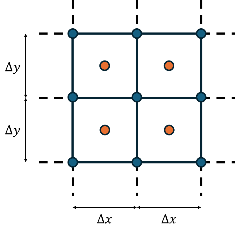
We looked at the general Taylor series expansion above, what I want to do in this section is to show you how we can link that to a computational mesh. Consider the figure of a 2D mesh shown below:

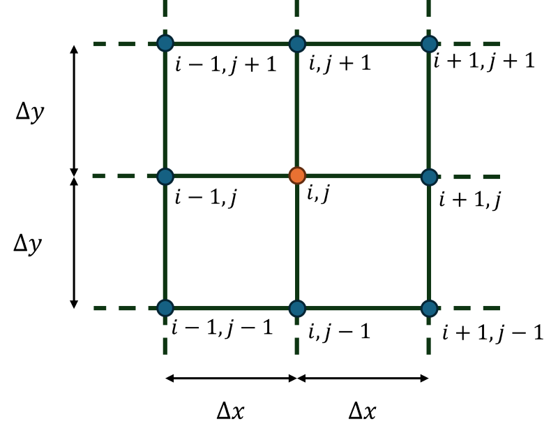
When we discretise our Navier-Stokes equations, we want to solve it at each grid point. That is, we are seeking the solution for the velocity and pressure (at a minimum), potentially also the density and temperature, along with other quantities. Let’s say that we are currently located at the grid point in the center, highlighted in orange.

In this case, we have a regular Cartesian grid. We can see that each cell has the same width and height $\Delta x$ and $\Delta y$ , respectively. If we want to obtain information from one of the surrounding grid points, we need to be able to index them.

In 2D, we introduce an $i, j$ indexing, where the index $i$ runs along the x-axis, and $j$ runs along the y-axis. In 3D, we would extend this to $i,j,k$ . Thus, if we look at our Taylor series expansion and we see a notation like $\phi(x)$ and $\phi(x+\Delta x$ , we can replace that with $\phi_i$ and $\phi_{i+1}$ . This is the notation you will most commonly find in textbooks.

In 2D, we simply extend this idea and introduce the $j$ index as well. So for example, if we had $\phi(x+\Delta x, y-\Delta y$ , then this would translate to $\phi_{i+1,j-1}$ . But what if we are considering a 2D grid and we are now performing a Taylor series expansion in time? Well, let’s have a look at the figure below:

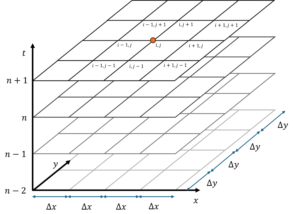
Here, we see that we have to introduce a third axis in time for our 2D Cartesian grid. We can now have solutions for each grid point at different time levels, which are usually labelled with the letter $n$ . The current time level $t$ is thus labelled as $n$ , while a Taylor series expansion in time, i.e. $t+\Delta t$ is labelled as $n+1$ .

We use a slightly different convention, though, when it comes to Taylor series expansions in time. If we are considering expansions in space, then we use subscripts and the letters $i, j$ as seen before. In time, however, we use superscripts, which allows us to treat expansions in time and space simultaneously. Thus, $\phi(x, y, t+\Delta t)$ becomes $\phi_{i,j}^{n+1}$ . We will use this notation throughout the rest of this section.

Approximating first-order derivatives

Let’s then turn our attention to the approximation of first-order derivatives. Writing out the Taylor series exapnsion in time, using a second-order approximation, results in the following:

\phi(t+\Delta t) = \phi(t) + \frac{\mathrm{d} \phi}{\mathrm{d} t}\frac{\Delta t}{1!} + \mathcal{O}(\Delta t^2)

Our goal is to solve this equation now for the first-order derivative. Thus, we isolate that on the right-hand side as:

\frac{\phi(t+\Delta t) - \phi(t)}{\Delta t} = \frac{\mathrm{d} \phi}{\mathrm{d} t} + \mathcal{O}(\Delta t)

Hang on, why did the order drop from second to first? When we divide by $\Delta t$ , we have to divide all terms in the Taylor series expansion, and this will reduce the order of the first derivative that we are no longer considering. To see this more clearly, consider the third-order accurate expansion:

\phi(t+\Delta t) = \phi(t) + \frac{\mathrm{d} \phi}{\mathrm{d} t}\frac{\Delta t}{1!} + \frac{\mathrm{d} \phi^2}{\mathrm{d} t^2}\frac{\Delta t^2}{2!} + \mathcal{O}(\Delta t^3)

If we divide this expression now by $\Delta t$ , we arrive at the following expression:

\frac{\phi(t+\Delta t)}{\Delta t} = \frac{\phi(t)}{\Delta t} + \frac{\mathrm{d} \phi}{\mathrm{d} t} + \frac{\mathrm{d} \phi^2}{\mathrm{d} t}\frac{\Delta t}{2!} + \mathcal{O}(\Delta t^2)

If we now truncate the Taylor series expansion after the first derivative, we get

\frac{\phi(t+\Delta t)}{\Delta t} = \frac{\phi(t)}{\Delta t} + \frac{\mathrm{d} \phi}{\mathrm{d} t} + \mathcal{O}(\Delta t)

Thus, with the understanding that this approximation is only going to be first-order accurate at best, we can drop the $\mathcal{O}(\Delta t)$ term from the equation and write:

\frac{\mathrm{d} \phi}{\mathrm{d} t} \approx \frac{\phi(t+\Delta t) - \phi(t)}{\Delta t}=\frac{\phi^{n+1}-\phi^n}{\Delta t}

Similarly, we can find the first order derivative in space as:

\frac{\mathrm{d} \phi}{\mathrm{d} x} \approx \frac{\phi(x+\Delta x) - \phi(x)}{\Delta x}=\frac{\phi_{i+1}-\phi_i}{\Delta x}

Using a backward Taylor series expansion, we can find the following approximation in space and time as:

\frac{\mathrm{d} \phi}{\mathrm{d} t} \approx \frac{\phi(t) - \phi(t-\Delta t)}{\Delta t}=\frac{\phi^n-\phi^{n-1}}{\Delta t}

\frac{\mathrm{d} \phi}{\mathrm{d} x} \approx \frac{\phi(x) - \phi(x-\Delta x)}{\Delta x}=\frac{\phi_i-\phi_{i-1}}{\Delta x}

This first order approximation really is a curse and a blessing in disguise. It is a blessing, as it is a very stable scheme. If you throw a discontinous signal at it (i.e. a shock wave), it handles that with ease, i.e. it does not introduce any oscillatory behaviour near discontinuities. It is a curse at te same time, as this stability comes at the cost of a lot of numerical diffusion.

Numerical diffusion will apply excessive diffusion to your solution. Gradients won’t be preserved as sharply as they perhaps are, and thus, we gain stability but at the cost of losing physical information. This process is similar to downscaling an image. Reducing the resolution means the picture won’t be as sharp as before, and if we zoom in, sharp edges will appear smoother now.

To overcome this, much attention in the early days of CFD research was devoted to developing second-order accurate schemes. We can produce such as scheme with relative ease by considering two Taylor series expansions as:

\phi(t+\Delta t) = \phi(t) + \frac{\mathrm{d} \phi}{\mathrm{d} t}\frac{\Delta t}{1!} + \frac{\mathrm{d} \phi^2}{\mathrm{d} t^2}\frac{\Delta t^2}{2!} + \mathcal{O}(\Delta t^3)

The second expansion is done backwards in time as:

\phi(t-\Delta t) = \phi(t) - \frac{\mathrm{d} \phi}{\mathrm{d} t}\frac{\Delta t}{1!} + \frac{\mathrm{d} \phi^2}{\mathrm{d} t^2}\frac{\Delta t^2}{2!} + \mathcal{O}(\Delta t^3)

We subtract the second (backwards) Taylor series expansion from the first (forward) to arrive at:

\phi(t+\Delta t) - \phi(t-\Delta t)= 2\frac{\mathrm{d} \phi}{\mathrm{d} t}\frac{\Delta t}{1!} + \mathcal{O}(\Delta t^3)

Isolating the derivative results in:

\frac{\mathrm{d} \phi}{\mathrm{d} t}=\frac{\phi(t+\Delta t) - \phi(t-\Delta t)}{2\Delta t} + \mathcal{O}(\Delta t^2)

With the understanding that this approximation is second-order accurate, we may write this derivative in time and space as:

\frac{\mathrm{d} \phi}{\mathrm{d} t}\approx\frac{\phi(t+\Delta t) - \phi(t-\Delta t)}{2\Delta t}=\frac{\phi^{n+1}-\phi^{n-1}}{2\Delta t}

\frac{\mathrm{d} \phi}{\mathrm{d} x}\approx\frac{\phi(x+\Delta x) - \phi(x-\Delta x)}{2\Delta x}=\frac{\phi_{i+1}-\phi_{i-1}}{2\Delta x}

Approximating second-order derivatives

Approximating second-order derivatives follows a similar logic with a slight complication. Let’s consider the fourth-order accurate Taylor series expansion in time (forward):

\phi(t+\Delta t) = \phi(t)+\frac{\Delta t}{1!} \frac{\mathrm{d}\phi}{\mathrm{d}t}+\frac{\Delta t^2}{2!} \frac{\mathrm{d}^2\phi}{\mathrm{d}t^2}+\frac{\Delta t^3}{3!} \frac{\mathrm{d}^3\phi}{\mathrm{d}t^3}+\mathcal{O}(\Delta t^4)

If we were to solve this now for the second order derivative, we would still be left with an expression for the first-order derivative. If we know that value, great, we could insert it, but we can use a little trick to get rid of it. For this, consider the fourth-order accurate Taylor series expansion in time, this time backwards:

\phi(t-\Delta t) = \phi(t)-\frac{\Delta t}{1!} \frac{\mathrm{d}\phi}{\mathrm{d}t}+\frac{\Delta t^2}{2!} \frac{\mathrm{d}^2\phi}{\mathrm{d}t^2}-\frac{\Delta t^3}{3!} \frac{\mathrm{d}^3\phi}{\mathrm{d}t^3}+\mathcal{O}(\Delta t^4)

Since we have the first-order derivative in both equations but with an opposite sign, we can add both equations together, which will result in the first derivative being dropped (we used the same trick above to construct the second-order accurate first-order derivative). The same is true for the third-order derivative, which will drop for the same reasons. This results in:

\phi(t+\Delta t) + \phi(t-\Delta t) = 2\phi(t)+\Delta t^2 \frac{\mathrm{d}^2\phi}{\mathrm{d}t^2}+\mathcal{O}(\Delta t^4)

We can solve this expression now for the second-order derivative again to arrive at the following expression in time:

\frac{\phi(t+\Delta t) - 2\phi(t) + \phi(t-\Delta t) }{\Delta t^2}=\frac{\mathrm{d}^2\phi}{\mathrm{d}t^2}+\mathcal{O}(\Delta t^2)

The order of approximation dropped to second now, as we had to divide by $\Delta t^2$ . With this understanding at hand, we can write the approximation for the second-order derivative as:

\frac{\mathrm{d}^2\phi}{\mathrm{d}t^2}\approx \frac{\phi(t+\Delta t) - 2\phi(t) + \phi(t-\Delta t) }{\Delta t^2}=\frac{\phi^{n+1}-2\phi^n+\phi^{n-1}}{\Delta t^2}

In a similar manner, we can approximate the second-order derivative in space as:

\frac{\mathrm{d}^2\phi}{\mathrm{d}x^2}\approx \frac{\phi(x+\Delta x) - 2\phi(x) + \phi(x-\Delta x) }{\Delta x^2}=\frac{\phi_{i+1}-2\phi_i+\phi_{i-1}}{\Delta x^2}

Pros and Cons of the finite difference method

Well, we have found a pretty good way to discretise derivatives, haven’t we? Why would we ever want to use something different? Well, let’s put it this way, the finite difference method is still in use, but only in academic research codes, really. I am not aware of any commercial solver that is using the finite difference method. Let’s have a look at what the pros and cons are of the finite difference method.

Pros

Well, it is dead simple to use, period! If you need to solve a partial differential equation, just throw a few approximations of the first-order and second-order derivatives, and you’ll have a solution in no time.
We looked at the Taylor series expansion, and one nice thing about it is that the more terms we include in our approxiation, the higher the order of our approximation will be. Constructing higher-order approximation requires a bit more background reading, but it is something we can easily achieve once we know how. This makes the finite difference method a very lucrative method for turbulence modelling research, especially direct numerical simulations (DNS).

Cons

Its biggest advantage is also its biggest disadvantage: We approximate derivatives with the finite difference method. In fluid dynamics, we may be interested in resolving discontinuities (shock waves, interfaces between two phases (air-water), etc.). The derivative across a discontinuity is undefined, thus limiting the application of the finite difference method to smooth solutions (though schemes have been proposed that can work with discontinuous signals).
The finite difference approximation is limited to be used with structured grids. It can’t work with unstructured grids because the derivatives require the $i,j$ indexing we saw before. If we can’t index our neighbours, then we can’t find approximations to our derivatives. This is the biggest limitation of the method, and as a result, it is less commonly used these days.
If we want to extend the finite difference method beyond Cartesian coordinates, we need to introduce curvelinear coordinates, which require a coordinate transformation. This will add a lot of additional terms to our equation, making it easier to introduce programing errors and in general, increasing complexity. We have not looked at this coordinate transformation, but if you are curious, the books of Anderson and Hoffmann and Chiang (Vol.1) have an excellent discussion of the topic.

The discretised Navier-Stokes equations

In order to discretise the Navier-Stokes equation, we really need to be talking about numerical schemes first. This will be an entire article in its own right in this series, so I won’t go into any depth here. Suffice it to say that the non-linear term in the Navier-Stokes equations requires special treatment, which we will gloss over in this section. Once we talk about numerical schemes, we’ll pick this up again.

Secondly, we will also talk about explicit and implicit methods in a separate article, so I won’t elaborate on this aspect here either. However, I want to provide the full discretised equations here for reference. In a nutshell, in explicit discretisations, all derivatives are calculated at time level $n$ , while implicit discretisations are evaluated at $n+1$ , requiring a linear system of equation solver to obtain a solution. We looked at how to write our own linear solver library some time ago, which I link here for reference.

We’ll look at the incompressible form of the Navier-Stokes equation; the compressible form is derived analogously.

Explicit formulation

Continuity equation

The continuity equation is given as:

\nabla\cdot\mathbf{u}=0

In 2D Cartesian coordinates, this equation can be written in scalar form as:

\frac{\partial u}{\partial x}+\frac{\partial v}{\partial y}=0

This can be approximated using a second-order approximation for both derivatives

\frac{u_{i+1,j}^n -u_{i-1,j}^n}{2\Delta x}+\frac{v_{i,j+1}^n -v_{i,j-1}^n}{2\Delta y}=0

Momentum equation

The incompressible momentum equation without any source terms can be written as:

\frac{\partial \mathbf{u}}{\partial t} + (\mathbf{u}\cdot\nabla)\mathbf{u} = -\frac{1}{\rho}\nabla p + \nu\nabla^2\mathbf{u}

First, we have to write this equation again in scalar form. If we do that, we obtain two equations: one in the x-direction and one in the y-direction.

\frac{\partial u}{\partial t}+u\frac{\partial u}{\partial x}+v\frac{\partial u}{\partial y}=-\frac{1}{\rho}\frac{\partial p}{\partial x}+\nu\frac{\partial^2 u}{\partial x^2}+\nu\frac{\partial^2 u}{\partial y^2}

\frac{\partial v}{\partial t}+u\frac{\partial v}{\partial x}+v\frac{\partial v}{\partial y}=-\frac{1}{\rho}\frac{\partial p}{\partial y}+\nu\frac{\partial^2 v}{\partial x^2}+\nu\frac{\partial^2 v}{\partial y^2}

These two scalar equations can now be approximated using a first-order approximation in time and for the non-linear terms while using a second-order accurate approximation for the pressure and the diffusive term.

\frac{u_{i,j}^{n+1}-u_{i,j}^n}{\Delta t}+u_{i,j}^n\frac{u_{i,j}^n-u_{i-1,j}^n}{\Delta x}+v_{i,j}^{n}\frac{u_{i,j}^{n}-u_{i,j-1}^{n}}{\Delta y}=-\frac{1}{\rho}\frac{p_{i+1,j}^{n}-p_{i-1,j}^{n}}{2\Delta x}+\nu\frac{u_{i+1,j}^{n}-2u_{i,j}^{n}+u_{i-1,j}^{n}}{\Delta x^2}+\nu\frac{u_{i,j+1}^{n}-2u_{i,j}^{n}+u_{i,j-1}^{n}}{\Delta y^2}

\frac{v_{i,j}^{n+1}-v_{i,j}^n}{\Delta t}+u_{i,j}^n\frac{v_{i,j}^n-v_{i-1,j}^n}{\Delta x}+v_{i,j}^{n}\frac{v_{i,j}^{n}-v_{i,j-1}^{n}}{\Delta y}=-\frac{1}{\rho}\frac{p_{i,j+1}^{n}-p_{i,j-1}^{n}}{2\Delta y}+\nu\frac{v_{i+1,j}^{n}-2v_{i,j}^{n}+v_{i-1,j}^{n}}{\Delta x^2}+\nu\frac{v_{i,j+1}^{n}-2v_{i,j}^{n}+v_{i,j-1}^{n}}{\Delta y^2}

Implicit formulation

Continuity equation

The continuity equation is now solved at the time level $n+1$ , which is in line with an implicit formulation. This results in:

\frac{u_{i+1,j}^{n+1} -u_{i-1,j}^{n+1} }{2\Delta x}+\frac{v_{i,j+1}^{n+1} -v_{i,j-1}^{n+1} }{2\Delta y}=0

Momentum equation

In a similar manner, the implicit formulation of the momentum equation becomes:

\frac{u_{i,j}^{n+1}-u_{i,j}^n}{\Delta t}+u_{i,j}^n\frac{u_{i,j}^{n+1}-u_{i-1,j}^{n+1}}{\Delta x}+v_{i,j}^{n}\frac{u_{i,j}^{n+1}-u_{i,j-1}^{n+1}}{\Delta y}=-\frac{1}{\rho}\frac{p_{i+1,j}^{n}-p_{i-1,j}^{n}}{2\Delta x}+\nu\frac{u_{i+1,j}^{n+1}-2u_{i,j}^{n+1}+u_{i-1,j}^{n+1}}{\Delta x^2}+\nu\frac{u_{i,j+1}^{n+1}-2u_{i,j}^{n+1}+u_{i,j-1}^{n+1}}{\Delta y^2}

\frac{v_{i,j}^{n+1}-v_{i,j}^n}{\Delta t}+u_{i,j}^n\frac{v_{i,j}^{n+1}-v_{i-1,j}^{n+1}}{\Delta x}+v_{i,j}^{n}\frac{v_{i,j}^{n+1}-v_{i,j-1}^{n+1}}{\Delta y}=-\frac{1}{\rho}\frac{p_{i,j+1}^{n}-p_{i,j-1}^{n}}{2\Delta y}+\nu\frac{v_{i+1,j}^{n+1}-2v_{i,j}^{n+1}+v_{i-1,j}^{n+1}}{\Delta x^2}+\nu\frac{v_{i,j+1}^{n+1}-2v_{i,j}^{n+1}+v_{i,j-1}^{n+1}}{\Delta y^2}

There are two things to notice here:

First, the time derivatives of the non-linear term are evaluated at time level $n+1$ . However, the coefficients, or velocity components in front of the derivatives, are evaluated at time level $n$ . This is known as linearisation and is required, as our linear solvers can only deal with, well, linear systems. There are ways to extend this to non-linear systems as well, but this is very much a research effort and very time-consuming. The linearisation shown above is very common.
Second, the pressure derivative is evaluated at time level $n$ as well. This is required as each equation can only be solved for one quantity. The above equations are solved for $u$ and $v$ , respectively, thus, the pressure has to be solved for at time level $n$ .

In the article on implicit time integration methods, I’ll show you how the above equations are solved.

The finite volume method

In this section, we will look at the finite volume discretisation and see how we can use that to approximate our governing equations. The easiest way to do that is by considering the following generic 1D transport equation:

\frac{\partial \phi}{\partial t}+a\frac{\partial \phi}{\partial x}=b\frac{\partial^2 \phi}{\partial x^2}

We do that because it contains all essential terms (time, first-order, and second-order derivatives). If we understand how to discretise this equation, then we can apply the same knowledge to our Navier-Stokes equations. By comparing it to the above equation, we see that only the pressure derivative term is missing.

The idea of the finite volume method can be summarised as follows: Each flow is contained within its boundaries. For a flow around an airfoil, for example, we have farfield boundaries. For a flow within a pipe, we have the physical walls that mark the boundary of the flow. Our goal is to find an approximate solution to the Navier-Stokes equations within this domain. To do so, we discretise it with a finite number of small volumes (elements), that combined will fill the entire domain.

These finite volumes are then connected at their faces and this will be used to make up our computational grid. What I have just described could have also been summarised as follows: We need to find a computational grid for our domain, and the cells that are generated will be our finite volumes. There is a difference, though, in the way we treat the grid compared to the finite difference method discussed above.

In the finite volume method, we don’t approximate the solution at the vertices of the cells. Since each cell (volume) is supposed to represent the solution, we need to find the solution within each volume. Thus, we introduce a centroid, which you can think of as the geometric center of the cell itself. We store all information (velocity, pressure, temperature, etc.) at this centroid, and then we assume that this value does not change across the cell (volume). This is shown below, where the centroid is now shown in orange.

So, if we want the value to be constant at the centroid and fill the entire space of the volume, what do we do? We integrate over the volume! This is exactly what the finite volume method is doing. Let’s see how we can achieve that.

So, returning to our generic 1D transport equation, let’s start applying the volume integrals. First things first, we have to do this integration for each cell (volume). So in the figure above, if that was our computational domain, we would have to write the volume integration for each of these four cells.

However, the good news is that we perform the integration only once, and then apply that integrated equation to each cell. In addition, since we are dealing with an unsteady equation, i.e. we have a time derivative as well, we also need to integrate our equation over time. This is to track how our equation is changing in time between two time levels, i.e. between $t$ and $t+\Delta t$ .

Let’s do that and apply this to our generic transport equation:

\int_t^{t+\Delta t}\int_V\frac{\partial \phi}{\partial t}\mathrm{d}V\mathrm{d}t+a\int_t^{t+\Delta t}\int_V\frac{\partial \phi}{\partial x}\mathrm{d}V\mathrm{d}t=b\int_t^{t+\Delta t}\int_V \frac{\partial^2 \phi}{\partial x^2}\mathrm{d}V\mathrm{d}t

Here, we have treated $a$ and $b$ as constants so they can be taken outside the derivatives. The next thing is to evaluate each integral. We’ll do this separately for each derivative and then see how to solve the entire equation later when we bring all of this together again into a single equation.

Approximating first-order temporal derivatives

Let’s start with the time derivative. We can always change the order of integration, which we will do here first. Then, our time derivative becomes:

\int_V\int_t^{t+\Delta t}\frac{\partial \phi}{\partial t}\mathrm{d}t\mathrm{d}V

From calculus, we know that the integral of a derivative is just the underlying function itself, i.e. $\int f'(x)\mathrm{d}t=f(x)$ . Thus, the time derivative vanishes, but we have to evaluate the integral at the respective bounds. Assuming that the change in time is slow (i.e. we have a time step that is sufficiently small), we can write the following:

\int_V\phi\Big|_t^{t+\Delta t} \mathrm{d}V=\int_V[\phi(t+\Delta t)-\phi(t)] \mathrm{d}V=\int_V (\phi^{n+1}-\phi^n) \mathrm{d}V

Now, we simply integrate over the volume to arrive at:

\int_V (\phi^{n+1}-\phi^n) \mathrm{d}V=(\phi^{n+1}-\phi^n)V

Thus, whenever we are faced with a time derivative, we can approximate it using the following relationship:

\int_V\int_t^{t+\Delta t}\frac{\partial \phi}{\partial t}\mathrm{d}t\mathrm{d}V=(\phi^{n+1}-\phi^n)V

Approximating first-order spatial derivatives

First-order spatial derivatives work a bit differently to time derivatives. There is a trick we can (and will) do, which will change our derivative approximation. There is a very specific reason why we want to employ this trick, yet you won’t find any textbook explaining it to you! You have to bring enough of your own curiosity and willingness to go through some math textbooks to eventually be presented with an explanation. I’ll shortcut this for you today so you have more time for tik tok later, you are welcome!

Let’s look at the spatial, first-order derivative again:

a\int_t^{t+\Delta t}\int_V\frac{\partial \phi}{\partial x}\mathrm{d}V\mathrm{d}t

Before we go on to integrate in time, as we did with the time derivative term, let’s turn to our little trick. Open any textbook on CFD, explaining the finite volume method. Once they have reached this point in the derivation, you will hear something to the effect of: and now we use the Gauss theorem to transform our volume integral into a surface integral. Ok, let’s do this first, and then we will discuss it:

a\int_t^{t+\Delta t}\int_An\cdot\phi\,\mathrm{d}A\mathrm{d}t

Let’s focus on this transformation. According to the Gauss theorem, we can replace any volume integral with a surface integral using the following relationship:

\int_V\frac{\partial\phi}{\partial x}\mathrm{d}V=\int_An\cdot\phi\,\mathrm{d}A

Here, $n$ is the normal vector. This is stating, in plain English, that instead of watching how a quantity is changing over time, we simply watch how it is changing across its boundaries. Still not clear? I don’t blame you, I am giving you text book definitions which are really unhelpful to grasp this. Let’s take an example, which will hopefully make it more clear.

Say you want to measure the volume of a balloon. How would you do that? Sure, you can do a volume integral if you know the shape analytically, but we probably don’t have an equation that exactly describes the balloon, so doing a volume integral will be rather difficult. Here is our trick: Instead of measuring the volume, why don’t we measure the massflow rate going into the balloon?

If we know the density $\rho$ of the fluid going into our balloon, we know the mass flow rate $\dot{m}$ , and we know for how long we are filling the balloon (total time $T$ ), we can come up with a pretty good estimate of the overall volume by computing it from the aforementioned quantities as

V=\frac{\dot{m}T}{\rho}

From dimensional grounds, we have

\frac{\left[\frac{kg}{s}\right][s]}{\left[\frac{kg}{m^3}\right]}=\frac{kg\cdot s\cdot m^3}{kg\cdot s}=m^3

which is, well, a volume. So this checks out. Surely, this is an easier way to compute the overall volume of the balloon. And this is how the Gauss theorem works.

OK, great, we have now somewhat of an intuition of why this works, but why bother? It turns out that calculating the volume integral is no more challenging than the surface integral, at least in CFD terms. Well, the surface integral formulation provides a hidden advantage for us that is not immediately evident. But before we can see that, we need to finish the finite volume method discretisation first.

We saw that one of the side effects of the Gauss theorem is that we lose the derivative, so we can’t integrate the equation in the same way in time as we did for the time derivative. Instead, we simply carry out the integration:

a\int_t^{t+\Delta t}\int_An\cdot\phi\,\mathrm{d}A\mathrm{d}t=a\int_An\cdot\phi\,\mathrm{d}A\Big|_t^{t+\Delta t}=a\Delta t\int_An\cdot\phi\,\mathrm{d}A

The time integral bounds will be eventually evaluated as $(\Delta t + t) - t$ , so only the time step $\Delta t$ remains. Since it does not change during the integration, we can put it in front of the integral together with a constant $a$ .

Now, we need to face the surface derivative. Before, we were able to simply integrate over the volume, which resulted in the volume itself being multiplied by our quantity of interest. In this case, we first have to define the surfaces. Let’s return to the finite volume approximation we saw before:

Each cell in this example has 4 faces that connect itself to another cell (or, well, volume). So instead of checking how our quantity of interest is changing within the cell (volume), we check how much of our quantity of interest is going in or out through the faces (this is equivalent to looking at how much mass flow is going into our balloon).

So, to do so, we replace the area integral with a summation, where we now go over each face within a cell and check how much of our quantity is going in or out of our cell:

a\Delta t\int_An\cdot\phi\,\mathrm{d}A\approx a\Delta t\sum_{i=1}^{n_{faces}}n_f\cdot \phi_i A_i

There are a few observations we can do here:

The normal vector has changed to the normal vector of the face, and it will point out of the cell .
$\phi_i$ is the interpolated value between two centroids to the corresponding face. The interpolation algorithm will play a crucial role in getting the value of $\phi_i$ accurately predicted at the face.
We multiply each $\phi_i$ by the area of that face. In 2D, Cartesian coordinates, the area of the faces will be either $\Delta x$ or $\Delta y$ .

Let’s say that we have a 1D flow on the following grid:

If we are at point $i$ , i.e. the cell at the center, then we could write our approximation as:

a\Delta t\sum_{i=1}^{n_{faces}}n_f\cdot \phi_i A_i=a\Delta t(\phi_{f_2}A_{f_2}-\phi_{f_1}A_{f_1})

The question becomes how we approximate $\phi_{f_2}$ and $\phi_{f_1}$ . A naive approach would be the following:

\phi_{f_2}=\frac{1}{2}\left(\phi_i+\phi_{i+1}\right)

and

\phi_{f_1}=\frac{1}{2}\left(\phi_i+\phi_{i-1}\right)

This is known as the central scheme. It turns out that the central scheme is one of the worst approximations we can do, but we go with it for the moment as it makes it easier to work with our equation and then explore in a later article how to make a better approximation here. Inserting this into our equation above, we arrive at:

a\Delta t(\phi_{f_2}A_{f_2}-\phi_{f_1}A_{f_1})=\frac{a\Delta t}{2}[\left(\phi_i+\phi_{i+1}\right)A_{f_2}-\left(\phi_i+\phi_{i-1}\right)A_{f_1}]

Here, I have taken the constant $1/2$ out of the brackets.

To summarise, a first order spatial derivative can be approximated in general as:

a\int_t^{t+\Delta t}\int_V\frac{\partial \phi}{\partial x}\mathrm{d}V\mathrm{d}t\approx a\Delta t\sum_{i=1}^{n_{faces}}n_f\cdot \phi_i A_i

After we have taken an educated guess as to how to approximate the values of $\phi$ at the faces, in this case, a central scheme, we may further expand the above equation to the following form:

a\int_t^{t+\Delta t}\int_V\frac{\partial \phi}{\partial x}\mathrm{d}V\mathrm{d}t\approx \frac{a\Delta t}{2}[\left(\phi_i+\phi_{i+1}\right)A_{f_2}-\left(\phi_i+\phi_{i-1}\right)A_{f_1}]

Why is the Gauss theorem king?

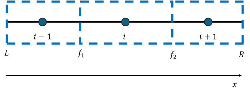
So, let’s have a final look then at why we bother with the Gauss theorem and what its use is. Let’s consider our 1D flow again:

We only have 3 cells to make life easy, and I have labelled all faces. We want to approximate the first-order derivative here. Let’s start with the cell on the left, i.e. with the centroid at $i-1$ . Ignoring the

a\Delta t\sum_{i=1}^{n_{faces}}n_f\cdot \phi_i A_i=a\Delta t(\phi_{f_1}A_{f_1}-\phi_LA_L)

When we are at face $f_1$ , the normal vector is pointing along the positive x-direction, hence the product $\phi_{f_1}A_{f_1}$ is positive. When we are at face $f_2$ , however, the normal vector points against the x-direction (remember we specified that the normal vector always points out of the cell). Thus, the product $\phi_L A_L$ is negative. As a result, we don’t see the normal vector anymore.

Let’s write out the approximation for the second and third volumes as well. We get:

a\Delta t\sum_{i=1}^{n_{faces}}n_f\cdot \phi_i A_i=a\Delta t(\phi_{f_2}A_{f_2}-\phi_{f_1}A_{f_1})

and

a\Delta t\sum_{i=1}^{n_{faces}}n_f\cdot \phi_i A_i=a\Delta t(\phi_{R}A_{R}-\phi_{f_2}A_{f_2})

Since this is a 1D example, the area of the faces will be the same for all. Well, in 1D, it isn’t defined, but that isn’t an issue. Since we assume it to be the same in the entire domain, we can cancel it out of our equations. Similarly, if we assume $a\Delta t$ to be constant and to be the same for all terms, then we can cancel them from our approximations. If we do that, then we are left with the following equations:

Cell 1 ( $i-1$ )

\phi_{f_1}-\phi_L

Cell 2 ( $i$ )

\phi_{f_2}-\phi_{f_1}

Cell 3 ( $i+1$

\phi_R-\phi_{f_2}

Rather simple, right? Let’s see what happens when we add the solution for all cells together. In the end, this is what we would do (not exactly in the form shown below; it is a bit more convoluted, but the simplistic addition adopted here is representative of what would happen in a real solver):

(\phi_{f_1}-\phi_L)+(\phi_{f_2}-\phi_{f_1})+(\phi_R-\phi_{f_2})

Let’s re-arrange this into the following form:

\phi_L + \phi_R + \underbrace{\phi_{f_1} - \phi_{f_1}}_{=0} + \underbrace{\phi_{f_2} - \phi_{f_2}}_{=0}=\phi_L + \phi_R

This is known as a telescoping series. But why is it important? Well, after we have made all of our approximations to the derivatives, the only things left are the values of $\phi$ at the left and right boundaries, i.e. the values we put into our system as externally imposed values. All internally approximated values will cancel each other out, thus conserving whatever $\phi$ represents.

If $\phi$ stands for density, then we have conservation of mass, if it is density times velocity, we have conservation of momentum, if it is temperature, we have conservation of energy, and so on. Using the Gauss theorem aligns well with our conservation laws (the Navier-Stokes equations) of fluid mechanics.

Approximating second-order spatial derivatives

Thankfully, second-order spatial derivatives are not too dissimilar to first-order spatial derivatives and we can carry over a lot from what we have just learned. Let’s look at the second order derivative case again; we had:

b\int_t^{t+\Delta t}\int_V \frac{\partial^2 \phi}{\partial x^2}\mathrm{d}V\mathrm{d}t

The first thing we’ll do is split the derivative into two first order derivatives so that we can bring the above form into something we can recognise from the first-order derivative case. We get:

b\int_t^{t+\Delta t}\int_V \frac{\partial^2 \phi}{\partial x^2}\mathrm{d}V\mathrm{d}t=b\int_t^{t+\Delta t}\int_V \frac{\partial}{\partial x}\frac{\partial \phi}{\partial x}\mathrm{d}V\mathrm{d}t

We can now apply everything we saw above, which will result in:

b\int_t^{t+\Delta t}\int_V \frac{\partial}{\partial x}\frac{\partial \phi}{\partial x}\mathrm{d}V\mathrm{d}t\approx b\Delta t\sum_{i=1}^{n_{faces}}n_f\cdot \frac{\partial \phi_i}{\partial x} A_i

We are now faced with the issue of having to evaluate the derivative as part of our approximation. Let’s see how we would go about that. Returning to the 1D example that we saw before:

If we are currently in the second cell at $i$ , we could approximate the derivative to the right as:

\frac{\partial \phi_{f_2}}{\partial x}\approx \frac{\phi_{i+1}-\phi_{i}}{\Delta x}

And, to the left, we can approximate the derivative as:

\frac{\partial \phi_{f_1}}{\partial x}\approx \frac{\phi_{i}-\phi_{i-1}}{\Delta x}

With these definitions in hand, we can insert them into our discretised equations. For example, for the second cell (at $i$ ), we would have

b\int_t^{t+\Delta t}\int_V \frac{\partial^2 \phi}{\partial x^2}\mathrm{d}V\mathrm{d}t\approx b\Delta t\left( \frac{\phi_{i+1}-\phi_{i}}{\Delta x}A_{f_2}-\frac{\phi_{i}-\phi_{i-1}}{\Delta x}A_{f_1} \right)

Bringing it all together: the discretised generic transport equation

Let us now put all the approximations of the generic transport equation into a single equation and then further simplify the expression. As a reminder, this is the equation we started with:

\frac{\partial \phi}{\partial t}+a\frac{\partial \phi}{\partial x}=b\frac{\partial^2 \phi}{\partial x^2}

Inserting now the various approximations for the time and spatial derivatives, we obtain the following equation:

\underbrace{(\phi^{n+1}-\phi^n)V}_{\partial \phi/\partial t}+\underbrace{\frac{a\Delta t}{2}[\left(\phi_i+\phi_{i+1}\right)A_{f_2}-\left(\phi_i+\phi_{i-1}\right)A_{f_1}]}_{a(\partial \phi/\partial x)} = \underbrace{b\Delta t\left( \frac{\phi_{i+1}-\phi_{i}}{\Delta x}A_{f_2}-\frac{\phi_{i}-\phi_{i-1}}{\Delta x}A_{f_1} \right)}_{b(\partial^2 \phi/\partial x^2)}

I have taken the approximate versions here, where we used the central scheme in the first-order derivative, as well as the discretised derivative in the second-order term. Let’s start to simplify this equation by first dividing this equation by the time step. This results in:

\frac{\phi^{n+1}-\phi^n}{\Delta t}V+\frac{a}{2}[\left(\phi_i+\phi_{i+1}\right)A_{f_2}-\left(\phi_i+\phi_{i-1}\right)A_{f_1}] = b\left( \frac{\phi_{i+1}-\phi_{i}}{\Delta x}A_{f_2}-\frac{\phi_{i}-\phi_{i-1}}{\Delta x}A_{f_1} \right)

Next, consider our starting point for the discretisation again:

If we have a two-dimensional case, then we can say that our faces on each side of a cell have an area of $\Delta x$ or $\Delta y$ . From dimensional grounds, this does not make sense, so the common practice is to say that we multiply this area by a unit length (1 meter) in the third direction, which we are not resolving. This gives us units of $m^2$ , but it doesn’t change the value of the area itself.

So if the areas are either $\Delta x$ or $\Delta y$ , then the volume of each cell can be expressed as $V=\Delta x\Delta y$ . Thus, if we divide an area by the volume, i.e. $A/V$ , we would get either $A/V=1/\Delta x$ or $1/\Delta y$ .

So if we apply that to our (simplified) 1D example, dividing the equation by the volume results in:

\frac{\phi^{n+1}-\phi^n}{\Delta t}+\frac{a}{2\Delta x}[\left(\phi_i+\phi_{i+1}\right)-\left(\phi_i+\phi_{i-1}\right)] = b\left( \frac{\phi_{i+1}-\phi_{i}}{\Delta x^2}-\frac{\phi_{i}-\phi_{i-1}}{\Delta x^2} \right)

At this point, let us reformulate the above expression slightly. We can rewrite the equation in the following form:

\frac{\phi^{n+1}-\phi^n}{\Delta t}+a\frac{\phi_{i+1}-\phi_{i-1}}{2\Delta x} = b\frac{\phi_{i+1}-2\phi_{i}+\phi_{i-1}}{\Delta x^2}

If we have a quick look into the finite difference method section, we can see that our aproximations to the derivatives are equivalent to our finite difference method approximations. This is a good thing, this means that our finite difference method and finite volume method are consistent.

I should also say, though, that they are only equivalent for Cartesian grids, which is what we have considere here. If we go to unstructured grids, as we have discussed, there is no expression for the finite difference method. So, the finite volume method is a generalisation and extension of the finite difference method.

At this point, we need to make a decision about the time level we want to approximate our unknowns $\phi$ at, i.e. do we want to approximate them at the time level $n$ or at time level $n+1$ ? The former will result in an explicit discretisation, while the latter will lead to an implicit discretisation.

Typically, we want to use an implicit discretisation. While it is a bit more challenging to solve (we need a linear system of equation solvers), doing so will bring more advantages than disadvantages. So, let’s go ahead and start with an implicit treatment first. We will later see that we can easily transform that into an explicit treatment as well.

We start by writing the respective time levels at our quantity of interest $\phi$

\frac{\phi^{n+1}_i-\phi^n_i}{\Delta t}+a\frac{\phi_{i+1}^{n+1}-\phi_{i-1}^{n+1}}{2\Delta x} = b\frac{\phi_{i+1}^{n+1}-2\phi_{i}^{n+1}+\phi_{i-1}^{n+1}}{\Delta x^2}

Next, we want to group the equations into known and unknown quantities. Everything that is unknown goes on the left side, and everything that is known will go on the right side.

\phi^{n+1}_i\frac{1}{\Delta t}+a\frac{\phi_{i+1}^{n+1}-\phi_{i-1}^{n+1}}{2\Delta x} - b\frac{\phi_{i+1}^{n+1}-2\phi_{i}^{n+1}+\phi_{i-1}^{n+1}}{\Delta x^2} = \phi_i^{n}\frac{1}{\Delta t}

We want to express everything in terms of our unknowns. Thus, we rewrite our equations in a form that factors out $\phi$ from the fractions. This results in:

\phi_i^{n+1}\left(\frac{1}{\Delta t}+\frac{2}{\Delta x^2}\right)+\phi_{i-1}^{n+1}\left(-\frac{a}{2\Delta x}-\frac{b}{\Delta x^2}\right)+\phi_{i+1}^{n+1}\left(\frac{a}{2\Delta x}-\frac{b}{\Delta x^2}\right)= \phi_i^{n}\left(\frac{1}{\Delta t}\right)

The convention now is that we abbreviate the equation above by introducing the following coefficients:

a_i=\left(\frac{1}{\Delta t}+\frac{2}{\Delta x^2}\right)\\a_{i-1}=\left(-\frac{a}{2\Delta x}-\frac{b}{\Delta x^2}\right)\\a_{i+1}=\left(\frac{a}{2\Delta x}-\frac{b}{\Delta x^2}\right)\\b=\phi_i^{n}\left(\frac{1}{\Delta t}\right)

With this definition in place, we can now write our equation in the following form:

\phi_i^{n+1}a_i+\phi_{i-1}^{n+1}a_{i-1}+\phi_{i+1}^{n+1}a_{i+1}= b

This is now the discretised form for a single cell (volume). If we wanted to write this out for all cells, we would end up with a matrix of the following form:

\begin{bmatrix}a_i & a_{i+1} & 0 & 0 & \dots & 0\\a_{i-1} & a_i & a_{i+1} & 0 & & 0\\0 & a_{i-1} & a_i & a_{i+1} & & 0\\ \vdots & & & & \ddots & \\0 & & & & a_{i-1} & a_i \end{bmatrix}\begin{bmatrix}\phi_1^{n+1}\\\phi_2^{n+1}\\\phi_3^{n+1}\\\vdots\\\phi_n^{n+1}\end{bmatrix}=\begin{bmatrix}b_1\\b_2\\b_3\\ \vdots\\b_n\end{bmatrix}

This can also be written as

\mathbf{Ax}=\mathbf{b}

To find a solution to the above system of linear equations, we have to invert the matrix $\mathbf{A}$ . This is expensive, as the matrix will contain as many rows and columns as we have cells in our mesh. Thus, we’d rather find an approximation which can be calculated much quicker but requires an iterative solution procedure.

I did write about these issues at length in the series on linear system of equation solvers. We looked at how to efficiently store matrices, as well as how to solve them iteratively using the conjugat gradient method. I’ve also shown how to put this together and solve the 1D heat diffusion equation using the finite volume method as discussed above. If you want to see how all of the above is used in practice, then this series is for you.

So this is it, really. You now have all the tools you need to discretise an equation with the finite volume method. I just want to make one last comment before looking at the pros and cons of the finite volume method. For this, let’s inspect the implicit discretised form of the equation again:

\phi_i^{n+1}a_i+\phi_{i-1}^{n+1}a_{i-1}+\phi_{i+1}^{n+1}a_{i+1}= b

If we wanted to express this now as an explicit discretisation instead, we simply change the time levels for the unknowns at $i\pm 1$ . Then, we get:

\phi_i^{n+1}a_i= b

Here, we have now $b$ defined as:

b=\phi^n_i\left(\frac{1}{\Delta t}\right)-\phi_{i-1}^{n}a_{i-1}-\phi_{i+1}^{n}a_{i+1}

Since we have a single unknown ( $\phi_i^{n+1}$ ) in this equation, we can solve it directly without the need for a linear system solver.

Pros and Cons of the finite volume method

So, we have spend some time now deriving he finite volume method for various derivatives, let’s have a look at what some advantages and disadvantages are, before we write out the entire discretisation for the Navier-Stokes equation.

Pros

The finite volume method, together with the Gauss theorem, have in-built conservation properties, which make them incredibly reliable as an approximation procedure for CFD applications.
The finite volume method is mainly conserned with fluxes going across faces (Gauss theorem, what goes in and out of a cell). Since we have a face-based discretisation, it doesn’t matter what underlying structure our cells have. Thus, the finite volume method is inherently suitable to be used with unstructured grids.

Cons

We have lost the nice and clean representation of derivatives compared to the finite difference method. Thus, implementing the finite volume method is somewhat more challenging.
Being able to use unstructured grids means we no longer have access to an arbitrary number of neighbour nodes/cells. Thus, we can only ever know our direct neighbour cells, which makes the finite volume method, at best, second-order accurate. Extensions to higher orders exist, but the devil is in the details. Anyone can derive a higher-order numerical scheme, but that will not make the approximation necessarily better than second-order. If you are interested in higher-order accuracy, use the finite difference method, or, if you need unstructured grids, the finite element method, but that comes with its own array of issues

The discretised Navier-Stokes equations

At last, let us have a look at the discretised Navier-Stokes equations and see how the finite volume method looks like in practice. Similar to the finite difference method, we will consider the incompressible version of the Navier-Stokes equations. We will discretise them with the understanding that they can’t be solved in the form that I show here, for that, we first need to talk about pressure-velocity coupling algorithms for incompressible flows. This will be another article in this series.

Explicit formulation

Continuity equation

The continuity equation is again given as:

\nabla\cdot\mathbf{u}=0

Integrating this equation over a finite volume and applying the Gauss theorem results in:

\int_V\nabla\cdot\mathbf{u}\,\mathrm{d}V=\int_A n\cdot\mathbf{u}_f\,\mathrm{d}A\approx\sum_{i=1}^{n_{faces}}n\cdot\mathbf{u}_iA_i

In 2D Cartesian coordinates, this equation will now be approximated on the following cell arrangement:

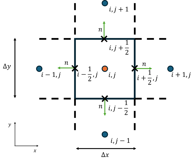
Let’s look at the summation in detail. We have to go over all faces. Thus, if we take the face to the east (at $i+\frac{1}{2},j$ ), we have the following contribution in the summation:

n_{i+\frac{1}{2},j}\cdot\mathbf{u}_{i+\frac{1}{2},j}A_{i+\frac{1}{2},j}=\begin{bmatrix}1\\0\end{bmatrix}\cdot\begin{bmatrix}u_{i+\frac{1}{2},j}\\v_{i+\frac{1}{2},j}\end{bmatrix}\Delta y=u_{i+\frac{1}{2},j}\Delta y

In a similar manner, we can find the contribution at the west face (at $i-\frac{1}{2},j$ )

n_{i-\frac{1}{2},j}\cdot\mathbf{u}_{i-\frac{1}{2},j}A_{i-\frac{1}{2},j}=\begin{bmatrix}-1\\0\end{bmatrix}\cdot\begin{bmatrix}u_{i-\frac{1}{2},j}\\v_{i-\frac{1}{2},j}\end{bmatrix}\Delta y=-u_{i-\frac{1}{2},j}\Delta y

In the north and south direction, we have, respectively:

n_{i,j+\frac{1}{2}}\cdot\mathbf{u}_{i,j+\frac{1}{2}}A_{i,j+\frac{1}{2}}=\begin{bmatrix}0\\1\end{bmatrix}\cdot\begin{bmatrix}u_{i,j+\frac{1}{2}}\\v_{i,j+\frac{1}{2}}\end{bmatrix}\Delta x=v_{i,j+\frac{1}{2}}\Delta x

n_{i,j-\frac{1}{2}}\cdot\mathbf{u}_{i,j-\frac{1}{2}}A_{i,j-\frac{1}{2}}=\begin{bmatrix}0\\-1\end{bmatrix}\cdot\begin{bmatrix}u_{i,j-\frac{1}{2}}\\v_{i,j-\frac{1}{2}}\end{bmatrix}\Delta x=-v_{i,j-\frac{1}{2}}\Delta x

Putting this all together and assuming now an explicit time integration, we arrive at:

\int_V\nabla\cdot\mathbf{u}^n\,\mathrm{d}V=\int_A n\cdot\mathbf{u}^n_f\,\mathrm{d}A\approx\sum_{i=1}^{n_{faces}}n\cdot\mathbf{u}^n_iA_i=u^n_{i+\frac{1}{2},j}\Delta y-u^n_{i-\frac{1}{2},j}\Delta y+v^n_{i, j+\frac{1}{2}}\Delta x - v^n_{i,j-\frac{1}{2}}\Delta x =0

This can be shortend to:

(u^n_{i+\frac{1}{2},j}-u^n_{i-\frac{1}{2},j})\Delta y+(v^n_{i, j+\frac{1}{2}} - v^n_{i,j-\frac{1}{2}})\Delta x =0

Momentum equation

The incompressible momentum equation without any source terms can be written as (using $\mathbf{I}$ as the identity matrix):

\frac{\partial \mathbf{u}}{\partial t} + (\mathbf{u}\cdot\nabla)\mathbf{u} = -\frac{1}{\rho}\nabla p\mathbf{I} + \nu\nabla^2\mathbf{u}

Applying our finite volume approximations by integrating each term over the volume and time results in (I have introduced the superscript $n$ here to show that we are solving the equation now with an explicit scheme):

\int_t^{t+\Delta t}\int_V\frac{\partial \mathbf{u}}{\partial t}\,\mathrm{d}V\mathrm{d}t + \int_t^{t+\Delta t}\int_V(\mathbf{u}^n\cdot\nabla)\mathbf{u}^n\,\mathrm{d}V\mathrm{d}t = \int_t^{t+\Delta t}\frac{1}{\rho}\int_V\nabla p^n\mathbf{I}\,\mathrm{d}V\mathrm{d}t + \int_t^{t+\Delta t}\nu\int_V\nabla^2\mathbf{u}^n\,\mathrm{d}V\mathrm{d}t

We can apply the time integration as we have done above for the generic transport equation to arrive at

(\mathbf{u}^{n+1}-\mathbf{u}^{n})V+\Delta t\int_V(\mathbf{u}^n\cdot\nabla)\mathbf{u}^n\,\mathrm{d}V=\frac{\Delta t}{\rho}\int_V\nabla p^n\mathbf{I}\,\mathrm{d}V+\nu\Delta t\int_V\nabla^2\mathbf{u}^n\,\mathrm{d}V

Applying the Gauss theorem to it, we arrive at:

(\mathbf{u}^{n+1}-\mathbf{u}^{n})V+\Delta t\int_A(\mathbf{u}^n\cdot n)\mathbf{u}^n\,\mathrm{d}A=\frac{\Delta t}{\rho}\int_An\cdot p^n\mathbf{I}\,\mathrm{d}A+\nu\Delta t\int_A\nabla\mathbf{u}^n\,\mathrm{d}A

Now we replace the integrals with summations:

(\mathbf{u}^{n+1}-\mathbf{u}^{n})V+\Delta t\sum_{i=1}^{n_{faces}}(\mathbf{u}_i^n\cdot n_i)\mathbf{u}_i^nA_i=\frac{\Delta t}{\rho}\sum_{i=1}^{n_{faces}}n_i\cdot p^n_i\mathbf{I}A_i+\nu\Delta t\sum_{i=1}^{n_{faces}}\nabla\mathbf{u}^n_iA_i

Now, we write the scalar equations for both the x and y direction. We start with the x direction and obtain:

(u^{n+1}_{i,j}-u^{n}_{i,j})V_{i,j} + \Delta t(u^{n}_{i+\frac{1}{2},j}u^{n}_{i+\frac{1}{2},j}A_{i+\frac{1}{2},j}-u^{n}_{i-\frac{1}{2},j}u^{n}_{i-\frac{1}{2},j}A_{i-\frac{1}{2},j}) + \Delta t(v^{n}_{i,j+\frac{1}{2}}u^{n}_{i,j+\frac{1}{2}}A_{i,j+\frac{1}{2}}-v^{n}_{i,j-\frac{1}{2}}u^{n}_{i,j-\frac{1}{2}}A_{i,j-\frac{1}{2}}) = \\ \Delta t(p^n_{i+\frac{1}{2},j}A_{i+\frac{1}{2},j}-p^n_{i-\frac{1}{2},j} A_{i-\frac{1}{2},j}) + \nu\Delta t\left(\frac{\partial u}{\partial x}\Big|^n_{i+\frac{1}{2},j}A_{i+\frac{1}{2},j}-\frac{\partial u}{\partial x}\Big|^n_{i-\frac{1}{2},j}A_{i-\frac{1}{2},j}\right) + \nu\Delta t\left(\frac{\partial u}{\partial y}\Big|^n_{i,j+\frac{1}{2}}A_{i,j+\frac{1}{2}}-\frac{\partial u}{\partial y}\Big|^n_{i,j-\frac{1}{2}}A_{i,j-\frac{1}{2}}\right)

At this point, let us simplify the equation before we continue. We do that by inserting the following expressions:

A_{i+\frac{1}{2},j}=A_{i-\frac{1}{2},j}=\Delta y\\A_{i,j+\frac{1}{2}}=A_{i,j-\frac{1}{2}}=\Delta x

This results in:

(u^{n+1}_{i,j}-u^{n}_{i,j})V_{i,j} + \Delta t\Delta y(u^{n}_{i+\frac{1}{2},j}u^{n}_{i+\frac{1}{2},j}-u^{n}_{i-\frac{1}{2},j}u^{n}_{i-\frac{1}{2},j}) + \Delta t\Delta x(v^{n}_{i,j+\frac{1}{2}}u^{n}_{i,j+\frac{1}{2}}-v^{n}_{i,j-\frac{1}{2}}u^{n}_{i,j-\frac{1}{2}}) = \\ \Delta t\Delta y(p^n_{i+\frac{1}{2},j}-p^n_{i-\frac{1}{2},j}) + \nu\Delta t\Delta y\left(\frac{\partial u}{\partial x}\Big|^n_{i+\frac{1}{2},j}-\frac{\partial u}{\partial x}\Big|^n_{i-\frac{1}{2},j}\right) + \nu\Delta t\Delta x\left(\frac{\partial u}{\partial y}\Big|^n_{i,j+\frac{1}{2}}-\frac{\partial u}{\partial y}\Big|^n_{i,j-\frac{1}{2}}\right)

We can now further simplify this equation by dividing by the timestep $\Delta t$ , as well as the volume $V$ , noting that the volume for a 2D Cartesian grid is calculated as $V=\Delta x\Delta y$ . This results in:

\frac{u^{n+1}_{i,j}-u^{n}_{i,j}}{\Delta t} + \frac{1}{\Delta x}(u^{n}_{i+\frac{1}{2},j}u^{n}_{i+\frac{1}{2},j}-u^{n}_{i-\frac{1}{2},j}u^{n}_{i-\frac{1}{2},j}) + \frac{1}{\Delta y}(v^{n}_{i,j+\frac{1}{2}}u^{n}_{i,j+\frac{1}{2}}-v^{n}_{i,j-\frac{1}{2}}u^{n}_{i,j-\frac{1}{2}}) = \\ \frac{1}{\Delta x}(p^n_{i+\frac{1}{2},j}-p^n_{i-\frac{1}{2},j}) + \frac{\nu}{\Delta x}\left(\frac{\partial u}{\partial x}\Big|^n_{i+\frac{1}{2},j}-\frac{\partial u}{\partial x}\Big|^n_{i-\frac{1}{2},j}\right) + \frac{\nu}{\Delta y}\left(\frac{\partial u}{\partial y}\Big|^n_{i,j+\frac{1}{2}}-\frac{\partial u}{\partial y}\Big|^n_{i,j-\frac{1}{2}}\right)

Even though we said that central differencing is perhaps not the best approach, we do that here to bring our equation into a discretised form that we can solve. We will discuss in another article which better options exist. The central differencing scheme can be expressed as:

\phi_{i+\frac{1}{2},j}=0.5(\phi_{i,j}+\phi_{i+1,j}) \\ \phi_{i-\frac{1}{2},j}=0.5(\phi_{i,j}+\phi_{i-1,j}) \\ \phi_{i,j+\frac{1}{2}}=0.5(\phi_{i,j}+\phi_{i,j+1}) \\ \phi_{i,j-\frac{1}{2}}=0.5(\phi_{i,j}+\phi_{i,j-1})

For the derivatives, we can use the following approximation, which works well in practice (and is commonly done):

\frac{\partial \phi}{\partial x}\Big|^n_{i+\frac{1}{2},j}=\frac{\phi_{i+1,j}-\phi_{i,j}}{\Delta x}\qquad\qquad\frac{\partial \phi}{\partial y}\Big|^n_{i+\frac{1}{2},j}=\frac{\phi_{i+1,j}-\phi_{i,j}}{\Delta y} \\ \frac{\partial \phi}{\partial x}\Big|^n_{i-\frac{1}{2},j}=\frac{\phi_{i,j}-\phi_{i-1,j}}{\Delta x}\qquad\qquad\frac{\partial \phi}{\partial y}\Big|^n_{i-\frac{1}{2},j}=\frac{\phi_{i,j}-\phi_{i-1,j}}{\Delta y} \\ \frac{\partial \phi}{\partial x}\Big|^n_{i,j+\frac{1}{2}}=\frac{\phi_{i,j+1}-\phi_{i,j}}{\Delta x}\qquad\qquad\frac{\partial \phi}{\partial y}\Big|^n_{i,j+\frac{1}{2}}=\frac{\phi_{i,j+1}-\phi_{i,j}}{\Delta y} \\ \frac{\partial \phi}{\partial x}\Big|^n_{i,j-\frac{1}{2}}=\frac{\phi_{i,j}-\phi_{i,j-1}}{\Delta x}\qquad\qquad\frac{\partial \phi}{\partial y}\Big|^n_{i,j-\frac{1}{2}}=\frac{\phi_{i,j}-\phi_{i,j-1}}{\Delta y} \\

Inserting these definitions results in:

\frac{u^{n+1}_{i,j}-u^{n}_{i,j}}{\Delta t} + \frac{1}{2\Delta x}[u^{n}_{i+\frac{1}{2},j}(u^n_{i,j}+u^n_{i+1,j})-u^{n}_{i-\frac{1}{2},j}(u^n_{i,j}+u^n_{i-1,j})] + \frac{1}{2\Delta y}[v^{n}_{i,j+\frac{1}{2}}(u^n_{i,j}+u^n_{i,j+1})-v^{n}_{i,j-\frac{1}{2}}(u^n_{i,j}+u^n_{i,j-1})] = \\ \frac{1}{2\Delta x}[(p^n_{i,j}+p^n_{i+1,j})-(p^n_{i,j}+p^n_{i-1,j})] + \frac{\nu}{\Delta x}\left(\frac{u^n_{i+1,j}-u^n_{i,j}}{\Delta x}-\frac{u^n_{i,j}-u^n_{i-1,j}}{\Delta x}\right) + \frac{\nu}{\Delta y}\left(\frac{u^n_{i,j+1}-u^n_{i,j}}{\Delta y}-\frac{u^n_{i,j}-u^n_{i,j-1}}{\Delta y}\right)

We can simplify the pressure and diffusive term further, which results in:

\frac{u^{n+1}_{i,j}-u^{n}_{i,j}}{\Delta t} + \frac{1}{2\Delta x}[u^{n}_{i+\frac{1}{2},j}(u^n_{i,j}+u^n_{i+1,j})-u^{n}_{i-\frac{1}{2},j}(u^n_{i,j}+u^n_{i-1,j})] + \frac{1}{2\Delta y}[v^{n}_{i,j+\frac{1}{2}}(u^n_{i,j}+u^n_{i,j+1})-v^{n}_{i,j-\frac{1}{2}}(u^n_{i,j}+u^n_{i,j-1})] = \\ \frac{p^n_{i+1,j}-p^n_{i-1,j}}{2\Delta x} + \nu\frac{u^n_{i+1,j}-2u^n_{i,j}+u^n_{i-1,j}}{\Delta x^2}+ \nu\frac{u^n_{i,j+1}-2u^n_{i,j}+u^n_{i,j-1}}{\Delta y^2}

We can now factorise the velocity components. We will collect them on the left-hand side for the moment. This step results in:

u^{n+1}_{i,j}\left(\frac{1}{\Delta t}\right)+ u^{n}_{i,j}\left(-\frac{1}{\Delta t}+\frac{u^n_{i+\frac{1}{2},j}}{2\Delta x}-\frac{u^n_{i-\frac{1}{2},j}}{2\Delta x}+\frac{v^n_{i,j+\frac{1}{2}}}{2\Delta y}-\frac{v^n_{i,j-\frac{1}{2}}}{2\Delta y}+\frac{2\nu}{\Delta x^2}+\frac{2\nu}{\Delta y^2}\right)+\\ u^{n}_{i+1,j}\left(\frac{u^n_{i+\frac{1}{2},j}}{2\Delta x}-\frac{\nu}{\Delta x^2}\right)+ u^{n}_{i-1,j}\left(-\frac{u^n_{i-\frac{1}{2},j}}{2\Delta x}-\frac{\nu}{\Delta x^2}\right)+ u^{n}_{i,j+1}\left(\frac{v^n_{i,j+\frac{1}{2}}}{2\Delta y}-\frac{\nu}{\Delta y^2}\right)+ u^{n}_{i,j-1}\left(-\frac{v^n_{i,j-\frac{1}{2}}}{2\Delta y}-\frac{\nu}{\Delta y^2}\right)= \\\frac{p^n_{i+1,j}-p^n_{i-1,j}}{2\Delta x}

Since there is only one unknown in this equation, we can solve for it, which results in the following equation:

u^{n+1}_{i,j}=\Delta t\frac{p^n_{i+1,j}-p^n_{i-1,j}}{2\Delta x} -u^{n}_{i,j}\Delta t\left(-\frac{1}{\Delta t}+\frac{u^n_{i+\frac{1}{2},j}}{2\Delta x}-\frac{u^n_{i-\frac{1}{2},j}}{2\Delta x}+\frac{v^n_{i,j+\frac{1}{2}}}{2\Delta y}-\frac{v^n_{i,j-\frac{1}{2}}}{2\Delta y}+\frac{2\nu}{\Delta x^2}+\frac{2\nu}{\Delta y^2}\right)-\\ u^{n}_{i+1,j}\Delta t\left(\frac{u^n_{i+\frac{1}{2},j}}{2\Delta x}-\frac{\nu}{\Delta x^2}\right)- u^{n}_{i-1,j}\Delta t\left(-\frac{u^n_{i-\frac{1}{2},j}}{2\Delta x}-\frac{\nu}{\Delta x^2}\right)- u^{n}_{i,j+1}\Delta t\left(\frac{v^n_{i,j+\frac{1}{2}}}{2\Delta y}-\frac{\nu}{\Delta y^2}\right)- u^{n}_{i,j-1}\Delta t\left(-\frac{v^n_{i,j-\frac{1}{2}}}{2\Delta y}-\frac{\nu}{\Delta y^2}\right)

In a similar fashion, the y-momentum equation can be derived, which would result in the following:

v^{n+1}_{i,j}\Delta t=\frac{p^n_{i,j+1}-p^n_{i,j-1}}{2\Delta y} -v^{n}_{i,j}\left(-\frac{1}{\Delta t}+\frac{u^n_{i+\frac{1}{2},j}}{2\Delta x}-\frac{u^n_{i-\frac{1}{2},j}}{2\Delta x}+\frac{v^n_{i,j+\frac{1}{2}}}{2\Delta y}-\frac{v^n_{i,j-\frac{1}{2}}}{2\Delta y}+\frac{2\nu}{\Delta x^2}+\frac{2\nu}{\Delta y^2}\right)-\\ v^{n}_{i+1,j}\Delta t\left(\frac{u^n_{i+\frac{1}{2},j}}{2\Delta x}-\frac{\nu}{\Delta x^2}\right)- v^{n}_{i-1,j}\Delta t\left(-\frac{u^n_{i-\frac{1}{2},j}}{2\Delta x}-\frac{\nu}{\Delta x^2}\right)- v^{n}_{i,j+1}\Delta t\left(\frac{v^n_{i,j+\frac{1}{2}}}{2\Delta y}-\frac{\nu}{\Delta y^2}\right)- v^{n}_{i,j-1}\Delta t\left(-\frac{v^n_{i,j-\frac{1}{2}}}{2\Delta y}-\frac{\nu}{\Delta y^2}\right)

Implicit formulation

Continuity equation

The continuity equation is derived in the same manner as the explicit formulation. The only difference is that we are now solving the velocity components at time level $n+1$ , which is in line with an implicit formulation. This results in:

(u^{n+1}_{i+\frac{1}{2},j}-u^{n+1}_{i-\frac{1}{2},j})\Delta y+(v^{n+1}_{i, j+\frac{1}{2}} - v^{n+1}_{i,j-\frac{1}{2}})\Delta x =0

Momentum equation

The explicit momentum equation in the x-direction was given as:

u^{n+1}_{i,j}\left(\frac{1}{\Delta t}\right)+ u^{n}_{i,j}\left(-\frac{1}{\Delta t}+\frac{u^n_{i+\frac{1}{2},j}}{2\Delta x}-\frac{u^n_{i-\frac{1}{2},j}}{2\Delta x}+\frac{v^n_{i,j+\frac{1}{2}}}{2\Delta y}-\frac{v^n_{i,j-\frac{1}{2}}}{2\Delta y}+\frac{2\nu}{\Delta x^2}+\frac{2\nu}{\Delta y^2}\right)+\\ u^{n}_{i+1,j}\left(\frac{u^n_{i+\frac{1}{2},j}}{2\Delta x}-\frac{\nu}{\Delta x^2}\right)+ u^{n}_{i-1,j}\left(-\frac{u^n_{i-\frac{1}{2},j}}{2\Delta x}-\frac{\nu}{\Delta x^2}\right)+ u^{n}_{i,j+1}\left(\frac{v^n_{i,j+\frac{1}{2}}}{2\Delta y}-\frac{\nu}{\Delta y^2}\right)+ u^{n}_{i,j-1}\left(-\frac{v^n_{i,j-\frac{1}{2}}}{2\Delta y}-\frac{\nu}{\Delta y^2}\right)= \\\frac{p^n_{i+1,j}-p^n_{i-1,j}}{2\Delta x}

For the implicit discretisation, we need to approximate $u$ at the time level $n+1$ . This means that all coefficients that were associated with $u_n$ are now associated with $u^{n+1}$ . This results in the following modified equation:

u^{n+1}_{i,j}\left(\frac{1}{\Delta t}+\frac{u^n_{i+\frac{1}{2},j}}{2\Delta x}-\frac{u^n_{i-\frac{1}{2},j}}{2\Delta x}+\frac{v^n_{i,j+\frac{1}{2}}}{2\Delta y}-\frac{v^n_{i,j-\frac{1}{2}}}{2\Delta y}+\frac{2\nu}{\Delta x^2}+\frac{2\nu}{\Delta y^2}\right)+\\ u^{n+1}_{i+1,j}\left(\frac{u^n_{i+\frac{1}{2},j}}{2\Delta x}-\frac{\nu}{\Delta x^2}\right)+ u^{n+1}_{i-1,j}\left(-\frac{u^n_{i-\frac{1}{2},j}}{2\Delta x}-\frac{\nu}{\Delta x^2}\right)+ u^{n+1}_{i,j+1}\left(\frac{v^n_{i,j+\frac{1}{2}}}{2\Delta y}-\frac{\nu}{\Delta y^2}\right)+ u^{n+1}_{i,j-1}\left(-\frac{v^n_{i,j-\frac{1}{2}}}{2\Delta y}-\frac{\nu}{\Delta y^2}\right)= \\u^{n}_{i,j}\left(\frac{1}{\Delta t}\right)+\frac{p^n_{i+1,j}-p^n_{i-1,j}}{2\Delta x}

We can introduce the same notation as we did with the generic transport equation:

u^{n+1}_{i,j}a_{i,j}+ u^{n+1}_{i+1,j}a_{i+1,j}+ u^{n+1}_{i-1,j}a_{i-1,j}+ u^{n+1}_{i,j+1}a_{i,j+1}+ u^{n+1}_{i,j-1}a_{i,j-1}= u^{n}_{i,j}\left(\frac{1}{\Delta t}\right)+\frac{p^n_{i+1,j}-p^n_{i-1,j}}{2\Delta x}

This can be brought into the general form of

\mathbf{Au}=\mathbf{b}

The y-momentum equation can be written in a similar manner as

\mathbf{Av}=\mathbf{b}

This is the discretised momentum equation in the x and y direction using an implicit time integration and the finite volume method.

Summary

In this article, we looked at the two most common discretisation techniques that are used in CFD, namely the finite difference method and the finite volume method. A third discretisation method exists, which is the finite element method, but we have left this for another article as it will require a bit more explanation.

The finite difference method was historically the first method that was developed and used in the context of CFD. It is only applicable to structured grids, but dead simple to use. While it struggles with discontinouos signals (e.g. shock waves), numerical schemes have been proposed to ease that limitation. If you are just starting out with CFD or structured grids are sufficient for you, the finite difference method is a good choice.

The finite volume method, on the other hand, was developed much later, and does allow for unstructured grids to be used as well. It also has superior treatment of discontinuous signals and is thus the standard discretisation technique in CFD codes, especially in commercal, general purpose solvers.

With the equations discretised, we are now faced with the question of how we want certain terms in our equation to be discretised. This is the role of numerical schemes, which we will look at in our next article.

Tom-Robin Teschner is a senior lecturer in computational fluid dynamics and course director for the MSc in computational fluid dynamics and the MSc in aerospace computational engineering at Cranfield University.