How to Derive the Navier-Stokes Equations: From start to end

Are you looking for a single source that shows you how to derive the Navier-Stokes equations from start to end, without skipping any intermediate steps, and where each intermediate step is explained so that the derivation can be followed? Then look no further, I have written this article to give the most comprehensive review of how to derive the Navier-Stokes equations that you will, unlikely, find elsewhere (definitely not in text books, but I don’t claim to have scoured the entire internet to see who provides the most complete derivation).

We will start with an important review of vector calculus so we all have a shared understanding of how to work with derivatives that are important in fluid mechanics, i.e. those that relate to scalar, vector, and tensor quantities. We then first derive the Reynolds transport theorem, which gives us a means to investigate how a quantity of interest evolves over time and space. This concept is fundamental for all subsequent derivations and, indeed, fluid mechanics itself.

We will use the Reynolds transport theorem to derive the continuity (mass) and momentum equation, in full. Along the way, we will learn what assumptions Navier and Stokes made and get to know a lesser known French scientist by the name of Saint-Venant, who contributed more to the Navier-Stokes equations than Navier himself (and, unlike Navier, his derivations were correct).

We will also learn that despite the mathematical elegance provided in the Navier-Stokes equations, Navier, Stokes, and Saint-Venant resorted to constitutive equations to find a relation for the shear stresses, which are full of assumptions. These assumptions have turned out to work well, but it is still an open question whether these assumptions are correct and a question that is unlikely to get answered any time soon!

So, join me on a tour through fluid mechanic history and learn how to derive the Navier-Stokes equations from start to end; if you are serious about CFD, you owe it to yourself to learn about the derivation. You don’t have to remember it by heart, but if you have seen it once and understand it, your subsequent encounters with this equation will feel much less intimidating!

In this series

• Part 1: How to Derive the Navier-Stokes Equations: From start to end
• Part 2: What are Hyperbolic, parabolic, and elliptic equations in CFD?
• Part 3: How to discretise the Navier-Stokes equations
• Part 4: Explicit vs. Implicit time integration and the CFL condition
• Part 5: Space and time integration schemes for CFD applications

Table of Contents

Introduction: The Navier-Stokes equations

Ah, the Navier-Stokes equation. If you go to a website titled cfd.university, you know that an article about the Navier-Stokes equation has to come up at some point, right? Well, so here are my 2 cents on the topic, but I’ll do it with a little twist.

If you look up the Navier-Stokes equation in a textbook, you will find the equation provided but not derived. Some will go to the extent of deriving it, but either they start their derivation with an intermediate equation from which you have no idea where this is coming, or they jump so many steps that you can’t follow the derivation.

So, my twist, then, is to derive the Navier-Stokes equation from the start to the end, with no skipping of intermediate steps and with plenty of explanation for each equation where it is warranted. If you want to derive the equation that governs fluid mechanics, then you will find a full derivation in this article, and you will be able to understand each step, including how Navier and Stokes closed the momentum equation and how their equation came about. We’ll also learn why Navier is a fraudster!

I love it when text books that have somewhere around 500 pages (or more) say that deriving the Navier-Stokes equation in detail is beyond the scope of the book. Really? You found 500 pages of other things to write about, surely you could add an additional 10 pages to derive those equation, no?

Here is a secret that I have learned as an academic: When someone writes “this is beyond the scope of this publication/textbook“, what they are really saying is “This is beyond the scope of my understanding. I have no clue how to do it myself, so you are better off reading about this topic elsewhere. I can’t be bothered to look it up myself and frankly, I don’t care either“.

So if you are coming to this website to learn about how to derive the Navier-Stokes equation, then stay, the derivation is very much within the scope of this website.

We will start with a review of vector calculus, as we will use these concept extensively throughout the rest of the discussion. If you are already familiar with it, great, skip it, otherwise, read through it, it’ll only take a few more minutes anyway. Afterwards, we jump straight in and derive the Reynolds transport theorem, which underpins all governing equations and transport equations in fluid mechanics. Knowing this theorem allows us to derive the conservation of mass and momentum, which we will do afterwards.

Review of vector calculus

In this section, we will only review the most essential vector calculus that we need in the rest of the article. If we need something more specific, we will introduce when and if needed, but the things covered in this section will pop up throughout the derivation process, so I thought of covering it at the beginning of the article.

The Nabla operator

The Nabla operator is what makes our life in fluid mechanics easy. If you have never seen it before, it is this little upside-down triangle, i.e.: \nabla. Why is it so useful? It is just telling us to take the derivative of a quantity, though how the derivative is formed will depend on the type of the quantity (i.e. if it is a scalar, vector, or tensor), but also the coordinate system. The nabla operator allows us to write a general form of a derivative, which can then be made more specific for the coordinate system and quantity of interest.

Most of the time, we are interested in Cartesian coordinates (and this is what we will use in this article as well), but the Nabla operator can be defined in cylindrical and spherical coordinate systems alike! For completeness, here are the various definitions for the nabla operator:

• Cartesian coordinates:

\nabla=\left(\frac{\partial}{\partial x},\frac{\partial}{\partial y},\frac{\partial}{\partial z}\right)^T

• Cylindrical coordinates:

\nabla=\left(\frac{\partial}{\partial r},\frac{1}{r}\frac{\partial}{\partial \theta},\frac{\partial}{\partial z}\right)^T

• Spherical coordinates:

\nabla=\left(\frac{\partial}{\partial r},\frac{1}{r}\frac{\partial}{\partial \theta},\frac{1}{r\sin\theta}\frac{\partial}{\partial \varphi}\right)^T

Wikipedia has a comprehensive overview of the different notations of the nabla operator in various coordinate systems, and the blog Copasetic Flow shows how to transform the nabla operator from one coordinate system to another. Now, we can define different rules for how the derivatives are evaluated (which we label as the divergence or gradient operator), and these will then calculate the derivative of a scalar, vector, or tensor field in a different form, as we will see in the next sections. As mentioned above, we will stick with Cartesian coordinates here.

The divergence operator

The divergence operator is expressed as \nabla\cdot\phi=\mathrm{div}(\phi). Here, \phi can be either a vector or tensor quantity. In Cartesian coordinates, these can be written in the following form:

• Scalar:

The divergence operator for a scalar is not defined.

• Vector:

\nabla\cdot \mathbf{v}=\mathrm{div}(\mathbf{v})=\nabla\cdot\begin{pmatrix}v_x \\ v_y \\ v_z\end{pmatrix}=\frac{\partial v_x}{\partial x}+\frac{\partial v_y}{\partial y}+\frac{\partial v_z}{\partial z}

The divergence of a vector results in a scalar value.

• Tensor:

\nabla\cdot \mathbf{T}=\mathrm{div}(\mathbf{T})=\nabla\cdot\begin{bmatrix}t_{xx} & t_{xy} & t_{xz} \\ t_{yx} & t_{yy} & t_{yz} \\ t_{zx} & t_{zy} & t_{zz}\end{bmatrix}=\\ \left(\frac{\partial t_{xx}}{\partial x}+\frac{\partial t_{yx}}{\partial y}+\frac{\partial t_{zx}}{\partial z}\right)\mathbf{i} + \left(\frac{\partial t_{xy}}{\partial x}+\frac{\partial t_{yy}}{\partial y}+\frac{\partial t_{zy}}{\partial z}\right)\mathbf{j} + \left(\frac{\partial t_{xz}}{\partial x}+\frac{\partial t_{yz}}{\partial y}+\frac{\partial t_{zz}}{\partial z}\right)\mathbf{k}

Or, in vector form:

\nabla\cdot \mathbf{T}=\mathrm{div}(\mathbf{T})=\begin{pmatrix}\frac{\partial t_{xx}}{\partial x}+\frac{\partial t_{yx}}{\partial y}+\frac{\partial t_{zx}}{\partial z} \\ \frac{\partial t_{xy}}{\partial x}+\frac{\partial t_{yy}}{\partial y}+\frac{\partial t_{zy}}{\partial z} \\ \frac{\partial t_{xz}}{\partial x}+\frac{\partial t_{yz}}{\partial y}+\frac{\partial t_{zz}}{\partial z}\end{pmatrix}

The divergence of a tensor is a vector.

The gradient operator

The gradient operator is expressed as \nabla\phi=\mathrm{grad}(\phi). Here, \phi can be either a scalar, a vector, or tensor quantity and notice that there is no multiplication (dot) between \nabla and \phi, which is easy to miss. In Cartesian coordinates, these can be written in the following form:

• Scalar:

\nabla s=\mathrm{grad}(s)=\frac{\partial s}{\partial x}\mathbf{i}+\frac{\partial s}{\partial y}\mathbf{j}+\frac{\partial s}{\partial z}\mathbf{k}=\begin{bmatrix}\frac{\partial s}{\partial x} , \frac{\partial s}{\partial y}, \frac{\partial s}{\partial z}\end{bmatrix}^T

The gradient of a scalar results in a vector.

• Vector:

\nabla \mathbf{v}=\mathrm{grad}(\mathbf{v})=\begin{pmatrix}\frac{\partial v_x}{\partial x} & \frac{\partial v_x}{\partial y} & \frac{\partial v_x}{\partial z} \\ \frac{\partial v_y}{\partial x} & \frac{\partial v_y}{\partial y} & \frac{\partial v_y}{\partial z} \\ \frac{\partial v_z}{\partial x} & \frac{\partial v_z}{\partial y} & \frac{\partial v_z}{\partial z}\end{pmatrix}

The gradient of a vector results in a tensor

• Tensor:

Well, you can generalise the gradient operator, as shown here, but we don’t need it in everyday fluid mechanics or, indeed, the derivation of the Navier-Stokes equation. The definition of a gradient of a tensor is beyond the scope of this article.

The curl operator

The curl operator is of great significance in fluid mechanics. Applied to the velocity vector, it produces vorticity, i.e. a rotational flow component. It is only defined for vector quantities as given as:

\nabla\times\mathbf{v}=\mathrm{curl}(\mathbf{v})=\left(\frac{\partial v_z}{\partial y}-\frac{\partial v_y}{\partial z}\right)\mathbf{i}+\left(\frac{\partial v_x}{\partial z}-\frac{\partial v_z}{\partial x}\right)\mathbf{j}+\left(\frac{\partial v_y}{\partial x}-\frac{\partial v_x}{\partial y}\right)\mathbf{k}

The curl of a vector results in a vector.

Deriving Reynolds Transport Theorem

Right, so with the review of important vector calculus concepts out of the way, let us now return to some important derivations. But before we can derive the full Navier-Stokes equations, we need to first investigate how a flow property evolves over time. For this, we consider a volume V_0 which is depicted for some time t below

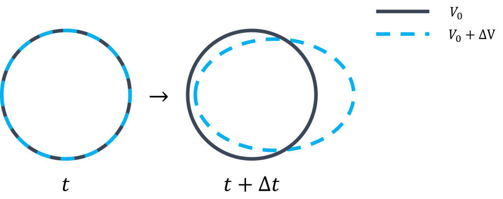
Consider the circle on the left, which is shown for some point in time at t. You could think that the circular boundary we see is the boundary of a collection of atoms. Let’s assume that we are now imparting a force on these atoms, and as a result, they start to move. Intuitively, we can say that these atoms will not move in a static fashion but rather. in a fluid sense, and thus, after some time t+\Delta t, the boundary of all the atoms has changed as seen on the right-hand side of the figure.

It is then also logical to conclude that if a collection of atoms is moving through space, its boundary is constantly changing. If we were to measure the area or volume of the boundary containing all of these atoms, it would be changing over time as well. Mathematically speaking, we can express that as V_0+\Delta V, where V_0 is the volume of the boundary at time t and \Delta V the differenfe in volume after we have advanced to t+\Delta t.

There are two types of flow properties

• Extensive flow properties: This property depends on the size of the system. The mass is an example. If you simulate a river or a system of rivers and lakes, you would expect the mass of water to be different in both cases
• Intensive flow properties: This property does not depend on the size of the system. The density is an example, and in the example above, we would expect the density of water to be the same for either type of simulation setup.

Let us now consider an extensive flow property (mass, volume, energy, etc.) and call it by the variable \Phi. In fluid mechanics, we like to talk about conserved flow quantities within a control volume, which essentially says that if we draw an arbitrarily small boundary around a portion of our system (a so-called control volume), we say that properties within this control volume can be regarded as constant. It is the mathematical equivalent of saying “we take an average”. This can be expressed in mathematical terms as:

\Phi = \int_V \phi \mathrm{d}V

This makes intuitive sense. Extensive properties depend on the system size, e.g. the mass of water contained within a volume of 1 m^3 will be different compared to that of the volume of 10 m^3 (assuming the density remains the same). Thus, the above equation simply states that when we increase or decrease the volume of the system through the integral \int_V\mathrm{d}V, then this change in volume is directly proportional to changes in \Phi.

There is a proportionality factor \phi, which depending on \Phi will take different forms. For example, if we consider \Phi to be mass, then \phi becomes the density of the fluid, which is commonly abbreviated as \rho. In an equation, this can be expressed as:

m = \int_V \rho\cdot \mathrm{d}V

This makes sense as a density multiplied by a volume provides a mass. This can also be easily seen by just looking at the units

\left[kg\right]=\left[\frac{kg}{\sout{m^3}}\right]\cdot\left[\sout{m^3}\right]

Here, we are assuming that \Phi is our mass in kilograms and \phi our density in kilograms per cubic meter. The reason we used \Phi and \phi above is to make it more generic. As it turns out, we can use this equation for many other flow properties, and this will help us construct our conservation laws of mass, momentum, and energy, which form the basis for the Navier-Stokes equations.

I mentioned conservation of momentum, so let’s take a look at that. In this case, we have \Phi=m\mathbf{u}, which represents the overall momentum (here, \mathbf{u} represents the velocity vector, and I use the convention here that a vector quantity is written with bold letters). We have already seen the link between mass and density, so we have \phi=\rho\mathbf{u}. In equation form, this results in:

m\mathbf{u}=\int_V \rho\mathbf{u}\cdot\mathrm{d}V

We can show, again, by just looking at units that this is correct

\left[kg\cdot\frac{m}{s}\right]=\left[\frac{kg}{\sout{m^3}}\cdot\frac{m}{s}\right]\cdot\left[\sout{m^3}\right]

We could have also taken the easy way by taking the equation we saw before for the mass conservation and multiplying that by the velocity vector \mathbf{u}. This would have resulted in the same equation.

So far, we have not done anything interesting, really. We essentially just stated mathematically that if we sum the density over a control volume, we get its mass, which we can intuitively verify. Then, we saw that we could multiply this equation by additional quantities to derive additional equations of interest. The equation that we looked at is static, but fluid dynamics (as the name suggests) is not static but rather a time-dependent problem. So we have to add the time derivative to either side to make this equation dynamic, and this results in:

\frac{\mathrm{d}\Phi(t)}{\mathrm{d}t}=\int_{V(t)}\frac{\mathrm{d}\phi}{\mathrm{d}t}\mathrm{d}V

This equation does provide us now with a time history, however, we have no idea (or means to measure) how the control volume is changing over time and thus we can’t solve the integral on the right-hand side, as the volume is now a function of time.

Whenever we are faced with a situation where we don’t know how a quantity is changing over time (or space), we can create a Taylor series for that quantity, which will give us an approximation to an unknown function. The idea is to replace the function we can’t solve analytically and approximate that with a function that looks fairly similar, at least within a small interval. We can then use this approximate function to determine properties such as derivatives, which will be similar to our original, unknown function.

In its most basic form, the Taylor series is written as

\phi(t+\Delta t) = \phi(t) + \frac{\mathrm{d} \phi}{\mathrm{d} t}\frac{\Delta t}{1!} + \frac{\mathrm{d}^2 \phi}{\mathrm{d} t^2}\frac{\Delta t}{2!} + \frac{\mathrm{d}^3 \phi}{\mathrm{d} t^3}\frac{\Delta t}{3!} + ... + \frac{\mathrm{d}^n \phi}{\mathrm{d} t^n}\frac{\Delta t}{n!}

Here, we are interested in a function \phi, for which we don’t know the exact functional relationship. We may know the function values at discrete points, e.g. at time t, but we may want to get a value for some point in time in the future at t+\Delta t. A classic example is where \phi is the temperature, and we know the temperature right now (i.e. we know \phi(t)), and we want to know what the temperature is tomorrow at t+\Delta t.

If we have no idea what the temperature is going to be tomorrow, but we know the measurement of today’s measurement, then the best guess we may have is that the temperature is going to be the same as today. It is not going to be 100% accurate, but we won’t be far off either. This is the first term in the Taylor series, i.e. if we want to get an approximation for \phi(t+\Delta t), then we may say that it is equal to \phi(t) (ignoring all other terms).

However, we may have yesterday’s temperature available as well, and we can see if the temperature is rising or falling. In other words, we know the slope of the temperature curve, which is nothing else than the derivative, which is the second term in the Taylor series. Combining this with the first term, we get

\phi(t+\Delta t) \approx \phi(t) + \frac{\mathrm{d} \phi}{\mathrm{d} t}\frac{\Delta t}{1!}

If we had even more information about past measurements, we could add more and more higher-order derivatives to get an ever increasing accuracy, as long as our \Delta t is small enough. Even if I had all the derivatives available, I probably still wouldn’t get an accurate prediction for the temperature if I tried to forecast it years in advance. But for a few days, we can get a good estimate.

Typically, we truncate the Taylor series after a few terms and express the terms we have dropped by the (and its highest exponent) by \mathcal{O}(\Delta x)^n, where n is the lowest-order term we are dropping. It is of no great importance to our understanding, but if you see this term, it just means we have dropped some additional terms. We have to, as the Taylor Series is an infinite series!

The following animation shows how the approximation of the exponential function f(x)=e^x improves as we add higher-order derivatives (the value of n corresponds to the derivatives in the Taylor series):

As we add more and more derivatives, the approximation becomes better and better. However, most of the time, our time step size \Delta t is rather small, so it is usually sufficient to consider only the first two terms (the constant and linear contribution). This can be expressed as:

\phi(t+\Delta t) = \phi(t) + \frac{\mathrm{d} \phi}{\mathrm{d} t}\frac{\Delta t}{1!} + \mathcal{O}(\Delta t)^2

We can rearrange this equation and write:

\frac{\phi(t+\Delta t) - \phi(t)}{\Delta t} =  \frac{\mathrm{d} \phi}{\mathrm{d} t} + \mathcal{O}(\Delta t)^2

Ignoring the higher order terms, we can further write the following approximation:

\frac{\mathrm{d} \phi}{\mathrm{d} t} \approx \frac{\phi(t+\Delta t) - \phi(t)}{\Delta t}

This approximation is valid for small \Delta t values. If we wanted to have an exact derivative, then we require that \Delta t\rightarrow 0, which we can express in the form of a limit, i.e. \lim\limits_{\Delta t\rightarrow 0}.

Returning now to our time-dependent formulation of \Phi, i.e.

\frac{\mathrm{d}\Phi(t)}{\mathrm{d}t}=\int_{V(t)}\frac{\mathrm{d}\phi}{\mathrm{d}t}\mathrm{d}V

We can see how we can split the right-hand side into two separate integrals. We simply replace the time derivative by its approximation and require the time-step to go towards zero. While the limit is inconsequential for our discussion, it is required from a mathematical consideration; otherwise, we will no longer be solving the same equation.

\frac{\mathrm{d}\Phi(t)}{\mathrm{d}t}=\lim\limits_{\Delta t\rightarrow 0}\left\{ \int_{V_0 + \Delta V} \frac{\phi(t + \Delta t)}{\Delta t}\mathrm{d}V - \int_{V_0} \frac{\phi(t)}{\Delta t}\mathrm{d}V \right\}

We can take the time step outside the brackets, which results in:

\frac{\mathrm{d}\Phi(t)}{\mathrm{d}t}=\lim\limits_{\Delta t\rightarrow 0}\frac{1}{\Delta t}\left\{ \int_{V_0 + \Delta V} \phi(t + \Delta t)\mathrm{d}V - \int_{V_0} \phi(t)\mathrm{d}V \right\}

Here, we have simply introduced the approximation of \mathrm{d} \phi /\mathrm{d} t and placed \Delta t outside the integration as it remains constant. Note that because the volume can change for some t + \Delta t, the integration is carried out over V_0 + \Delta V, while the integration at t can be taken over V_0.

We can expand the first of the two integrals and arrive at

\frac{\mathrm{d}\Phi(t)}{\mathrm{d}t}=\lim\limits_{\Delta t\rightarrow 0}\frac{1}{\Delta t}\left\{ \int_{V_0} \phi(t + \Delta t)\mathrm{d}V + \int_{\Delta V} \phi(t + \Delta t)\mathrm{d}V - \int_{V_0} \phi(t)\mathrm{d}V \right\}

This allows us to group together integrals of the same bounds (i.e. here \int_{V_0}). By doing so, we can write the above equation as

\frac{\mathrm{d}\Phi(t)}{\mathrm{d}t}=\lim\limits_{\Delta t\rightarrow 0}\frac{1}{\Delta t}\left\{ \int_{V_0} \left[ \phi(t + \Delta t) - \phi(t) \right] \mathrm{d}V + \int_{\Delta V} \phi(t + \Delta t)\mathrm{d}V \right\}

We want to obtain an expression for the left-hand side that we can readily solve, which is easier if we remove the limit from the right-hand side. So, let’s examine how we can achieve that. To get started, we expand the above equation and write the limit in front of each integral. This will allow us to evaluate each integral on its own. We have

\frac{\mathrm{d}\Phi(t)}{\mathrm{d}t}=\lim\limits_{\Delta t\rightarrow 0}\frac{1}{\Delta t}\int_{V_0} \left[ \phi(t + \Delta t) - \phi(t) \right] \mathrm{d}V + \lim\limits_{\Delta t\rightarrow 0}\frac{1}{\Delta t} \int_{\Delta V} \phi(t + \Delta t)\mathrm{d}V

Let us now look at the first integral. First, let’s reintroduce \Delta t back into the integral. Remember, a constant can be written before or after the integral. This results in:

\frac{\mathrm{d}\Phi(t)}{\mathrm{d}t}=\lim\limits_{\Delta t\rightarrow 0}\int_{V_0} \frac{\phi(t + \Delta t) - \phi(t)}{\Delta t} \mathrm{d}V + \lim\limits_{\Delta t\rightarrow 0}\frac{1}{\Delta t} \int_{\Delta V} \phi(t + \Delta t)\mathrm{d}V

A few equations ago, we have already established the following relationship through the Taylor series

\frac{\mathrm{d} \phi}{\mathrm{d} t} = \lim\limits_{\Delta t\rightarrow 0}\frac{\phi(t+\Delta t) - \phi(t)}{\Delta t}

Thus, we can simply rewrite the first integral as the time derivative, which will remove the limit from the integral. This is given as

\frac{\mathrm{d}\Phi(t)}{\mathrm{d}t}=\int_{V_0} \frac{\mathrm{d} \phi}{\mathrm{d} t} \mathrm{d}V + \lim\limits_{\Delta t\rightarrow 0}\frac{1}{\Delta t} \int_{\Delta V} \phi(t + \Delta t)\mathrm{d}V

Great, but what about the second integral? How do we integrate \phi(t + \Delta t)? Well, we don’t know the value of that function at some point in the future, so what do we do? Exactly, a Taylor series! Let’s expand the second integral then with a Taylor Series, this results in:

\frac{\mathrm{d}\Phi(t)}{\mathrm{d}t}=\int_{V_0} \frac{\mathrm{d} \phi}{\mathrm{d} t} \mathrm{d}V + \lim\limits_{\Delta t\rightarrow 0}\frac{1}{\Delta t} \int_{\Delta V}\left[ \phi(t) + \frac{\partial \phi}{\partial t}\frac{\Delta t}{1!} + \mathcal{O}(\Delta t)^2 \right]\mathrm{d}V

Remember, we still have the limit in front of the integral, and the limit requires \Delta t to go to zero. Hence, any term involving \Delta t has to go to zero (if you want to visualise, just set \Delta t=0 and then see which terms go to zero, you will see, it is the first derivative (and any higher-order derivative). What remains is the constant part of the Taylor series, which results in:

\frac{\mathrm{d}\Phi(t)}{\mathrm{d}t}=\int_{V_0}\frac{\mathrm{d} \phi}{\mathrm{d} t}\mathrm{d}V+\lim\limits_{\Delta t\rightarrow 0}\frac{1}{\Delta t}\int_{\Delta V} \phi(t)\mathrm{d}V

What just happened? Didn’t we say we can get rid of the limit? Well, not quite yet, we have to reformulate our equation a bit, otherwise if we let the time step to go to zero, the term 1/\Delta t would reach infinity, which makes the equation rather useless. So we need to reformulate this integral a bit.

The trick is to replace the volume integral with a surface integral, and in the process, we can let the limit go to zero for the time step without destroying our equation. To see how this can be done, let’s look at the volume first. It can be written as a product of an area and a length by which this area is extruded:

V=A\cdot L

A length L can be seen as a measure of a speed multiplied by time, and inserting this into our equation results in:

V=A\cdot\mathbf{u}\Delta t

We can make our volume and area infinitesimally small, which we can write as:

\mathrm{d}V=\mathrm{d}A\cdot\mathbf{u}\Delta t

This equation holds true regardless of the size of the element we are considering. We can now substitute our volume integral with a surface integral using the above expression, which results in:

\frac{\mathrm{d}\Phi(t)}{\mathrm{d}t}=\int_{V_0}\frac{\mathrm{d} \phi}{\mathrm{d} t}\mathrm{d}V+\lim\limits_{\Delta t\rightarrow 0}\frac{\Delta t}{\Delta t}\int_{A}\phi\mathbf{u}\mathrm{d}A

We can see that \Delta t / \Delta t is unity and thus will no longer influence the limit. We can drop the limit entirely from our equation to arrive at

\frac{\mathrm{d}\Phi(t)}{\mathrm{d}t}=\int_{V_0}\frac{\mathrm{d} \phi}{\mathrm{d} t}\mathrm{d}V+\int_{A}\phi\mathbf{u}\mathrm{d}A

The above equation is known as the Reynolds Transport Theorem and tells us how a quantity \Phi changes in space and time within a fluid. We can rewrite the Reynolds transport theorem for the second integral using Gauss’ (or divergence) theorem, which allows us to transform surface integrals back into a volume integral, which provides us with:

\frac{\mathrm{d}\Phi(t)}{\mathrm{d}t}=\int_{V_0}\frac{\mathrm{d} \phi}{\mathrm{d} t}\mathrm{d}V + \int_{V}\nabla\cdot\phi\mathbf{u}\mathrm{d}V

This form is particularly useful if we want to derive a differential form of the Reynolds transport theorem. This can be achieved by requiring that the control volumes we are looking at to become zero, i.e. V \rightarrow 0. In this case, we obtain

\frac{\mathrm{d}\Phi(t)}{\mathrm{d}t}=\frac{\mathrm{d} \phi}{\mathrm{d} t}+\nabla\cdot\phi\mathbf{u}

This is the final (differential) form of the Gauss (or divergence) theorem. Together with its integral form stated above, it is used in pretty much any equation we solve in CFD, from our conservation laws of mass, momentum, and energy to turbulence models, passive scalars, multiphase equations, and so on. Deriving any transport equation without the Reynolds transport theorem would be very difficult.

In the literature, you will find different names for \mathrm{d}\Phi(t)/\mathrm{d}t. It is either referred to as the total derivative, the substantial derivative or the material derivative. All of these denote the same thing, and when you read the literature, you may come across these different names.

Deriving the Navier-Stokes equations

Now that we have spent some time deriving the Reynolds Transport Theorem, we can put it to use to derive the governing equations of fluid dynamics, i.e. the Navier-Stokes equations. Strictly speaking, the Navier-Stokes equation is only concerned with the conservation of momentum. However, nowadays we use the term “the Navier-Stokes equations” to signal the conservation laws of mass (continuity), momentum, and energy.

In this section, we look at the conservation of mass and momentum, which are the fundamental building blocks for any CFD simulation. If we are interested in temperature effects, or we are using a compressible formulation in which the density may change, then we need the energy equation, but a bulk of the problems occurring in CFD can be solved with just the conservation of mass and momentum, and these are the equations we will have a look at in the next sections.

Conservation of Mass

We have already done all the heavy lifting and derived the Reynolds Transport theorem; deriving a conservation law for mass simply requires applying this theorem.

We also saw before that if we want \Phi to be the mass, then we need to set \phi=\rho. Thus, we write the Reynolds Transport Theorem as

\frac{\mathrm{d}m}{\mathrm{d}t}=\frac{\partial \rho}{\partial t}+\nabla\cdot\rho\mathbf{u}=0

We have made two changes here. The first change is the usage of a partial derivative \partial/\partial t instead of an ordinary derivative \mathrm{d}/\mathrm{d} t. We do that as \rho can not just change in time but also in space. Thus, we need to use the partial derivative whenever we have a derivative that depends on more than one variable.

Secondly, we set this equation to zero. This is because we want this to be a conservation law (the overall mass should not change), which means that the quantities on the left-hand side of the equations have to be conserved, and this is achieved by setting the right-hand side to zero. If the right-hand side was not equal to zero, the mass would either increase or decrease over time, violating the conservation of mass requirement. Thus, the conservation of mass, or continuity equation, can simply be written as

\frac{\partial \rho}{\partial t}+\nabla\cdot(\rho\mathbf{u})=0

This equation describes, in general, how mass is conserved. We will take special considerations into account at the end of this article to show how it may change for different flow regimes.

For an incompressible fluid, we say that the density is constant. If the density is constant, then there is no variation in time (by definition), so the time derivative becomes zero and can be neglected. We are then left with:

\nabla\cdot(\rho\mathbf{u})=0

Since \rho=const., we can also divide by it, which will further simplify our equation to

\nabla\cdot\mathbf{u}=0

This is the mass conservation law for an incompressible fluid and is only applicable to these types of flows. It is an important concept that will help us simplify other conservation laws encountered in incompressible flows.

Conservation of Momentum

The following section will deal with deriving the Navier-Stokes equation in full. We won’t make any assumptions and will dig deep into the literature, and I’ll show you the assumptions that Navier and Stokes made, which are typically not given in any derivation or textbooks. It’s a fascinating equation, and once you understand each step in the derivation, you will appreciate the complexity (but also its beauty) even more! Let’s dive in. It is going to be a fun exercise!

Starting with a molecular description

Before we jump into the conservation of momentum, let us take a step back and see the world through atoms. This is what Navier did to derive the momentum equation, and hey, if it is good enough for this french bloke, it’ll be good enough for us as well I suppose!

Picture a collection of particles floating in space without any forces acting on them apart from their electrostatic interactive forces. Such a collection of atoms will adhere to random fluctuations that, on average, cancel out so that there is no net movement when observing a large collection of atoms at the same time.

How could we force these atoms into motion? Well, we apply a force on each atom in a specific direction (this could be a magnetic force, for example). A heavier atom will have more inertia than a lighter atom, so the heavier atoms will take longer to accelerate than a lighter atom.

If this makes sense to you, then you are already at the same level as Navier and Stokes. From this observation, we can then start to look for an equation that describes the motion of each atom, and we quickly arrive at Newton’s second law, which is given as:

\mathbf{F}=m\mathbf{a}

Here, \mathbf{F} is the sum of the internal and external forces acting on the system and \mathbf{a} the acceleration. We could say that this equation describes any type of fluid, at least on a per-atom basis. It is, indeed, this equation that we solve in most particle-based approaches, such as molecular dynamics and the dissipative particle dynamics approach. However, we don’t want to describe the motion for each atom, but rather for a collective continuum of particles, and so we need to expand Newton’s second law.

What forces are acting on my system?

The first thing we have to look at is the force term. The question is, what type of forces are acting on our system? Typically, this is separated into two broad categories: internal and external forces, and this can be written as

\mathbf{F} = \mathbf{F}_{internal} + \mathbf{F}_{external}

External forces

Let’s look at the external forces first, then. The external forces describe anything that acts on our system, but our Navier-Stokes equations do not explicitly capture that. It acts on each fluid particle (or, if we run a CFD simulation, on each cell of our computational domain). Think of two immiscible fluids, where the heavy fluid is sitting on top of the light fluid, as shown in the video below

But think about where the “force” is coming from in order for the heavier fluid to penetrate into the lighter fluid. If we just solve the Navier-Stokes equations without any external forces, nothing would happen. But at this point, we can all agree that gravity is pulling the heavier fluid into the lighter fluid. Thus, gravity is one such external force that we can consider.

This also provides an additional point to consider; if we do not expect gravity to be important for us in our situation (i.e. simulation), then it is OK to neglect the external forces such as gravity. But when we derive the conservation of momentum, we want to keep all those terms and then drop them later if we think this is appropriate.

Similar to gravity, there are other forces acting on the fluid, which are typically termed body forces, i.e.

\mathbf{F}_{external} = \mathbf{F}_{gravity} + \mathbf{F}_{body}

Examples of body forces are magnetic fields, which influence the trajectory of magnetised fluid particles, and the Coriolis force, which imparts momentum in a specific direction to the fluid particles. Essentially, anything that would translate into additional momentum on fluid particles is lumped together into the body forces (and in some derivation, gravity is part of that body force term).

Internal forces

The internal forces are a bit more complicated and require some further considerations. Let’s think about a simplified system: we have two solid blocks, one sitting on top of the other. The block on top will assert a pressure force on the block below (similar to the heavier and lighter fluid situation above). The block below will assert the same pressure force back according to Newton’s third law (when two bodies interact with each other, they will apply an equal force to each other in the opposite direction). So, one such internal force is the pressure (force) itself.

Now, let’s imagine we were to push that block on top forward so that there would be friction between these two blocks. This friction force is due to the upper block shearing over the bottom block, and we feel that it is a resistance when pushing the upper block. This is referred to as the shear force or the shear stresses. The internal forces can thus be summarised as:

\mathbf{F}_{internal} = \mathbf{F}_{pressure} + \mathbf{F}_{shear stresses}

In summary, we have forces of all different forms and shapes. In the following derivation, we will carry over internal, gravity, and body forces for the remaining derivation. Let’s look at these terms in turn.

The internal force contains the pressure and shear stresses. From a dimensions-based analysis, we know that shear stresses are defined, according to Newton, as

\tau=\mu\frac{\partial\mathbf{u}}{\partial\mathbf{x}}\rightarrow\left[\frac{kg}{m\cdot s}\right]\cdot\left[\frac{m}{m\cdot s}\right]=\left[\frac{kg}{m\cdot s^2}\right]=\left[\frac{kg\cdot m}{m^2\cdot s^2}\right]=\left[\frac{N}{m^2}\right]

If we now were to take the derivative of \tau as in \nabla\cdot\tau, then we would obtain units of N/m^3. Integrating that over a volume would result in N, which is the correct unit for a force. Thus, we can write that

\mathbf{F}_{internal} = \int_{V}\nabla\cdot\sigma\mathrm{d}V

Here, we have chosen to represent all internal forces by \sigma, which includes not just the shear stresses but also the pressure forces. We will return to this point later. We do the volume integral here as the internal force is not a constant but may vary over our entire system’s volume. Integrating overall contributions will result in the overall internal force.

Gravity has units of m/s^2, and thus, we need to multiply it with some mass to get units of kg\cdot m/s^2=N. But since we are also going to integrate over the system’s volume (similar to the internal forces), we need to divide this force by units of m^3, which means we need to multiply our gravitational force by something of units kg/m^3, which is just the density \rho. Therefore, the gravitational force becomes

\mathbf{F}_{gravity} = \int_{V}\rho\mathbf{g}\mathrm{d}V

The body forces are provided as forces themselves and have units of N. Thus, we have to simply divide them by the system’s volume to account for the volume integral as in the cases before and arrive at

\mathbf{F}_{body} = \frac{1}{V}\int_{V}\mathbf{f}_{body}\mathrm{d}V

Thus, in summary, we can write the overall force as a superposition of the internal, gravitational, and body forces as

\mathbf{F} = \mathbf{F}_{internal} + \mathbf{F}_{gravity} + \mathbf{F}_{body} =
\int_{V}\nabla\cdot\sigma\mathrm{d}V + \int_{V}\rho\mathbf{g}\mathrm{d}V +
\frac{1}{V}\int_{V}\mathbf{f}_{body}\mathrm{d}V

This covers the left-hand side of Newton’s second law, i.e.

\mathbf{F} = \mathbf{F}_{internal} + \mathbf{F}_{external}=m\mathbf{a}

Deriving the general momentum equation

Now, we need to work on the right-hand side. As we saw previously, we want to integrate over the entire system’s volume to account for each change in mass and acceleration. After all, that is exactly what a conservation law is there for, i.e., to account for all contributions over a specific volume and track any changes. Since a volume integral will add units of m^3, we can divide the mass by a volume at this stage so that it will become a mass again after being multiplied by a volume. Dividing mass by a volume results in the density, thus:

\int_V\mathbf{F}\mathrm{d}V=\int_V\rho\mathbf{a}\mathrm{d}V

Taking a units-based approach again, we can see that the acceleration a has units of m/s^2, and we can replace this term with the time derivative of the velocity, which is easier for us to measure. This can then be written as

\int_V\mathbf{F}\mathrm{d}V=\int_{V}\frac{\mathrm{d} \rho\mathbf{u}}{\mathrm{d} t}\mathrm{d}V

At this stage, we simply insert the definitions for the forces we developed above and apply the Reynolds Transport Theorem derived previously to the right-hand side, where we use \Phi=\rho\mathbf{u}. We do that because we are interested in how \rho\mathbf{u} changes over time, which is what the Reynolds transport theorem tells us. We also switch the equation around so that the time derivative is on the left-hand side while all force terms are collected on the right-hand side. This results in

\int_{V}\frac{\partial \rho\mathbf{u}}{\partial t}\mathrm{d}V + \int_{V}\nabla\cdot (\rho\mathbf{u}\otimes\mathbf{u})\mathrm{d}V = 
\int_{V}\nabla\cdot\sigma\mathrm{d}V + \int_{V}\rho\mathbf{g}\mathrm{d}V + \frac{1}{V}\int_{V}\mathbf{f}_{body}\mathrm{d}V

You’ll have noticed that we now have this \nabla\cdot (\rho\mathbf{u}\otimes\mathbf{u}) term, where did this new special character \otimes come from? This is known as the dyad product, and we have to use it as we are now multiplying two vectors. To see why we need this dyad (or tensor) product, let’s look at the Reynolds transport theorem again:

\frac{\mathrm{d}\Phi(t)}{\mathrm{d}t}=\frac{\mathrm{d} \phi}{\mathrm{d} t}+\nabla\cdot\phi\mathbf{u}

In our case, we set \phi=\mathbf{u}, so the time derivative will now be a vector itself (containing the time derivatives of the velocity vector in the x, y, and z velocity components, if we use a Cartesian coordinate system). If we simply inserted \phi=\rho\mathbf{u} for the second term, we would get \nabla\cdot\rho\mathbf{u}\mathbf{u}. Multiplying two vectors together results in a scalar using the dot or scalar product.

If we were to do that, we would have a vector quantity for the time derivative and a scalar quantity for the second term. From basic vector calculus, we know that we can’t add a vector and a scalar (we can only multiply them), so the second term has to retain a vector-like shape. We achieve that with the dyad product, which will result in a second-rank tensor (which is dirty math talk for “it’s a matrix”, and my sloppy use of language here will, I am sure, upset some mathematicians. I know there is a difference between the two, but it is beside the point here).

Let’s look at this dyad product in more detail. We can formally introduce it as

a\otimes b=\begin{bmatrix}a_1b_1 & a_1b_2 & a_1b_3 \\a_2b_1 & a_2b_2 & a_2b_3 \\a_3b_1 & a_3b_2 & a_3b_3 \\\end{bmatrix}

Since both the time derivative and now the convective term (i.e. the second term in the Reynolds transport theorem) now have three components in the x, y, and z direction, we can add them together again. So, if we want to insert vector quantities into our Reynolds transport theorem, we need to remember to carry out a tensor (dyad) product so we end up with the correct equation structure (tensor instead of a scalar).

Returning to our intermediate momentum equation above, we can carry out the integration over the volume and realise that the volume appears in each term. Thus, we divide by the volume to arrive at the following general momentum conservation equation (which is also known as the Cauchy momentum equation)

\frac{\partial \rho\mathbf{u}}{\partial t} + \nabla\cdot (\rho\mathbf{u}\otimes\mathbf{u}) = \nabla\cdot\sigma+\rho\mathbf{g}+\frac{1}{V}\mathbf{f}_{body}

The above equation is written in conservative form; that is, all quantities are contained within the derivatives. However, the Navier-Stokes equation is commonly written in the so-called convective form, so let’s see how we can arrive at this form instead. To do that, we need one general rule of differential calculus and one vector identity, which are given below:

(ab)'=ab'+a'b\\\nabla\cdot(\mathbf{a}\otimes\mathbf{b})=(\nabla\cdot\mathbf{a})\mathbf{b}+\mathbf{a}\cdot\nabla\mathbf{b}

Here, ()' indicates that we want a time derivative of a quantity provided within the parenthesis. To make things simple, let’s set the entire right-hand side to S=\nabla\cdot\sigma+\rho\mathbf{g}+\mathbf{f}_{body}/V, so we can concentrate on the left-hand side only. The first vector identity applies to the time-derivative, and so we can write:

\rho\frac{\partial \mathbf{u}}{\partial t} + \mathbf{u}\frac{\partial \rho}{\partial t} + \nabla\cdot (\rho\mathbf{u}\otimes\mathbf{u}) = S

Inserting the dyad vector identity, we can rewrite the second term as:

\rho\frac{\partial \mathbf{u}}{\partial t} + \mathbf{u}\frac{\partial \rho}{\partial t} + (\nabla\cdot\rho\mathbf{u})\mathbf{u}+\rho\mathbf{u}\cdot\nabla\mathbf{u} = S

Now, we can factorise the equation to arrive at the following form:

\mathbf{u}\left(\frac{\partial \rho}{\partial t}+\nabla\cdot\rho\mathbf{u}\right) + \rho\left(\frac{\partial \mathbf{u}}{\partial t} +\mathbf{u}\cdot\nabla\mathbf{u}\right) = S

The first parenthesis must be equal to zero, as this is just our continuity (mass conservation) equation we derived above, and we saw that it was set to zero, so we can neglect this term. Thus, we can write the momentum equation that we have derived thus far in the following convective form, which is, as stated above, the common way to write the Navier-Stokes equations:

\rho\frac{\partial \mathbf{u}}{\partial t} + \rho(\mathbf{u}\cdot\nabla)\mathbf{u} = \nabla\cdot\sigma+\rho\mathbf{g}+\frac{1}{V}\mathbf{f}_{body}

A simplistic approach: the Euler momentum equation

The crucial aspect in deriving the momentum conservation laws for fluids is how we treat the internal forces, i.e. how we define \sigma. We said that \sigma contains all pressure and internal shear forces, which we can express as

\sigma = -p\mathbf{I} + \tau

Here, the pressure p is a scalar value. Since the pressure forces can only act normal to surfaces (not tangential to them), we multiply it by the identity matrix \mathbf{I} to ensure it is only acting normal to the x, y, and z direction. The pressure is also a scalar value, meaning that its value is the same in the x, y, and z direction.

The shear stresses \tau, on the other hand, form a tensor (again, essentially a matrix, but let’s not wind up those mathematicians more than we have to), so we can see the necessity to provide the pressure in a matrix form as well so that we can add both terms together.

We could make life simple for us and say that the shear stresses are zero, i.e. \tau=0, which would result in \sigma = -p\mathbf{I}. In this case (omitting also any external forces), we can write our momentum equation as:

\rho\frac{\partial \mathbf{u}}{\partial t} + \rho(\mathbf{u}\cdot\nabla)\mathbf{u} = -p\mathbf{I}

This is known as the Euler equation, i.e. this equation is valid for inviscid flows only, which is a crude but reasonable approximation for high-speed flows. If you want to write a compressible flow solver, starting with the Euler equations is usually not a bad idea as it will convey the basic characteristics of the flow you are solving. For more general situations, though (especially if we are interested in turbulence), it can’t capture what we are interested in!

So, thank you, Euler, but we have to leave you behind now and look at what Navier and Stokes did. They both arrived at the same equation, using slightly different reasons and being unaware of the work of the other (if only the internet existed in 1820-1850, seriously, what did people do back then without 5G?). Navier came up with the solution some 20 years before Stokes, but their work combined provided us with a useful equation that has proven to be a rather useful equation in determining the flow of a fluid.

Lucky bastard: Why history remembers the work of Navier but it shouldn’t!

The history of the development of Navier and Stokes is fascinating, well, at least to me, but I guess you would expect that of someone teaching the Navier-Stokes equation on a daily basis to students. But bear with me, there will be some new information for you I am sure even if you are already well familiar with the equation itself.

The Euler equation was long accepted in the 19th century, but the role of friction was not properly understood. Louis Marie Henri Navier, Jean Claude Barre de Saint-Venant, and George Gabriel Stokes all presented different approaches to extend the Euler equation to incorporate friction between fluid layers.

In his 1822 paper titled “Memoire sur les lois du mouvement des fluides”, Navier presented his hypothesis about diffusion to the Academie des Sciences in Paris, which was published five years later. His work was based on molecular considerations as mentioned above, and interestingly, Anderson (J. D. Anderson, “Brief History of the Early Development of Theoretical and Experimental Fluid Dynamics,” 2010., p.12) highlights that:

“Navier’s equations were of the correct form, [however, ] his theoretical reasoning was greatly flawed, and it is almost a fluke that he obtained the correct terms“.

Yes, indeed, Navier took a lucky shot at the problem, and surprisingly, there was some truth to his statements. It was not until 1843, seven years after Navier’s death, that Saint-Venant entered the picture and re-derived Navier’s hypothesis from a macroscopic point of view, completely ignoring the molecular considerations given by Navier. His derivations were sound and arrived at the correct form.

Around the same time, in 1845, Stokes published his hypothesis on diffusion in his paper titled “On the Theories of the Internal Friction of Fluids in Motion, and of the Equilibrium and Motion of Elastic Solids”. Stokes was unaware of the work of Navier or Saint-Venant, as alluded to above. Despite the more rigorous derivation given by Saint-Venant, the equations became known as the Navier-Stokes equations. Navier got lucky, and I suppose we could call Saint-Venant the Buzz Aldrin of fluid mechanics!

(Though Saint-Venant came before Buzz Aldrin, should we be calling Buzz Aldrin the Saint-Venant of space exploration?)

Almost there, but we need to talk about constitutive equations first

We have almost all the pieces of the puzzles lined up. We just need one final ingredient to be able to derive the Saint-Venant-Stokes, I mean, the Navier-Stokes equations (a little Freudian slip on my behalf, apologies).

A constitutive equation relates two or more physical quantities with each other. Fluid mechanics is full of them, we have, for example, the equation of state p=\rho R T, where the pressure can be expressed in terms of the density, the gas constant, and the temperature, or the drag force D=0.5 c_d \rho u_\infty^2 A, which is expressed in terms of a drag coefficient and reference area, as well as the density and freestream velocity.

Constitutive equations allow us to express one quantity we don’t know through other quantities we either know or can measure. These constitutive equations can be either derived from first principles (where we start with some fundamental physical law) or through empirical correlations.

An example where we derive the constitutive equation from first principle is the velocity profile in a 2D, laminar flow through a pipe. We start with the Navier-Stokes equation itself and then cancel out terms that are not relevant. The terms that remain in the Navier-Stokes equation can then be integrated and provide us with the famous laminar, quadratic velocity profile of the form:

u(r)=U_0\left(1-\frac{r^2}{R^2}\right)

where U_0 is the center line (max) velocity within the pipe, r is a coordinate along the radius of the pipe, and R is the radius of the pipe itself.

An example of an empirical constitutive equation is Poiseuille’s law, who stated that for the same pipe flows, we can determine the pressure drop within a pipe using the following formula:

\Delta p=128\frac{\mu L Q}{\pi d^4}

Here, we have \Delta p being the pressure drop, \mu the dynamic viscosity, L the length of the pipe over which we want to measure the pressure drop, Q the flow rate, and d being the diameter of the pipe. Where did the value of 128 come from? Well, measurements and the subsequent curve fittings.

Poiseuille postulated that all of these quantities play a role in the pressure drop, and the equation above approximates the pressure drop, but no fundament physical law was used to derive this equation.

So, now that we understand what a constitutive law is, we can move on and look at the momentum equation again.

Finding a constitutive equation for the shear stresses

Let’s start by inserting our definition of \sigma = -p\mathbf{I} + \tau into the Cauchy momentum equation. We obtain the following equation, which is exact (no approximation is done):

\frac{\partial \rho\mathbf{u}}{\partial t} + \rho(\mathbf{u}\cdot\nabla)\mathbf{u} = \nabla\cdot(-p\mathbf{I} + \tau)+\rho\mathbf{g}+\frac{1}{V}\mathbf{f}_{body}

We can then also separate the pressure and shear stress contribution to write the equation as:

\frac{\partial \rho\mathbf{u}}{\partial t} + \rho(\mathbf{u}\cdot\nabla)\mathbf{u} = -\nabla p + \nabla\cdot\tau + \rho\mathbf{g}+\frac{1}{V}\mathbf{f}_{body}

Here, we made use of the fact that taking the gradient of a scalar quantity is equivalent to multiplying that scalar with the identity matrix and then taking the divergence of that quantity, i.e. we used the following identity: \nabla\cdot (p\mathbf{I}) = \nabla p.

The work of Navier, Saint-Venant, and Stokes boils down to finding a suitable constitutive equation for the shear stresses \tau (and, if after reading the rest of this section and you feel inspired to come up with your very own constitutive equation, you can create your own momentum equation and call it whatever you want).

In 1686, Newton had an idea of how shear stresses ought to behave and put it in words, but it was not until 1845 that Stokes translated these words into a three-dimensional equation. Poiseuille also proved in 1856 through experiments that Newton’s hypothesis was true. Nowadays, we know this constitutive relation as Newton’s law of viscosity, but really, it was the work of Stokes, Saint-Venant (heck, even that chap called Navier), Poiseuille, Hagen, and Bingham, who should be remembered just as much for their contributions!

Newton’s law of viscosity can be stated (in 1D) as:

\tau=\mu\frac{\mathrm{d}u}{\mathrm{d}y}

That is to say, we can now approximate the shear stress through the dynamic viscosity (which we can measure), as well as the velocity profile (which we can also measure). Here, we assume that there is only one velocity gradient, but if we want to generalise this to 3D (which is effectively what Stokes did), then we could write this as a tensor instead:

\tau_{xy}=\mu\begin{bmatrix}\frac{\partial u}{\partial x} & \frac{\partial u}{\partial y} & \frac{\partial u}{\partial z} \\ \frac{\mathrm{d}v}{\partial x} & \frac{\partial v}{\partial y} & \frac{\partial v}{\partial z} \\ \frac{\partial w}{\partial x} & \frac{\partial w}{\partial y} & \frac{\partial w}{\partial z}\end{bmatrix}

Notice that our ordinary differential operator has now become a partial differential operator as the velocity components now depend on more than one variable (i.e. the x, y, and z direction, to be precise). We could also write this with our nabla notation as:

\tau_{xy}=\mu\cdot\nabla \mathbf{u}

Closely related to Newton’s law of viscosity is the strain rate. The strain rate is defined as \dot{\gamma}=u/h, where u is the relative velocity between two fluid layers in motion (typically taken between two solid plates in relative motion, i.e. the Couette flow) and h the distance between these two plates. Now, if we let the distance between these two plates go to zero, noting that the relative velocity can be expressed as the difference between the fluid velocity at the upper and lower layer, then we can write

\dot{\gamma}=\frac{u}{h}=\lim_{h\rightarrow 0}\frac{u_{upper}-u_{lower}}{h}=\frac{\mathrm{d}u}{\mathrm{d}h}

If we replace the height h with the more general variable x, then we can see that the strain rate is nothing else than the velocity gradient in disguise (in 1D), and the velocity gradient tensor in the more general 3D form. Thus, if we are able to measure the strain rate \dot{\gamma} and the shear stresses \tau, then we can plot their relationship and determine a mathematical model from that.

The following figure is taken from a study by B. C. Sahoo et al. 2009, where these two properties were measured in a lab for nanofluidic applications.

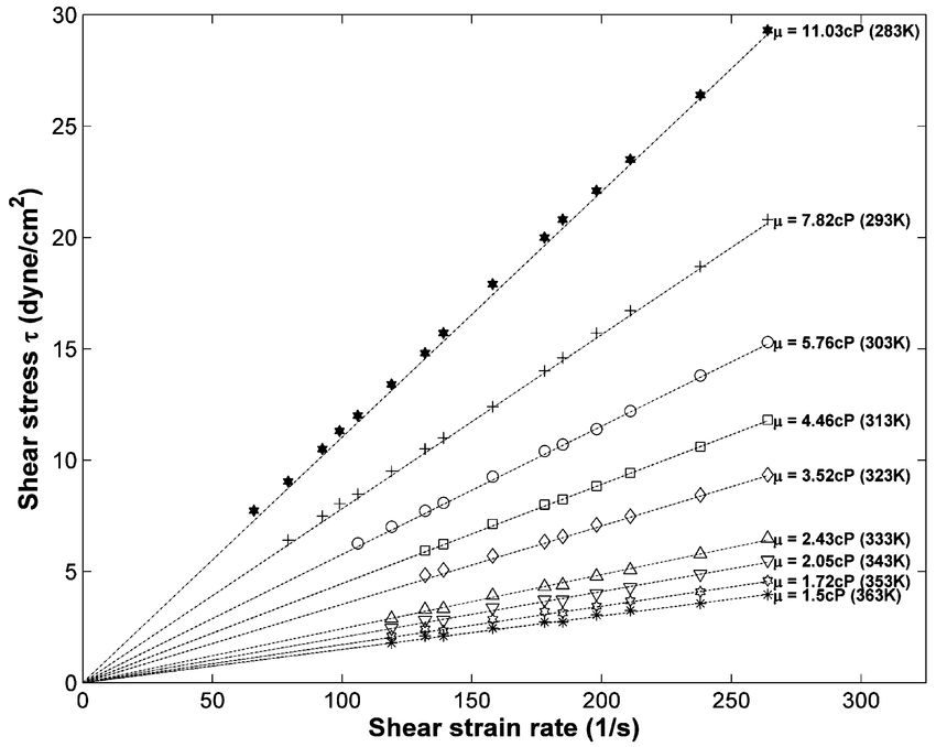
We can see that there are linear relationships for all of the measured lines, and we can also see that the steepness of these lines is determined by the dynamic viscosity \mu. This makes sense, as we have already seen from Newton’s law of viscosity that we expect a linear relationship between the shear stress and strain rate and that the dynamic viscosity is just a scaling factor.

And we could even do some linear curve fitting using the general equation for a linear line of

y=mx+b

In this case, we set b=0, as all curves pass through the origin, y=\tau, m=\mu, and x=\dot{\gamma}=\nabla\mathbf{u}. Inserting these quantities, we arrive again at Newton’s law of viscosity.

Stokes’ and Saint-Venant’ brilliance: How to treat internal forces

Ok, so we have a constitutive equation for the shear stresses, so we can just plug that into the momentum equation and then be done with it, right? Not quite, and if it was that simple, we’d probably call the Navier-Stokes equations the Newton equations of fluid dynamics instead! The crux is in the definition of the velocity gradient tensor \nabla\mathbf{u}, which we saw in Newton’s law of viscosity, which we need to decompose into a symmetric and an anti-symmetric part as

\nabla \mathbf{u}=\underbrace{\frac{1}{2}\left[\nabla \mathbf{u}+(\nabla \mathbf{u})^T\right]}_{symmetric}+\underbrace{\frac{1}{2}\left[\nabla \mathbf{u}-(\nabla \mathbf{u})^T\right]}_{anti-symmetric}

The above decomposition can be done for any matrix or second-order tensor, as shown by the mathematician Toeplitz. We can simply write out the tensors to verify that this can indeed be done. Introducing the shorthand notation \frac{\partial u}{\partial x}=u_x, we have

\nabla \mathbf{u}=\frac{1}{2}\begin{bmatrix}u_x & u_y & u_z \\ v_x & v_y & v_z \\ w_x & w_y & w_z\end{bmatrix}+\frac{1}{2}\begin{bmatrix}u_x & u_y & u_z \\ v_x & v_y & v_z \\ w_x & w_y & w_z\end{bmatrix}^T+\frac{1}{2}\begin{bmatrix}u_x & u_y & u_z \\ v_x & v_y & v_z \\ w_x & w_y & w_z\end{bmatrix}-\frac{1}{2}\begin{bmatrix}u_x & u_y & u_z \\ v_x & v_y & v_z \\ w_x & w_y & w_z\end{bmatrix}^T

We can see that the second and fourth tensors cancel out, and we are left with

\nabla \mathbf{u}=\frac{1}{2}\begin{bmatrix}u_x & u_y & u_z \\ v_x & v_y & v_z \\ w_x & w_y & w_z\end{bmatrix}+\frac{1}{2}\begin{bmatrix}u_x & u_y & u_z \\ v_x & v_y & v_z \\ w_x & w_y & w_z\end{bmatrix}=\begin{bmatrix}u_x & u_y & u_z \\ v_x & v_y & v_z \\ w_x & w_y & w_z\end{bmatrix}

This is the original velocity gradient tensor that we started with, confirming that Toeplitz’s decomposition does not change the original tensor. Let’s investigate the anti-symmetric part (which is the third and fourth tensor above). This can be written as

\frac{1}{2}\left[\nabla \mathbf{u}-(\nabla \mathbf{u})^T\right]=\frac{1}{2}\begin{bmatrix}u_x & u_y & u_z \\ v_x & v_y & v_z \\ w_x & w_y & w_z\end{bmatrix}-\frac{1}{2}\begin{bmatrix}u_x & u_y & u_z \\ v_x & v_y & v_z \\ w_x & w_y & w_z\end{bmatrix}^T = \frac{1}{2}\begin{bmatrix}u_x & u_y & u_z \\ v_x & v_y & v_z \\ w_x & w_y & w_z\end{bmatrix} - \frac{1}{2}\begin{bmatrix}u_x & v_x & w_x \\ u_y & v_y & w_y \\ u_z & v_z & w_z\end{bmatrix} =\\
\frac{1}{2}\begin{bmatrix}0 & u_y - v_x & u_z - w_x \\ v_x - u_y & 0 & v_z - w_y \\ w_x - u_z & w_y - v_z & 0\end{bmatrix}

Compare that to the definition of vorticity, which is related to the rotation of a fluid:

v=\nabla\times\mathbf{u}=\begin{bmatrix} w_y-v_z \\ u_z-w_x \\ v_x-u_y \end{bmatrix}

We can see that the anti-symmetric part of the velocity gradient tensor decomposition contains the same quantities, albeit some having the opposite sign. Stokes then assumed that, due to the rotational nature, the ani-symmetric part should be dropped in the definition of the shear stresses. Why? Well, let’s do a simple experiment to see why.

Suppose we have two vectors, which are a=[1, 0, 0] and b=[0, 1, 0]. If we now take the cross product of these two vectors, we have

\begin{bmatrix}1 \\ 0 \\ 0\end{bmatrix}\times\begin{bmatrix}0 \\ 1 \\ 0\end{bmatrix} = \begin{bmatrix}0\cdot 0-0\cdot 1 \\ 0 \cdot 0 - 1 \cdot 0 \\ 1 \cdot 1 - 0\cdot 0 \end{bmatrix} = \begin{bmatrix}0 \\ 0 \\ 1\end{bmatrix}

Let say that both of these vectors a and b form a plane, in this case, a plane that is aligned with the x and y coordinate direction, then, taking the cross product of these two vectors results in a vector that is normal to this plane (and aligned with the z direction). Thus, taking the cross product will always create a vector quantity that is normal to the plane that its underlying vectors span.

If we relate that to a fluid particle, a force that is normal to the fluid particle’s surface is a pressure force, but a force that is applied tangentially along the surfaces is a shear force. Normal forces like the pressure do not contribute to shearing forces.

Thus, the vorticity is acting normal to the plane its two vector component span, and thus, vorticity does not contribute to shear stresses. Therefore, we can drop the anti-symmetric part, as it simply contains the same velocity quantities as the vorticity vector.

For completeness, the velocity gradient tensor decomposition is sometimes also written as

\nabla \mathbf{u}=\underbrace{\frac{1}{2}\left[\nabla \mathbf{u}+(\nabla \mathbf{u})^T\right]}_{symmetric}+\underbrace{\frac{1}{2}\left[\nabla \mathbf{u}-(\nabla \mathbf{u})^T\right]}_{anti-symmetric} = \mathbf{S}+\mathbf{\Omega}

Here, \mathbf{S} represents the symmetric (strain) part, and \mathbf{\Omega} the anti-symemtric (rotational) part. After we have dropped \mathbf{\Omega}, we can write our constitutive equation for the shear stresses of a fluid in the following form:

\tau=2\mu \mathbf{S}=\mu[\nabla\mathbf{u}+(\nabla\mathbf{u})^T]

We have to multiply by a factor of two as both \mathbf{S} and \mathbf{\Omega} contribute an equal half to the tensor decomposition. Multiplying by two accounts for the fact that we have dropped \mathbf{\Omega}. Anyways, that is what Stokes assumed. If you want to challenge him on that, feel free to create your own constitutive equation.

In principle, we are done. The above equation works, but just not for all types of flows (most notably, compressible flows). In order to also treat those flows (and have a generalised form of the Navier-Stokes equation), we need to look at one last concept.

Stokes velocity due to dilatation

In his 1845 paper On the theories of the internal friction of fluids in motion, George Gabriel Stokes derived his hypothesis of how friction in a fluid comes about and used molecular considerations to arrive at his final equations. He assumed that the velocity can be decomposed as

Total Velocity = Velocity due to Translation + Velocity due to Rotation + Velocity due to Dilatation

The first two terms are the ones we have seen above, which were due to Toeplitz’s matrix decomposition into a symmetric and anti-symmetric part (note that the above is for the overall velocity, not shear stresses; hence, we do account for the rotation here again). The third term, velocity due to dilatation, requires a bit further explanation.

Stokes used a control volume approach, where the control volume itself is moving with the flow, specifically, with the mean velocity. If we make the control volume so small that we resolve individual atoms, then we would observe that these atoms do not have a preferred direction of movement since the control volume itself is moving with the mean flow. In other words, the atoms follow Brownian motion.

If we now consider these atoms to hit the walls of the control volume, they would cause the volume to expand, which is what dilatation is. This idea is shown schematically below:

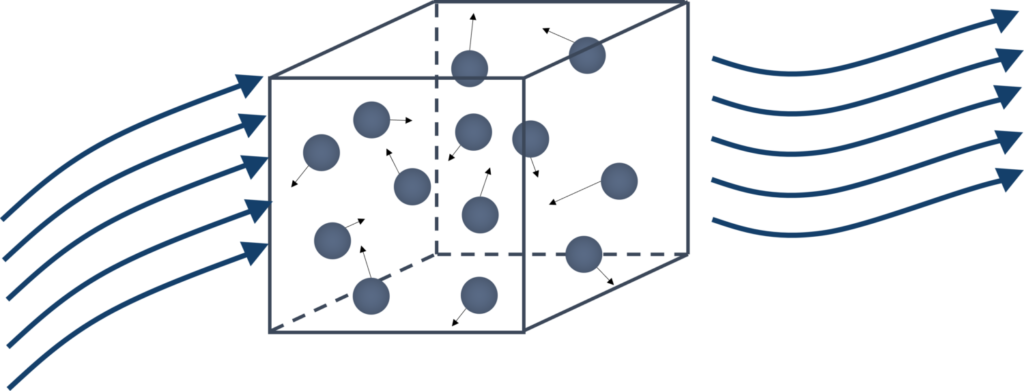
He then postulated that this dilatation term should be written as

\delta=\nabla\cdot\mathbf{u}=\frac{\partial u}{\partial x}+\frac{\partial v}{\partial y}+\frac{\partial w}{\partial z}

To understand how this equation comes about, we need first to understand how density works at a molecular level. When we deal with atoms, it makes more sense to talk about the number density, i.e. how many particles are within a given volume. In the figure above, we have 13 atoms drawn, so its number density would be 13 (for that control volume).

Let’s look at Stokes’ dilatation term above; it is the continuity equation! For an incompressible flow, we know that we have \nabla\cdot\mathbf{u}=0. Let’s say the u velocity component changes in the x direction so that \partial u/\partial x increases. This means that either \partial v/\partial y or \partial w/\partial z, or both, need to get smaller, so that we still have \nabla\cdot\mathbf{u}=0.

When \partial u/\partial x increases, that means that our control volume has to stretch in the x direction, and likewise, the control volume would shrink in the y and/or z directions. The number of particles would not change; they would still be in the control volume (by definition), so the number density (and, by extension, the macroscopic density) would remain constant. This is what we know to be true for an incompressible flow.

However, for a compressible flow, the density does not have to be constant, and this can also be related to the schematic above. If all three velocity gradients increase, i.e. \partial u/\partial x, \partial v/\partial y and \partial w/\partial z, then we would expect the control volume to increase. However, it will still contain the same number of atoms. The number density will reduce as the control volume increases, and so, by extension, the macroscopic density will decrease.

Therefore, if we expect a change in density, Stokes was saying that this will result in dilatation, and its effect contributes to the shear stresses. Since he decomposed the velocity into its translational, rotational, and dilatational part, its makes sense then (from a mathematical perspective), to include this additional term in our shear stress definition. This is done in the following:

\tau = \mu[\nabla\mathbf{u}+(\nabla\mathbf{u})^T]+\lambda(\nabla\cdot\mathbf{u})

In order to understand the additional new variable \lambda, which is referred to as the bulk viscosity, Stokes needed to make some further assumptions. He assumed that the dilatation is uniform, i.e. the control volume is expanding or contracting in each direction uniformly.

In our discussion above, we looked at individual components of the velocity gradient. We said they could change independently of each other, but that was purely done to get an insight into how the equation works. When we get to a molecular level, though, we discussed that particles are moving with no preferred direction of motion (once the mean flow is removed), which we introduced as Brownian motion.

Since there is no preferred direction of movement, we could also just look at one direction and then say that it is the same in the other directions, i.e. if we knew the velocity gradient component in the x direction, we could say it is the same in the other two directions. This is, anyway, what Stokes assumed to quantify the dilatation. Since each direction has the same strength and magnitude, we would need to multiply \nabla\cdot\mathbf{u} by a third to get just one direction, and this is what Stokes assumed as:

\delta = \frac{1}{3}\nabla\cdot\mathbf{u}

Next, Stokes also assumed that we can further write Newton’s shear stress equation as

\tau=2\mu[S-\delta]

A positive dilatation causes the control volume to increase. So, let’s think about what that would mean for the shear stresses. If the control volume increases, we are expanding its surface area on each side. The shear stresses have units of N/m^2, so if the surface area increases but everything else stays constant, then our shear stresses would have to decrease (purely from a dimensional consideration).

Thus, Stokes said that this decrease in shear stress will be achieved by subtracting the dilatation term rather than by adding it (which would result in larger shear stresses).

If we now insert Stokes’ hypothesis into our stress tensor, then we arrive at the final form of

\tau = \mu[\nabla\mathbf{u}+(\nabla\mathbf{u})^T]-\frac{2}{3}\mu(\nabla\cdot\mathbf{u})

At this point, I should stress again that this is a constitutive equation, i.e. something that Stokes, Saint-Venant, and Navier have come up with and we have found to work well for a range of applications, but that does not mean that they have provided us with a closure for the exact Cauchy momentum equation. Just because their mathematics looks elegant and we have found these equations to work well for a wide range of applications, we still don’t know if the above constitutive equation is indeed correct in a physical sense.

In fact, there is still a lively debate as to whether the -\frac{2}{3}\mu term is correct or not. The uniqueness and existence of the Navier-Stokes equations remains an open problem and is one of the seven unsolved problems listed by the Clay Institute, for which there is a 1 000 000 $ award to be claimed by someone able to provide proof of these equations. You can read about this on the Clay Institute website (and share your solution with me; sharing is caring, right? …).

Putting it all together: the final Navier-Stokes momentum equation

Taking the derivative of the above equation, the following result is obtained

\nabla\cdot\tau = \mu[\nabla\cdot\nabla\mathbf{u} + \nabla(\nabla\cdot\mathbf{u})] - \frac{2}{3}\mu\nabla(\nabla\cdot\mathbf{u})

Inserting this definition of the viscous stress tensor into \sigma = -p\mathbf{I} + \tau and then into the Cauchy momentum equation, and dividing all terms by the density, the following equation is obtained

\frac{\partial \mathbf{u}}{\partial t} + (\mathbf{u}\cdot\nabla)\mathbf{u} = -\frac{1}{\rho}\nabla p + \nu\nabla^2\mathbf{u} + \nu\nabla(\nabla\cdot\mathbf{u}) - \frac{2}{3}\nu\nabla(\nabla\cdot\mathbf{u}) + \mathbf{g} +\frac{1}{\rho V}\mathbf{f}_{body}

Here, \nu=\mu/\rho is the kinematic viscosity. Defining Q=\nu\nabla(\nabla\cdot\mathbf{u}) - \frac{2}{3}\nu\nabla(\nabla\cdot\mathbf{u}) + \mathbf{g} +\frac{1}{\rho V}\mathbf{f}_{body} as a source term, we can write the above equation as

\frac{\partial \mathbf{u}}{\partial t} + (\mathbf{u}\cdot\nabla)\mathbf{u} = -\frac{1}{\rho}\nabla p + \nu\nabla^2\mathbf{u} + Q

This is the conservation of momentum equation according to Navier, Saint-Venant, and Stokes, or, as we call it, the Navier-Stokes equation. Originally, the Navier-Stokes equation was simply that, i.e. the conservation of momentum, but these days, we also consider the conservation of mass and energy to be part of the set of Navier-Stokes equations, although Navier and Stokes had nothing to do with these conservation laws.

At this point, it is worthwhile to point out that the incompressible Navier-Stokes equations are obtained by realising that we got \nabla\cdot\mathbf{u}=0 from the continuity equation, and so if we insert that into our generalised Navier-Stokes momentum equation, i.e.:

\frac{\partial \mathbf{u}}{\partial t} + (\mathbf{u}\cdot\nabla)\mathbf{u} = -\frac{1}{\rho}\nabla p + \nu\nabla^2\mathbf{u} + \nu\nabla(\underbrace{\nabla\cdot\mathbf{u}}_{=0}) - \frac{2}{3}\nu\nabla(\underbrace{\nabla\cdot\mathbf{u}}_{=0}) + \mathbf{g} +\frac{1}{\rho V}\mathbf{f}_{body}

Removing the zero contributions from our equations results in the final form:

\frac{\partial \mathbf{u}}{\partial t} + (\mathbf{u}\cdot\nabla)\mathbf{u} = -\frac{1}{\rho}\nabla p + \nu\nabla^2\mathbf{u} +  \mathbf{g} +\frac{1}{\rho V}\mathbf{f}_{body}

Most of the time, this equation is simplified further by dropping body force terms and the influence of gravity (what we introduced as external forces), and we obtain the following simplified equation, which now only includes the internal forces:

\frac{\partial \mathbf{u}}{\partial t} + (\mathbf{u}\cdot\nabla)\mathbf{u} = -\frac{1}{\rho}\nabla p + \nu\nabla^2\mathbf{u}

Summary

So there you have it: the derivation of the Navier-Stokes equations in just under an hour. That’s not too bad! The key take-away messages are as follows:

• If we want to derive any transport equation, we need to consider the Reynolds transport theorem, which tells us how a quantity changes in time and space.
• Using the Reynolds transport theorem and applying it for the density, momentum, and energy, provides us with the set of equations that govern fluid dynamics, which we also know as the Navier-Stokes equations these days.
• The Navier-Stokes equations are not exact. The definition of the shear stresses is a constitutive equation that was derived from first principle but making assumptions about how the flow ought to behave. The question is still out whether these equations are indeed correct, despite an overwhelming body of evidence that they work well for a variety of cases.
• Navier developed a flawed derivation, but history remembers him kindly. Before we upset the French bastion, we should praise the work of Saint-Venant, who correctly derived what Navier could not.
• Stokes was unaware of the work of Saint-Venant and Navier, and if the bloody internet, Google Scholar, and 5G had been invented a tiny bit earlier, Stokes would have been punished for plagiarism

To summarise the equations we have developed and looked at in this article, a list is provided below:

• The Reynolds transport theorem:

\frac{\mathrm{d}\Phi(t)}{\mathrm{d}t}=\frac{\partial \phi}{\partial t}+\nabla\cdot\phi\mathbf{u}

• Conservation of Mass (compressible flow):

\frac{\partial \rho}{\partial t}+\nabla\cdot(\rho\mathbf{u})=0

• Conservation of Mass (incompressible flow):

\nabla\cdot\mathbf{u}=0

• Conservation of Momentum (compressible flow):

\frac{\partial \mathbf{u}}{\partial t} + (\mathbf{u}\cdot\nabla)\mathbf{u} = -\frac{1}{\rho}\nabla p + \nu\nabla^2\mathbf{u} + \nu\nabla(\nabla\cdot\mathbf{u}) - \frac{2}{3}\nu\nabla(\nabla\cdot\mathbf{u}) + \mathbf{g} +\frac{1}{\rho V}\mathbf{f}_{body}

• Conservation of Momentum (incompressible flow):

\frac{\partial \mathbf{u}}{\partial t} + (\mathbf{u}\cdot\nabla)\mathbf{u} = -\frac{1}{\rho}\nabla p + \nu\nabla^2\mathbf{u} +  \mathbf{g} +\frac{1}{\rho V}\mathbf{f}_{body}

---

Tom-Robin Teschner is a senior lecturer in computational fluid dynamics and course director for the MSc in computational fluid dynamics and the MSc in aerospace computational engineering at Cranfield University.