What are Hyperbolic, parabolic, and elliptic equations in CFD?
Did you hear or read somewhere that we can have hyperbolic, parabolic, and elliptic equations in the field of CFD? Did you wonder what these different types are and why you should care about them? If the answer is yes, then this article is for you.
In this article, we will look at hyperbolic, parabolic, and elliptic partial differential equations (PDEs) and why understanding this concept is so important in CFD. We first explore why we call these equations hyperbolic, parabolic, and elliptic and then learn how we can classify the governing equations (i.e. the Navier-Stokes equations). We will explore three different approaches. The first is often given in textbooks but unhelpful, while the last two are rarely discussed, though required to classify the Navier-Stokes equations. We will concentrate on them.
Once we understand how to classify the equations, we look into their physical meaning and why knowing the type of equation is important to select suitable numerical schemes to solve the underlying equations. While we can, for example, use numerical schemes and algorithms specifically designed for elliptic equations to solve hyperbolic equations, if we do that, we may be disappointed in their performance. Thus, if you want to reduce your computational cost, you need to know which schemes and algorithms work best for your equations.
This leads to wildly different solution strategies for the incompressible and compressible Navier-Stokes equations, and it is not uncommon for researchers to specialise in either compressible or incompressible flows and then stick with it, as the discretisation procedure for each is so different that it feels like learning an entire new field switching from incompressible to compressible flows, and vice versa.
Are you intrigued now by what hyperbolic, parabolic, and elliptic equations are? Then, let's dive in. This is going to be fun! (at least for me)
In this series
[custom_category_posts_list category_slug="10-key-concepts-everyone-must-understand-in-cfd"]In this article
- Introduction: The need for classified partial differential equations
- Classification of partial differential equations
- Mathematical definition of hyperbolic, parabolic, and elliptic equations
- Classifying a second-order partial differential equation into hyperbolic, parabolic, and elliptic form
- Towards hyperbolic, parabolic, and elliptic equations in fluid dynamics
- So what gives? What do hyperbolic, parabolic, and elliptic equations physically represent
- Summary
Introduction: The need for classified partial differential equations
You heard me right; all partial differential equations (PDEs) in fluid dynamics are classified! Though this doesn't mean we need to get the three-letter alphabet boys involved (e.g. FBI, CIA, NSA, KFC, etc.), when we say classified, we mean something entirely different in the field of CFD.
Each partial differential equation can be classified as hyperbolic, parabolic, and elliptic, but what does it mean? I remember asking myself that question when I first read about it as a keen postgraduate student, but finding the answer to this question turned out to be more challenging than anticipated.
It took me years to find a satisfying answer to this question, and as I will show later, each and every CFD book out there that I have read (and I'm pretty confident that I have read the majority) does get this wrong. They are not giving us false information, but if you asked me what the Navier-Stokes equations are, and I start talking about the Bernoulli equation, then I would be talking about something which is related, but not something that would answer your question.
Because textbooks are not helpful here, the internet cares too little, and research papers are notoriously bad at explaining anything, there was no easy way to get an answer. It took me years to get to one and then a bit more to intuitively understand the answer I found. This is what I'll share today, so, throw your textbooks out of the window, you won't need them anymore (or, keep them, and burn them for heating).
The truth is that in order to understand this question, you need to bring your hyperbolic, parabolic, and elliptic PDEs to life. You need to interrogate them, and you need to observe their behaviour. This is the only way to build up an intuition, but how would you go about that? Well, you find some PDEs that are hyperbolic, parabolic, and elliptic, and then you implement them into code, simulate them, and watch back animations of their solution.
We'll do all of that, but before we jump into colourful pictures, we'll first need to understand what the classification process is doing and how to apply it to the PDEs we are interested in.
OK, so you might be saying, this is all good and interesting, but what can I actually accomplish knowing that my equations are hyperbolic, parabolic, and elliptic? Well, for starters, there are entire classes of schemes that only work with certain PDEs, and then there are other algorithms that work particularly well with one class, but not so much with others.
To make this more concrete, if you have ever heard about the method of characteristics or Riemann solvers, these only work for hyperbolic equations. Period. You can't use them for parabolic and elliptic equations. Well, at least, that is what the theory tells us. In practice, you can use the method of characteristics and Riemann solvers even for parabolic and elliptic systems; I've tried it, and it works just fine. However, if you tell anyone that you are using a Riemann solver with elliptic equations, you'll likely get beaten up by mathematicians, so let that be our little secret!
Multigrids are another application where the classification into hyperbolic, parabolic, and elliptic is important. Multigrids work really, and I mean really2 well, on elliptic equations. They work on parabolic and hyperbolic equations as well, just not as well as on elliptic equations, at least not out of the box. You will need to implement specialised versions of the multigrid to get anywhere near the performance metrics you would see on an elliptic equation.
These are just two examples, but you see, there are real-world applications to this question. If you understand what the difference between hyperbolic, parabolic, and elliptic PDEs are, you will be in a good position to theorise about which schemes and algorithms will work best with your solver.
So then, let's jump into classifying some PDEs; we'll first look into the general mathematical description to build up an understanding of where the terms hyperbolic, parabolic, and elliptic come from, how to classify a PDE in a mathematical sense, and then we pivot to the governing equations of fluid dynamics, where we now have to deal with entirely different equations (and also, we have a system of equations, instead of a single equation). Excited? Yes, me too. I can barely hold my excitement, let's get started with the nerdy talk!
Classification of partial differential equations
I want to start this section with the definition of what hyperbolic, parabolic, and elliptic PDEs are. If you look into your favourite CFD textbook (you may have to go outside to pick it up after throwing it out, apologies. But besides you and me, there is no one else interested in CFD for miles, so don't worry, it'll still be there waiting to be re-housed). You may find words similar to the following statement:
Hyperbolic PDEs have real and distinct characteristics, while parabolic PDEs have real characteristics, which will have the same value. Elliptic PDEs, on the other hand, have only imaginary characteristics.
Great. Did you understand anything about that? Chances are, you are feeling just as confused by this statement as I did when I first embarked on finding an answer to this question. So, in order to make sense of this statement, we first need to take a step back and understand where these terms (hyperbolic, parabolic, and elliptic) are coming from.
Mathematical definition of hyperbolic, parabolic, and elliptic equations
We'll have to get into the field of analytic geometry within mathematics, where we study the intersection of bodies with arbitrary planes. Let's look at the intersection of a cone with a plane; this is called a conic section. The intersecting line of the cone with the plane will either form a hyperbola, a parabola, or an ellipse, as the following image shows.
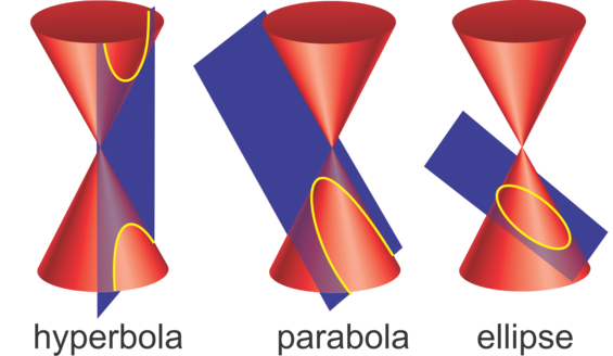
So, creating adjectives from the nouns hyperbola, parabola, and ellipse, we arrive at hyperbolic, parabolic, and elliptic. So far, so good, but what on earth does the plane-cone intersection have to do with our quest to classify PDEs that are relevant for fluid mechanics? Some of you may think: Oh, I know, this looks like the Mach cone, sure, it does, but it has nothing to do with that (or, at least, this is not the reason why we are picking this problem from mathematics to classify our equation).
No, in order to see why this plane-cone intersection is "useful", let us look at the equation that defines this conic section. It is given as
ax^2+bxy+cy^2+dx+ey+f=0
Whenever we are dealing with polynomial equations like the one given above, it is useful to calculate the discriminant. For a polynomial of degree 2, with the form [katex]f(x)=ax^2+bx+c[/katex], it is given as:
\mathrm{Disc}=\Delta=b^2-4acWe can use the same definition of the discriminant for our conic section. The solution of this discriminant will tell us how the roots of the polynomial will behave, and if you look far, far back into your middle school math classes, you may remember the quadratic equation of the form
x_{1,2}=\frac{-b\pm\sqrt{b^2-4ac}}{2a}The discriminant [katex]\Delta[/katex] appears in the root of this quadratic equation, and you may remember that this equation will tell you the intersection of the polynomial [katex]f(x)=ax^2+bx+c[/katex] with the x-axis. You can have either 0, 1, or 2 intersections, depending on the coefficient [katex]a[/katex], [katex]b[/katex], and [katex]c[/katex]. This is shown in the following figure:
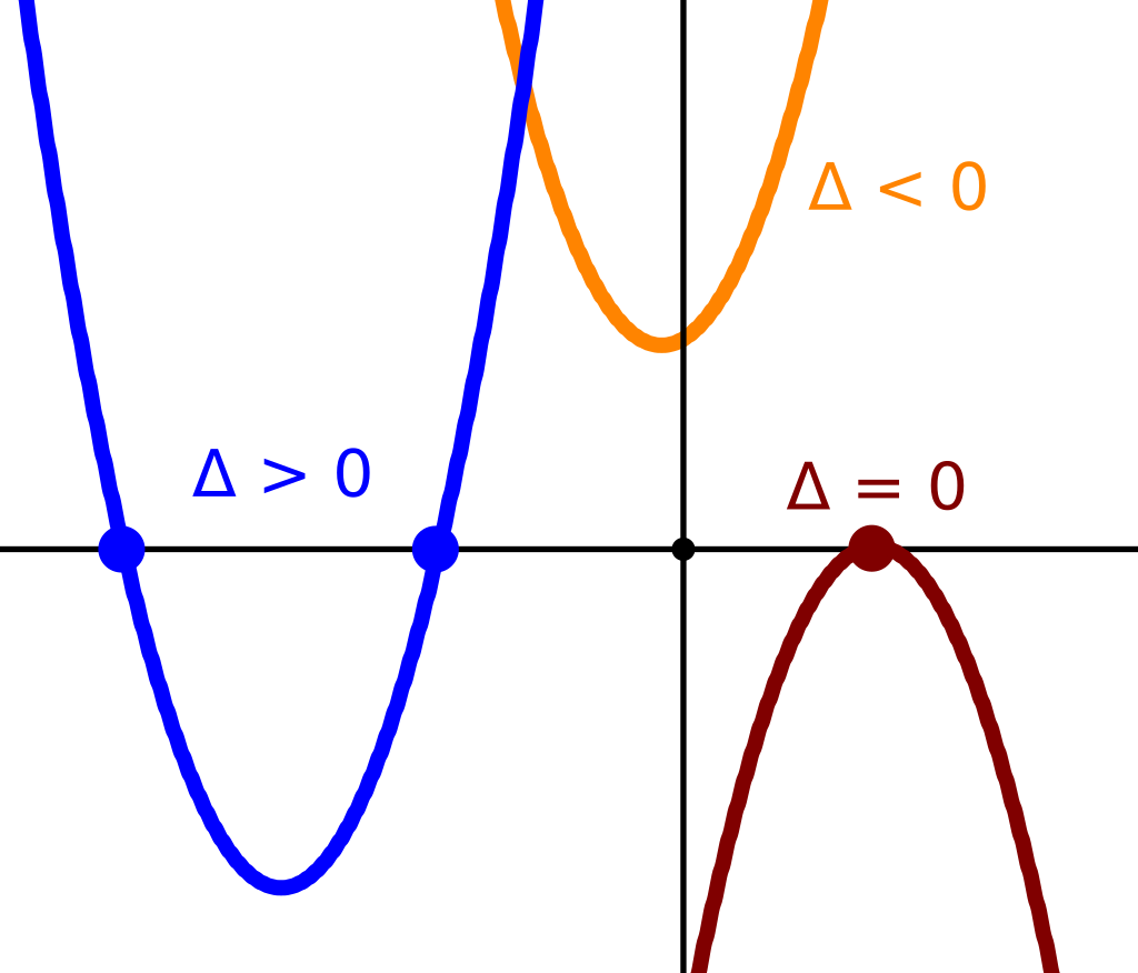
We can now have the following situations:
- [katex]\Delta>0[/katex]: In this case, we have two distinct intersections with the x-axis.
- [katex]\Delta=0[/katex]: In this case, we have one distinct intersection with the x-axis.
- [katex]\Delta<0[/katex]: In this case, there is no distinct intersection with the x-axis.
This concept can now be further extended to the conic section we discussed above. We have the following definition:
- [katex]\Delta>0[/katex]: We obtain a hyperbola.
- [katex]\Delta=0[/katex]: We obtain a parabola.
- [katex]\Delta<0[/katex]: We obtain an ellipse.
So, knowing the conic section equation, and knowing its coefficients, we are able to classify the resulting intersection into either a hyperbola, parabola, or ellipse. So far so good, let's compare that with classifying second-order partial differential equations.
Classifying a second-order partial differential equation into hyperbolic, parabolic, and elliptic form
Let's assume we want to classify an arbitrary second-order PDE. The general equation is of the form:
a\frac{\partial^2 \phi}{\partial x^2}+b\frac{\partial^2 \phi}{\partial x \partial y}+c\frac{\partial^2 \phi}{\partial y^2}+\frac{\partial \phi}{\partial x}+\frac{\partial \phi}{\partial y}+f\phi+g=0Here, we introduced [katex]\phi[/katex] as a general variable, and it could be anything we want (e.g. density, momentum, pressure, temperature, etc.). Let's also introduce another short-hand notation, and let's say we have [katex]X^n=\partial^n/\partial x^n[/katex] and [katex]Y^n=\partial^n/\partial y^n[/katex]. Then, we can rewrite the above equation as
aX^2+bXY+cY^2+dX+eY+f\phi+g=0
Looks familiar? Yes, this is almost identical to our conic section equation, where only the last two terms are different, though they don't play a role in determining the discriminant, i.e. if we were to calculate it for the above equation, we see that both [katex]f[/katex] and [katex]g[/katex] do not play a role in determining the value of the discriminant:
\mathrm{Disc}=\Delta=b^2-4acWe can now introduce the same classification we did above for the discriminant, based on the value it takes:
- [katex]\Delta>0[/katex]: We obtain a hyperbolic equation
- [katex]\Delta=0[/katex]: We obtain a parabolic equation
- [katex]\Delta<0[/katex]: We obtain an elliptic equation
If we go back to the quadratic formula for a moment, i.e.
x_{1,2}=\frac{-b\pm\sqrt{b^2-4ac}}{2a}Then, we can also talk again about the number of solutions for [katex]x[/katex], and we said that we have:
- [katex]\Delta>0[/katex]: We have two distinct intersections with the x-axis.
- [katex]\Delta=0[/katex]: We have one distinct intersection with the x-axis.
- [katex]\Delta<0[/katex]: There is no distinct intersection with the x-axis.
OK, let's return to the somewhat confusing statement that I made at the beginning of this section, where I stated that:
Hyperbolic PDEs have real and distinct characteristics, while parabolic PDEs have real characteristics, which will have the same value. Elliptic PDEs, on the other hand, have only imaginary characteristics.
If we combine the aforementioned properties of the discriminant, quadratic equation, and conic section, we start to understand more of this statement. We now know why we talk about hyperbolic, parabolic, and elliptic equations (at least in the sense of why we have chosen this naming convention).
Hyperbolic PDEs have distinct characteristics (two different roots of the discriminant, i.e. [katex]\Delta>0[/katex]), parabolic PDEs have real characteristics which have the same value (the same root of the discriminant, i.e. [katex]\Delta=0[/katex]), while elliptic equations have no real characteristics, or rather, only imaginary characteristics. Knowing that elliptic equations have [katex]\Delta<0[/katex], if we inserted that into our quadratic equation, we get the square root of a negative number, and hence a complex number with imaginary components.
OK, so this sentence starts to make sense, but it is still somewhat abstract. We will return to this statement later, as we still need to introduce the concept of characteristics more formally, but I want to take the momentum that we have built up now and look into the classification of PDEs that govern CFD applications.
Towards hyperbolic, parabolic, and elliptic equations in fluid dynamics
In this section, we will look at two approaches to classify the governing equation in CFD. The problem is that, when I say governing equations, it can mean anything from linearised potential flow equations to the full, viscous Navier-Stokes equations. Typically, I have found that most textbooks will take an equation which lends itself well for the classification problem, then they classify it, provide some physical meaning, and then move on.
This is great if you have to fill content when you have written 598 pages of your book manuscript but you have contractually agreed to 600 pages with your publisher; it's quick to write, just copy and paste what others have done, and you have augmented your book with some additional insights.
But then the young version of me (during my PhD), or you, comes along and uses that study how to classify the Navier-Stokes equations and we just can't figure out how to apply this approach to the Navier-Stokes equations. Well, it takes a bit more than 2 pages to explain, if only they agreed on 610 pages ...
Let's look then at this simplified approach first, and then afterwards introduce a method that generalises to the Navier-Stokes equations.
The wrong way: The standard CFD textbook approach and why it is wrong
When I first looked into the topic of classifying equations into hyperbolic, parabolic, and elliptic, I looked at various sources (that was over a decade ago now, so it was a bit difficult to track them all down, so I'm working based on what I remember, probably a dangerous proposition ...). They typically provided the definition we saw above, i.e. they start with a second-order partial differential equation and then show that hyperbolic, parabolic, and elliptic equations can be classified based on the value of the discriminant.
I naively applied that to the Navier-Stokes equations, where the non-linear term is no longer of importance (it is only responsible for turbulence, shock waves, boundary layers, 60 different numerical schemes to treat it in OpenFOAM, and pretty much for 75 years of ongoing research into how we can tame it. I suppose it is indeed not of great importance ...), and, if you do that, you start to classify the equation based on the viscous term and get [katex]\Delta=-4\nu^2[/katex], so the Navier-Stokes equation is elliptic. Or is it?
No, this approach does not work here. What the book authors often (pretty much all the time) neglect to say is that the classification of PDEs into hyperbolic, parabolic, and elliptic works really well if we consider steady, adiabatic, two-dimensional, irrotational, and supersonic flow. Well, that seems to me like we are limiting ourselves a bit, but hey, what do I know?
Let's look at this equation, which is given as:
\left(1-\frac{\Phi_x^2}{a^2}\right)\Phi_{xx}-\frac{2\Phi_x\Phi_y}{a^2}\Phi_{xy}+\left(1-\frac{\Phi_y^2}{a^2}\right)\Phi_{yy}=0Essentially, we are dealing with a potential flow here, where I have introduced the following short-hand notation:
\Phi_x=\frac{\partial \Phi}{\partial x}, \quad
\Phi_{xy}=\frac{\partial^2\Phi}{\partial x\partial y}, \quad
\Phi_y=\frac{\partial \Phi}{\partial y}, \quad
\Phi_{xx}=\frac{\partial^2\Phi}{\partial x^2}, \quad
\Phi_{yy}=\frac{\partial^2\Phi}{\partial y^2}
In this context, [katex]\Phi[/katex] is the velocity potential, and we can always obtain the velocity field through the following definition:
u=\Phi_x=\frac{\partial \Phi}{\partial x},\quad v=\Phi_y=\frac{\partial \Phi}{\partial y}Here, we also have the speed of sound defined as [katex]a[/katex]. If we now introduce the definition of the velocity into the brackets of the equation, then we have the following form:
\left(1-\frac{u^2}{a^2}\right)\Phi_{xx}-\frac{2uv}{a^2}\Phi_{xy}+\left(1-\frac{v^2}{a^2}\right)\Phi_{yy}=0Great, let's get busy and classify this equation. We already know how to do it, right? We just calculate the solution of the quadratic formula, and then we classify the equation based on its roots, i.e. the discriminant. Let's do that, then. The quadratic solution to the above equation is given as:
x_{1,2}=\frac{-\frac{2uv}{a^2}\pm\sqrt{\left(\frac{2uv}{a^2}\right)^2-4\left(1-\frac{u^2}{a^2}\right)\left(1-\frac{v^2}{a^2}\right)}}{2\left(1-\frac{u^2}{a^2}\right)}We can now expand the terms inside the square root, which results in the following:
x_{1,2}=\frac{-\frac{2uv}{a^2}\pm\sqrt{\frac{4u^2v^2}{a^4}-4+4\frac{u^2}{a^2}+4\frac{v^2}{a^2}-\frac{4u^2v^2}{a^4}}}{2\left(1-\frac{u^2}{a^2}\right)}The first and fifth terms are the same and opposite in sign, so they cancel out. We can then factorise the second, third, and fourth term to arrive at:
x_{1,2}=\frac{-\frac{2uv}{a^2}\pm\sqrt{4\left(\frac{u^2+v^2}{a^2}-1\right)}}{2\left(1-\frac{u^2}{a^2}\right)}We now introduce the velocity magnitude as [katex]U^2=u^2+v^2[/katex]. If we were to insert that, then we would have [katex]U^2/a^2=M^2[/katex], i.e. the fraction inside the square root is just the square of the Mach number. Inserting this into our equation results in:
x_{1,2}=\frac{-\frac{2uv}{a^2}\pm\sqrt{4\left(M^2-1\right)}}{2\left(1-\frac{u^2}{a^2}\right)}At this point, we could further simplify the equation, but that is beside the point. We are only interested in the discriminant. So, let's see what we have:
- [katex]\Delta=M^2-1>0[/katex]: For this inequality to hold true, we require that [katex]M>1[/katex]. If this is the case, we have a supersonic flow. Since we have [katex]\Delta>0[/katex], the equation is classified as hyperbolic.
- [katex]\Delta=M^2-1=0[/katex]: For this equality to hold true, we require that [katex]M=1[/katex]. If this is the case, we just about reach supersonic flow. Since we have [katex]\Delta=0[/katex], the equation is classified as parabolic.
- [katex]\Delta=M^2-1<0[/katex]: For this inequality to hold true, we require that [katex]M<1[/katex]. If this is the case, we have a subsonic flow. Since we have [katex]\Delta<0[/katex], the equation is classified as elliptic.
You see, using this equation lends itself well to the classification problem. We can derive meaningful flow regimes (i.e. supersonic and subsonic), which nicely correlate with the discriminant. Our publisher is happy that we have crossed the 600 page threshold and our job is done, right? If only we could use potential flow theory for all of our fluid dynamics endeavours, life could be so easy.
So let's then quickly discuss why this approach is rubbish. The first and most obvious point is that life is not steady-state, adiabatic, irrotational, two-dimensional, and supersonic. The general Navier-Stokes equations are unsteady, allow for heat transfer, rotational, three-dimensional, and work for subsonic and supersonic, incompressible and compressible, laminar and turbulent flows alike!
But that's not all. The Navier-Stokes equations are a system of equations. Imagine the continuity equation for an incompressible flow; it is given as:
\nabla\cdot\mathbf{u}=\frac{\partial u}{\partial x}+\frac{\partial v}{\partial y}+\frac{\partial w}{\partial z}=0Good luck classifying that with your second-order PDE approach. Using the discriminant approach here would result in [katex]\Delta=0[/katex], but as we will see later, the continuity equation is responsible for making our system either fully hyperbolic or mixed elliptic-hyperbolic!
So, while we can use the approach outlined in the second-order PDE section for our simplified supersonic potential flow equation, it just doesn't generalise to the more complex Navier-Stokes equations. But, the longer I do CFD, the more I get the feeling that authors of textbooks do not read sufficient background information to confidently write about a topic but instead copy of what is out there.
Take the book of Versteeg and Malalsekera, one of my favourite introductory textbook out there. If you read this first and then you look at the textbook of Patankar (and I've read both cover to cover), then you wonder how Versteeg and Malalasekera got away with this blatant plagiarism. Sure, the text is different, but the initial chapters follow exactly the same ideas, equations, and examples.
CFD textbook authors are lazy, and if you ever feel reading any of these books is over your head and you don't understand what they are talking about, it is because they are lazy and didn't take the time to explain things properly, not because you aren't clever enough! When I started with CFD, I constantly felt challenged by my CFD books. It can't just be me ...
Anyway, rant-time is over. Let's now turn to an approach I have found to work great for classifying PDEs that are of interest for CFD applications and extend to all different kinds of governing equations.
The right way: the Hellwig-Hoffmann-Chiang approach (I love you guys!). Alright, Anderson, you can join the party as well!
The best approach to classify PDEs into hyperbolic, parabolic, and elliptic equations is given by Hoffmann and Chiang (see my reading list for details). Their approach is based on the work of Hellwig and does a bit of the opposite of what we have looked at above. Anderson does introduce a similar, generalised approach in his book but doesn't bother specifying how it would work for mixed systems, but then again I suppose his book is from a time when Euler equations were still dominating (i.e. a system of pure first-order PDEs).
These three authors show that we can classify a system of equations, which is good for us, as we want to classify the continuity and momentum equation, at a minimum, to tell us the type of our solution. However, they also make one simplification (and provide a solution to overcome this; at least in the book of Hoffmann and Chiang, Anderson does not show this).
The simplification is that we are now classifying a system of first-order PDEs. Any second order term is simply dropped, similar to what we did when we looked at the classification of a second-order PDE above. This is, however, not a big deal; Hoffmann and Chiang show how we can extend this approach to a mixed system of first and second order PDEs, but the result remains the same. So, for our intent and purposes, limiting ourselves to first-order PDEs is actually not a limitation.
So how does this approach work? Well, it works in 1D, 2D, and 3D, though it doesn't really matter which approach we take. 1D is pretty simple and straight forward and does not require fancy dimension-merging techniques, but 2D does. 3D is an extension of the 2D dimension merging approach, but results in the same, albeit more difficult to interpret results, so we will look at 2D results here first.
We'll do the classification twice, once for the time-dependent (unsteady) and time-independent (steady-state) flow. We'll see how this time-dependence will be crucial in determining the type. We will also do the classification based on incompressible flows, which makes life a bit more difficult for us compared to compressible flows. If you understand the incompressible case, compressible flows are easy to classify but not vice versa.
Classifying time-independent (steady-state), incompressible flows
The full Navier-Stokes equations for a 2D, incompressible flow can be given as
- Continuity equation:
\frac{\partial u}{\partial x}+\frac{\partial v}{\partial y}=0- Momentum equation in X:
u\frac{\partial u}{\partial x} + v\frac{\partial u}{\partial y} =
-\frac{1}{\rho}\frac{\partial p}{\partial x}+\nu\frac{\partial^2 u}{\partial
x^2} + \nu\frac{\partial^2 u}{\partial y^2}- Momentum equation in Y:
u\frac{\partial v}{\partial x} + v\frac{\partial v}{\partial y} =
-\frac{1}{\rho}\frac{\partial p}{\partial y}+\nu\frac{\partial^2 v}{\partial
	x^2} + \nu\frac{\partial^2 v}{\partial y^2}
In order to classify these equation, we want to write them in a compact matrix coefficient form, which allows us to calculate the properties of the matrix which we can related to the character of the flow. This may sound confusing for now, but hang on for a moment, it'll become clear in a second.
We start by recasting the above three equations into a matrix form like so:
\mathbf{\mathcal{A}}\frac{\partial \mathbf{Q}}{\partial x} +
\mathbf{\mathcal{B}}\frac{\partial \mathbf{Q}}{\partial y} = 0
Here, we have [katex]\mathcal{A}[/katex] and [katex]\mathcal{B}[/katex] representing our coefficient matrices in the [katex]x[/katex] and [katex]y[/katex] direction, while [katex]\mathbf{Q}[/katex] represents the conserved flow variables in our system. These two matrices and one vector are given as:
\mathbf{\mathcal{A}} =
\begin{bmatrix}
1 & 0 & 0\\
u & 0 & \frac{1}{\rho}\\
0 & u & 0
\end{bmatrix}, \quad
\mathbf{\mathcal{B}} =
\begin{bmatrix}
0 & 1 & 0\\
v & 0 & 0\\
0 & v & \frac{1}{\rho}
\end{bmatrix}, \quad
\mathbf{Q} =
\begin{bmatrix}
u\\
v \\
p
\end{bmatrix}
Let's look at how these came about. Each row in the matrices represents one equation; the first row is the continuity equation, the second is the momentum equation in x, and the third and last row is the momentum equation in y. If we multiply the first row in [katex]\mathcal{A}[/katex] with [katex]\mathbf{Q}[/katex], then we obtain [katex]1\cdot u + 0 \cdot v + 0 \cdot p = u[/katex]. Similarly, if we do that for the [katex]\mathcal{B}[/katex] matrix, we get [katex]0 \cdot u + 1 \cdot u + 0 \cdot p = v[/katex]. If we insert these two values now in the above equation, then we get [katex]\partial u/\partial x + \partial v/\partial y=0[/katex].
Go ahead and do that for rows two and three if you don't trust me, and you'll see that we obtain the momentum equations again. You'll notice that the second-order derivatives are now gone. This is the simplification I mentioned above, i.e. we focus here now on the system of first order derivatives. Stick around for a bit longer, and I'll show you how you can re-introduce the second-order derivatives, though it wouldn't change anything about our classification, as mentioned earlier.
So, we now have two coefficient matrices, and our goal is to derive some form of meaning about the flow from these matrices. In physics, whenever we want to interrogate the behaviour of a system that is represented in matrix form, we look at eigenvalues and eigenvectors that, for different systems, will have specific meanings. It turns out that, in our case, the eigenvalues can be used to classify the system into hyperbolic, parabolic, and elliptic flows.
For the moment, we just have to accept this fact, but I will show you later why this works and what these eigenvalues physically represent. But before we can go ahead and calculate eigenvalues, we have to face the issue of having two matrices (see, this is what I meant with 1D is easy, where we would only have one matrix now). We have to combine both matrices, so Hellwig, Hoffman, and Chiang proposed multiplying each matrix with the unit normal vector of the direction they represent.
The [katex]\mathcal{A}[/katex] matrix represents derivatives in the [katex]x[/katex] direction, and so we multiply it by [katex]n_x[/katex]. Similarly, we multiply [katex]\mathcal{B}[/katex] by the normal vector in the [katex]y[/katex] direction, which provides us with a new, combined matrix [katex]\mathcal{T}[/katex] as:
\mathbf{\mathcal{T}} = \mathbf{\mathcal{A}}\cdot n_x + \mathbf{\mathcal{B}}\cdot
n_y
Doing this allows us to retain the information of what component contributes to the [katex]x[/katex] and [katex]y[/katex] direction, while the addition in the above equation results in a single matrix. We can then compute the eigenvalues of this single matrix, providing us with a means to classify our equations.
Let's construct [katex]\mathcal{T}[/katex] first, carrying out the multiplication and addition shown above results in:
\mathbf{\mathcal{T}} =
\begin{bmatrix}
n_x & n_y & 0 \\
u n_x + v n_y & 0 & \frac{n_x}{\rho} \\
0 & u n_x + v n_y & \frac{n_y}{\rho}
\end{bmatrix}
We are now in a position to calculate the eigenvalues of this equation. We do that by calculating the determinant of [katex]\mathcal{T}[/katex]. This is done as shown in the following:
\mathrm{det}(\mathbf{\mathcal{T}})=+\frac{n_x^2}{\rho}(u n_x + v
n_y)+\frac{n_y^2}{\rho}(u n_x + v n_y) = 0
Let's clean this up a little bit. First, we'll multiply by [katex]\rho[/katex], and then we'll get rid of the parenthesis, which results in:
u n_x^3 + v n_x^2 n_y + u n_x n_y^2 + v n_y^3 = 0
OK, we have these mixed normal vector components in our system, which we want to get rid of somehow. First, we will divide the equation by [katex]n_x^3[/katex]. This results in:
u+v\frac{n_y}{n_x}+u\frac{n_y^2}{n_x^2}+v\frac{n_y^3}{n_x^3}=0If we now introduce the short-hand notation [katex]x=n_y/n_x[/katex], we can write the above equation (in rearranged form) as:
v x^3 + u x^2 + v x + u = 0
Look familiar? Yes, we have arrived again at a polynomial equation, but this time only dependent on [katex]x[/katex], and also, this is a third-order polynomial, meaning there are three possible roots to this equation. You could use something like factorisation of a cubic equation to get to this solution, but you may as well also use software such as Maple, Matlab, or Python. Either way, these are the three solutions you should arrive at:
x_1 = +\sqrt{-1}, \qquad x_2=-\sqrt{-1}, \qquad x_3=-\frac{u}{v}We have two imaginary solution ([katex]x_1[/katex] and [katex]x_2[/katex]), while [katex]x_3[/katex] provides a real eigenvalue. As a result, the system of equations for the incompressible Navier-Stokes equation is classified as mixed elliptic-hyperbolic. Why hyperbolic? Well, we have real and distinct eigenvalues (in this case, only one), which makes it hyperbolic. But why not mixed elliptic-parabolic?
In my view, both classifications would be correct as long as we ignore the imaginary part. If we want to be strict, though, a parabolic equation requires all eigenvalues to be the same (and real), which they are not in this case. But then again, you could make the argument as well that hyperbolic doesn't make any sense, as the eigenvalues are also not real and distinct.
It is a convention struck in the literature, and we may as well just follow it (knowing full well that most authors who claim the equations to be mixed elliptic-hyperbolic have likely never done the classification themselves on paper!)
But I hope this illustrates how to classify a system of first-order PDEs. Next, we'll do the same for time-dependent flows.
Classifying time-dependent (unsteady), incompressible flows
In this section, we'll go through the same steps and see how the time-dependent nature of the Navier-Stokes equation changes things. I'll be brief on the derivation, as it largely follows the same steps as above, but I want to spend some time looking at what is causing the differences and then provide some physical intuition as to why this makes sense.
We start again with the system of the 2D, incompressible, unsteady Navier-Stokes equations, which now become:
- Continuity equation:
\alpha \frac{\partial p}{\partial t}+\frac{\partial u}{\partial x}+\frac{\partial v}{\partial y}=0- Momentum equation in X:
\frac{\partial u}{\partial t}+u\frac{\partial u}{\partial x} + v\frac{\partial u}{\partial y} =
-\frac{1}{\rho}\frac{\partial p}{\partial x}+\nu\frac{\partial^2 u}{\partial
x^2} + \nu\frac{\partial^2 u}{\partial y^2}- Momentum equation in Y:
\frac{\partial v}{\partial t}+u\frac{\partial v}{\partial x} + v\frac{\partial v}{\partial y} =
-\frac{1}{\rho}\frac{\partial p}{\partial y}+\nu\frac{\partial^2 v}{\partial
	x^2} + \nu\frac{\partial^2 v}{\partial y^2}
Here, we used a little trick, and this is where I mentioned earlier that classifying the incompressible Navier-Stokes equations is a bit trickier than the compressible version. The trick here is how we introduce the time dependence into the continuity equation. For a compressible flow, we have the continuity equation as
\frac{\partial \rho}{\partial t}+\frac{\partial \rho u}{\partial x}+\frac{\partial \rho v}{\partial y}=0Our trick here is to say that the pressure and density are related through some equation. For compressible flows, this would be, for example, the ideal gas law, but of course, for incompressible flows, this does not hold. So, instead, we say that we have some form of functional relationship that can be expressed as [katex]\rho=\alpha p[/katex].
From a physical point of view, this may be regarded as questionable, but in practice this works well. If we look, for example, at the artificial compressibility method, this is exactly what we do, and for the purpose of classifying our equations, this works out really well. The reason why we want to express the density as a pressure is because of the vector [katex]\mathbf{Q}[/katex], which, if you recall, was defined as [katex]\mathbf{Q}=[u,v,p]^T[/katex].
We want to express all of our derivatives in terms of the entries in our [katex]\mathbf{Q}[/katex] vector, and since there is no density, we want to express this as a pressure instead. With this substitution done, we can now go ahead and form our system again as
\mathbf{\mathcal{A}}\frac{\partial \mathbf{Q}}{\partial t} +
\mathbf{\mathcal{B}}\frac{\partial \mathbf{Q}}{\partial x} +
\mathbf{\mathcal{C}}\frac{\partial \mathbf{Q}}{\partial y} = 0
Now, we also have a matrix for the time derivatives, which spices things up a bit. So, we have three matrices in total. We can define these three matrices as:
\mathbf{\mathcal{A}} =
\begin{bmatrix}
0 & 0 & \alpha \\
1 & 0 & 0 \\
0 & 1 & 0
\end{bmatrix}
,\quad
\mathbf{\mathcal{B}} =
\begin{bmatrix}
1 & 0 & 0\\
u & 0 & \frac{1}{\rho}\\
0 & u & 0
\end{bmatrix}
,\quad
\mathbf{\mathcal{C}} =
\begin{bmatrix}
0 & 1 & 0\\
v & 0 & 0\\
0 & v & \frac{1}{\rho}
\end{bmatrix},\quad
\mathbf{Q} =
\begin{bmatrix}
u\\
v \\
p
\end{bmatrix}
The definition for [katex]\mathbf{Q}[/katex] remains the same, as you can see. We now introduce the new combined coefficient matrix as:
\mathbf{\mathcal{T}} = \mathbf{\mathcal{A}}\cdot n_t + \mathbf{\mathcal{B}}\cdot
n_x + \mathbf{\mathcal{C}}\cdot n_y
I have introduced a new normal vector component, which is now defined in time as [katex]n_t[/katex]. This normal vector points in the direction of time, which, I agree, in the context of normal vectors is perhaps a bit confusing, but this direction is constructed simply in analogy to how we defined [katex]n_x[/katex] and [katex]n_y[/katex]. Carrying out the multiplication and addition results in
\mathbf{\mathcal{T}} =
\begin{bmatrix}
n_x & n_y &  \alpha n_t\\
n_t + u n_x + v n_y & 0 & \frac{n_x}{\rho} \\
0 & n_t + u n_x + v n_y & \frac{n_y}{\rho}
\end{bmatrix}
In order to classify this new combined coefficient matrix, we do the same as we did before, i.e. we calculate the determinant and set the right-hand side to zero to obtain the type of flow. This is shown in the following:
\mathrm{det}(\mathbf{\mathcal{T}}) = \alpha n_t(n_t + u n_x + v n_y)^2 -
\frac{n_x^2}{\rho}(n_t + u n_x + v n_y) - \frac{n_y^2}{\rho}(n_t + u n_x + v
n_y) = 0
We can expand this equation (multiply out the parenthesis) to arrive at the following form:
-\rho\alpha (n_t^3 + 2 u n_t^2 n_x + 2 v n_t^2 n_y + 2 u v n_x n_y n_t + u^2 n_t
n_x^2 + v^2 n_t n_y^2) + n_x^2 n_t + u n_x^3 + v n_y n_x^2 + n_y^2 n_t +u n_x n_y^2 + v n_y^3 = 0
Hmmm, OK, so this looks a bit more challenging all of a sudden. Now, we have to deal with three dimensions, i.e. [katex]n_t[/katex], [katex]n_x[/katex], and [katex]n_y[/katex]. We can't simply divide by one normal direction and then express the equation in a convenient polynomial as we did before, but we can modify the equation that will allow us to do just that.
We can use the fact that the Navier-Stokes equations are Galilean invariant, which in this context simply means that the equations do not change from one coordinate direction into another (if we rotate the coordinate system around one axis, the equations would still be the same).
This means that we can split the equations in the [katex]x[/katex] and [katex]y[/katex] direction and this is exactly how we proceed with the above equation. We will construct two equations; one for the [katex]n_t[/katex] and [katex]n_x[/katex] space, and one for the [katex]n_t[/katex] and [katex]n_y[/katex] space. These two equations can be obtained as:
- [katex]n_t[/katex] and [katex]n_x[/katex] space
-\rho\alpha (n_t^3 + 2 u n_t^2 n_x + u^2 n_t n_x^2) + n_x^2 n_t + u n_x^3 = 0
- [katex]n_t[/katex] and [katex]n_y[/katex] space
-\rho\alpha (n_t^3 + 2 v n_t^2 n_y + v^2 n_t n_y^2) + n_y^2 n_t + v n_y^3 = 0
We can now classify either of these equations and, since these equations are Galilean invariant, we will arrive at the same classification, regardless of which equation we choose.
Now, we can proceed in a similar way as we did before. Looking at the equation in [katex]n_t[/katex] and [katex]n_x[/katex] space first, we divide the equation by [katex]\rho\alpha[/katex], as well as [katex]n_t^3[/katex], and we introduce the substitution of [katex]x=n_x/n_t[/katex]. Then, we arrive at
\frac{u}{\rho\alpha} x^3 + \left(\frac{1}{\rho\alpha}-u^2\right)x^2 - 2 u x - 1 = 0We can do the same in the [katex][/katex] direction, where we divide the equation by [katex]n_t[/katex] and introduce the short-hand notation [katex]y=n_y/n_t[/katex]. This leads to:
\frac{v}{\rho\alpha} y^3 + \left(\frac{1}{\rho\alpha} - v^2\right)y^2 - 2 v y - 1 = 0Finding the roots of the cubic equations results in the following solutions in the x-direction:
x_1=-\frac{1}{u}, \qquad x_2 =
\frac{u\rho\alpha}{2}+\frac{\rho\alpha}{2}\sqrt{\frac{u^2\rho\alpha+4}{\rho\alpha}},
\qquad x_3 = \frac{u\rho\alpha}{2}-\frac{\rho\alpha}{2}\sqrt{\frac{u^2\rho\alpha+4}{\rho\alpha}}
Similarly, in the y-direction, we have the following solutions:
y_1=-\frac{1}{v}, \qquad y_2 =
\frac{v\rho\alpha}{2}+\frac{\rho\alpha}{2}\sqrt{\frac{v^2\rho\alpha+4}{\rho\alpha}},
\qquad y_3 = \frac{v\rho\alpha}{2}-\frac{\rho\alpha}{2}\sqrt{\frac{v^2\rho\alpha+4}{\rho\alpha}}
Before we can classify the system, let us look into the square roots. In the [katex]n_t[/katex] and [katex]n_x[/katex] space, we have
\sqrt{\frac{u^2\rho\alpha+4}{\rho\alpha}}Since the velocity is squared, no matter what its value or sign, it will always be a positive number. The density is also always positive, while [katex]\alpha[/katex] is assumed to be also positive, as it is a functional relationship of other thermodynamic properties such as the gas constant and temperature. Thus, no matter the values, the root will always contain a positive number. Since no negative numbers can occur here, we won't get complex numbers.
Thus, we can say that all eigenvalues are real and distinct, and as a result, we classify the time-dependent Navier-Stokes equations as fully hyperbolic.
Remember that we introduced this little trick to introduce the time derivative in the Navier-Stokes equation artificially. Let's take the pure incompressible Navier-Stokes equation, where we do not have a time derivative in the continuity equation. You won't get a hyperbolic system but a mixed elliptic-hyperbolic system again instead.
Similarly, if we take the pure compressible Navier-Stokes equation, we have the time dependence on the density in the continuity equation, i.e.
\frac{\partial \rho}{\partial t}+\nabla\cdot(\rho\mathbf{u})=0This time dependence turns the compressible Navier-Stokes equations hyperbolic. To see that, we need to write down the determinant, and we'll observe that the absence of the time derivative will introduce imaginary components in the solutions to our cubic equation.
Classifying mixed systems of first- and second-order derivatives
OK, so what happens then if you have to deal with the full system of the Navier-Stokes equations? This section will outline this step, but the derivation is long, and it will arrive at the same result. The most tricky bit is getting the equations right. Once that is done, developing the determinant takes some time, which again, can (or probably should) be done using some sort of symbolic math library, be it Maple (my favourite for these types of tasks!), Matlab (meh), or Python (you just have an answer/package for everything, don't you?!).
Let's start out by writing the system down first. Looking at a steady-state, incompressible flow again, we have:
- Continuity equation:
\frac{\partial u}{\partial x}+\frac{\partial v}{\partial y}=0- Momentum equation in X:
u\frac{\partial u}{\partial x} + v\frac{\partial u}{\partial y} =
-\frac{1}{\rho}\frac{\partial p}{\partial x}+\nu\frac{\partial^2 u}{\partial
x^2} + \nu\frac{\partial^2 u}{\partial y^2}- Momentum equation in Y:
u\frac{\partial v}{\partial x} + v\frac{\partial v}{\partial y} =
-\frac{1}{\rho}\frac{\partial p}{\partial y}+\nu\frac{\partial^2 v}{\partial
	x^2} + \nu\frac{\partial^2 v}{\partial y^2}
The trick is now to express second-order derivatives as first-order derivatives so that we have a system of first-order derivatives again. We can achieve that by introducing the following four new equations:
a=\frac{\partial u}{\partial x},\quad b=\frac{\partial u}{\partial y},\quad c=\frac{\partial v}{\partial x},\quad d=\frac{\partial v}{\partial y}With these introduced, the Navier-Stokes equations now become:
- Continuity equation:
\frac{\partial u}{\partial x}+\frac{\partial v}{\partial y}=0- Momentum equation in X:
u\frac{\partial u}{\partial x} + v\frac{\partial u}{\partial y} =
-\frac{1}{\rho}\frac{\partial p}{\partial x}+\nu\frac{\partial a}{\partial
x} + \nu\frac{\partial b}{\partial y}- Momentum equation in Y:
u\frac{\partial v}{\partial x} + v\frac{\partial v}{\partial y} =
-\frac{1}{\rho}\frac{\partial p}{\partial y}+\nu\frac{\partial c}{\partial
	x} + \nu\frac{\partial d}{\partial y}
Our solution vector [katex]\mathbf{Q}[/katex] now becomes [katex]\mathbf{Q}=[a, b, c, d, u, v, p]^T[/katex] and the corresponding system of equations
\mathbf{\mathcal{A}}\frac{\partial \mathbf{Q}}{\partial x} +
\mathbf{\mathcal{B}}\frac{\partial \mathbf{Q}}{\partial y} = \mathcal{C}
At this point, we write out equations for [katex]\mathcal{A}[/katex] and [katex]\mathcal{B}[/katex]. Since [katex]\mathbf{Q}[/katex] now contains seven entries, our matrices must also contain seven rows and columns (in order to calculate the determinant, it must be a square matrix). The trick becomes in defining the additional four equations through some combinations of [katex]a, b, c, d[/katex] using the continuity equation. Hoffmann and Chiang provide an idea for how to construct such equations.
Furthermore, we now also have a right-hand side vector [katex]\mathcal{C}[/katex], which allows us to have non-zero values on the right-hand side. With these additional equations in place, we can now construct our combined matrix [katex]\mathcal{T}[/katex] as before:
\mathbf{\mathcal{T}} = \mathbf{\mathcal{A}}\cdot n_x + \mathbf{\mathcal{B}}\cdot
n_y
This will now be a seven-by-seven matrix, of which you have to calculate the determinant. You probably don't want to do this yourself, but again, use a program that can do that for you. Then, you set the determinant equal to zero, i.e. [katex]\mathrm{det}(\mathcal{T})=0[/katex], solve for [katex]x=n_y/n_x[/katex], and depending on the solution of [katex]x[/katex], you can now classify your system as hyperbolic, parabolic, and elliptic. The values may be different to the solution we saw above, but the behaviour should still remain the same.
So what gives? What do hyperbolic, parabolic, and elliptic equations physically represent
So, we have spend now quite a bit talking about hyperbolic, parabolic, and elliptic equations, but what's the point of doing this? Of course, we can calculate mathematical properties all day long, but without a reason, this becomes a futile exercise. So why do we care about the mathematical character of an equation?
Simply put, the character of the equation will determine the solution algorithms we use to solve the underlying equations. Elliptic equations require a wildly different solution approach than hyperbolic equations, while parabolic equations, perhaps, sit in between the two. Thus, we need to know the mathematical character of our equations first before we can select any numerical schemes and algorithms to solve them.
But before we jump into the different types, I want to touch upon a topic yuou can't avoid when talking about hyperbolic, parabolic, and elliptic equations; characterisitcs. This is another often quoted fluid mechanic property which I find seldomly explained well, and that is because it can have several definitions based on the context.
I'll do my best to explain to you the two types of characteristics that exists first (which really are just one type, but it is easier to understand them if we treat them as separate entities for the moment) and then we'll finally take a look at hyperbolic, parabolic, and elliptic flows.
Precursor: The method of characteristics
As alluded to above, there are two ways to explain the method of characterisitcs. We'll look at both of them and then bring both explanations together. Let's start with the first.
Type 1 characteristics
To understand these characteristics, let's look at a classic example: the (Sod) shock tube problem. If you start out writing your own compressible Euler solver, then you'll likely start implementing the shock tube problem first. It is a great example as you have to deal with discontinuities (which are a pain to capture using numerical schemes) while you can keep the complexity low, as it works just as well in 1D, as it does in 2D and 3D.
The basic setup is as follows: You have a tube which has a separator in the centre. This separator splits the tube into a high and low-pressure zone. Once the separator is removed, a shock wave will form and travel to the right (low-pressure region). As a result, we will get a shock wave, a contact discontinuity, and a rarefaction fan. This is shown in the simulation animation below:
Suppose we concentrate our attention on the density plot (top left). In that case, we can create the following schematic representation, where the first three plots simply show the solution of the density profile at three separate time instances.
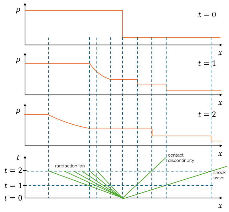
We can see that the rarefaction fan is travelling to the left, while the contact discontinuity and shock wave are travelling to the right. So, let's make sense of all of these blue construction lines that I drew (I went a bit wild!).
What we are trying to do here is to track characteristic points in our flow. Let's look at the solution at [katex]t=0[/katex]. Here, we could say there is only one characteristic point, and that is the discontinuity at the centerline. However, as we progress the solution in time, say at [katex]t=1[/katex], we can see a clear development of a contact discontinuity and a shock wave. These two waves are travelling at a certain speed, and we can see that they have travelled further to the right at [katex]t=2[/katex].
Now what happens if we track these points in time (i.e. the wave front if you want). This is shown in the bottom plot. Here, we plot how our characteristic lines develop over space and time. On the y-axis, we can see that we are now plotting the solution over time instead of [katex]\rho[/katex]. We go into each plot of [katex]\rho[/katex] at various times, track where our contact discontinuity and shock wave are, and then plot their location, in space and time, in the bottom plot.
For example, concentrating on the contact discontinuity for now, it does not show at [katex]t=0[/katex], and from the video, we can see it develops from the center of the domain, hence in the bottom plot, it is located in the center at [katex]t=0[/katex]. Then, at some time [katex]t=1[/katex], it has travelled to the right. We note the location in [katex]x[/katex] and plot that in the bottom plot at the corresponding time level [katex]t=1[/katex]. We can do that for time level [katex]t=2[/katex] as well and see that we get a linear line.
We can continue to do so for the shock wave as well and get a similar result. For the rarefaction fan, since we can find an arbitrary number of characteristics (say, at a specific value for [katex]\rho[/katex]), we get an arbitrary number of characteristics. This is typically visualised by a few lines, but in reality, we would have infinitely many lines.
Using this description, we can say that characteristics track physically relevant properties in space and time (e.g. shock waves, pressure waves more generally, a temperature front, multiphase interphase, etc.).
Type 2 characteristics
The second explanation you will often find in a textbook is related to characteristic curves that we can define mathematically. Let's look at our cubic equation again that we found earlier when classifying our PDEs (see how it all comes together nicely now?!):
u+v\frac{n_y}{n_x}+u\frac{n_y^2}{n_x^2}+v\frac{n_y^3}{n_x^3}=0Here, we have used [katex]n_x[/katex] and [katex]n_y[/katex] to specify the flow going in the [katex]x[/katex] or [katex]y[/katex] direction, respectively. What happens if we make this normal vector component arbitrarily small? Well, we get:
\frac{n_y}{n_x}\rightarrow \frac{\mathrm{d}y}{\mathrm{d}x}Similarly, we can also define the following differential operators:
\frac{n_x}{n_t}\rightarrow \frac{\mathrm{d}x}{\mathrm{d}t},\quad \frac{n_y}{n_t}\rightarrow \frac{\mathrm{d}y}{\mathrm{d}t}Look familiar? What do these represent? Well, let's look at a simple example:
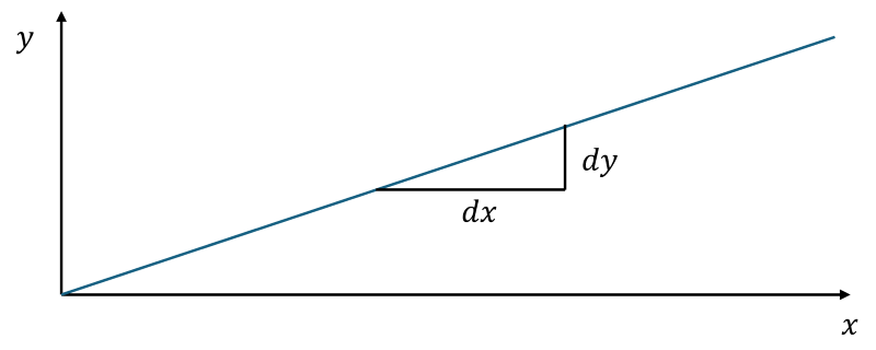
Here, we are just looking at a linear line with a constant slope. To determine the slope, we have to look at the slope over a small distance, which can be determined as [katex]\mathrm{d}y/\mathrm{d}x[/katex]. Thus, if we want to introduce characteristics this way, then we could say that characteristics are simply the slope within a plane at any given point. We saw above that we can track these characteristics in time to visualise them.
In fact, in our definition of the first type of characteristics, what did we see? Our characteristics were defined in the [katex]x,t[/katex] space. In other words, we can define our characteristics as [katex]n_x/n_t\rightarrow\mathrm{d}x/\mathrm{d}t[/katex]! Types 1 and 2 are really just the same, but they are commonly introduced (and treated) differently. Hopefully, this will give you a better, unified view of what characteristics are!
I should mention at this point that I limited myself here to characteristics we could visually see in the flow, but characteristics do exist at each point in the flow. They may just not be as easily visible as, for example, shock waves. Take the case of the rarefaction fan. In this case, we were drawing several (in fact, infinitely many) characteristics emanating from the origin and travelling backwards.
If you want to get a visual intuition, imagine a particle travelling with the flow. Tracking this particle in time, not in space, will give you the trajectory along the characteristic. If the particle is sitting on top of a shock wave, and you were to plot its trajectory in the [katex]x,t[/katex] space, then you would get exactly the same plot as we saw above, where we tracked the shock wave, contact discontinuity, and rarefaction fan.
You could argue, then, that characteristics are just streamlines in time (not space), though this isn't a mainstream view on the matter. But if it helps you grasp the concept of characteristics, then this analogy is a good approximation of what characteristics are.
We have introduced the notion of characteristics now, but what have we gained? Not much, yet! We need to talk about hyperbolic, parabolic, and elliptic flows again and introduce the concept of characteristics. Once we talk about both concepts in conjunction, we will finally start to put all the pieces together and get an intuition for what these different types represent.
Hyperbolic flows
First up, let us discuss hyperbolic flows. We said that hyperbolic equations have the properties of having real and distinct eigenvalues. But what does this eigenvalue physically represent? Well, it is very closely correlated to the characteristics I introduced above. If you go to any point in the flow, you will be able to compute two or more distinct eigenvalues or characteristics, and if they are real, that means you can see them in your flow.
Take the case of a supersonic flow around a diamond-shaped airfoil. This is shown below, both for a simulation on the left and schematically on the right.
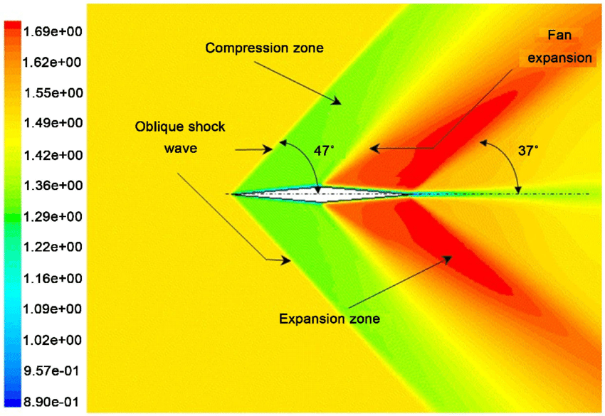
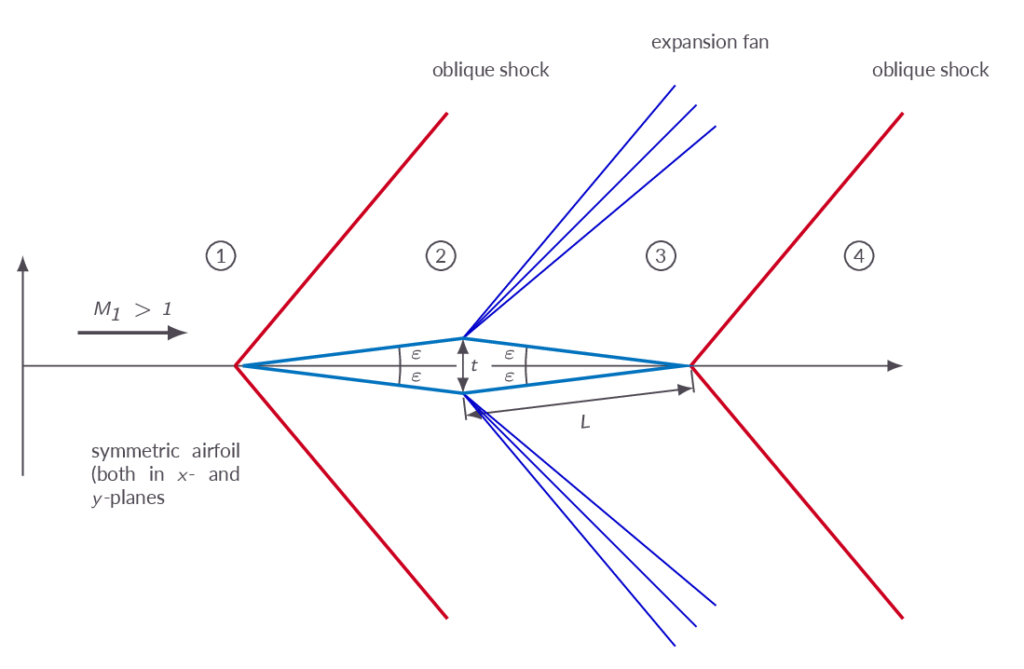
If we concentrate on the leading edge, for the moment, then we can see that we generate two shock waves, one travelling past the upper surface and another one travelling past the bottom surface. Similarly, we can another pair of shock waves at the trailing edge, as well as an expansion fan at the convex corners of the airfoil. Thus, we can visibly see distinct characteristics emanating from a single point.
If we classify the compressible Navier-Stokes equations, they turn out to be purely hyperbolic in nature, thus allowing for multiple shockwaves at a single point to be created, and this hyperbolic behaviour is thanks to the time-dependence of the density in the continuity equation, i.e.
\frac{\partial \rho}{\partial t}+\nabla\cdot(\rho\mathbf{u})=0Compare that to the continuity equation for an incompressible flow
\nabla\cdot\mathbf{u}=0The time derivative is missing here, and if you carry out the classification as presented above, you'll see that the loss of the time derivative in the continuity equation is responsible for the mixed elliptic nature of the system, as alluded to also earlier.
It also explains a lot about the artificial compressibility method. This method was introduced to solve incompressible flows, but taking inspiration from the compressible Navier-Stokes equations. It is the artificial compressibility method because it mimics the compressible Navier-Stokes equations, especially for the continuity equation, which we saw above to be
\frac{1}{\beta}\frac{\partial p}{\partial \tau}+\nabla\cdot\mathbf{u}=0I have replaced [katex]\beta^-1=\alpha[/katex] here, as this is the common notation in the literature, and also introduced the artificial, or pseudo time [katex]\tau[/katex], which indicates that this time derivative is in pseudo time and thus not physically correct. However, this time derivative provides us with a means to solve this equation for the pressure, i.e.
\frac{1}{\beta}\frac{p^{n+1}-p^n}{\Delta \tau}+\nabla\cdot\mathbf{u}=0This can be rearranged to read:
p^{n+1} = p^n-\Delta \tau\beta\nabla\cdot(\mathbf{u})=0Thus, we have an easy mechanism to compute the pressure, which can then be inserted into the momentum equation, and we have found a way to couple pressure and velocity again, which is the main challenge for incompressible flows.
Since we do introduce the time derivative again in the continuity equation, the artificial compressibility method becomes hyperbolic again, and thus allows the usage of numerical schemes that are design for purely hyperbolic flows. What are these methods and schemes?
Well, it turns out that your eigenvalues are related to the speed of sound. So, for each point in your numerical grid, you can calculate your eigenvalues and determine if your flow, at that point, is locally subsonic, transonic, or supersonic. Why is that important? Well, if it is subsonic, we know that there won't be any shock waves, but for supersonic, we may reasonably expect that these could be present, and so we may want to treat them differently. We can thus tailor the way we approximate fluxes based on the nature of the flow.
This is what Riemann solvers do. I am overly simplifying here for the sake of grasping the concepts, but a Riemann solver will essentially use information that is locally available, that relates to the eigenvalues, and use that to compute fluxes based on this local, physical information. Riemann solvers are used to solve the Riemann problem. What is the Riemann problem? The solution across a discontinuity, as shown below:
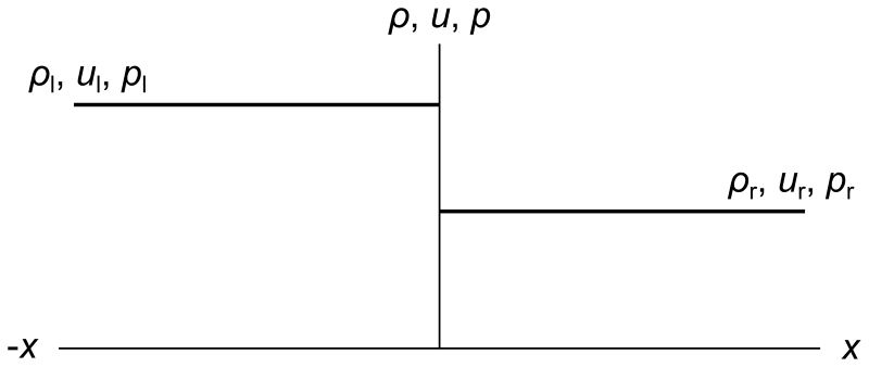
Look familiar? Yes, that is just the initial condition for our 1D shock tube problem. Thus, Riemann solvers, which solve the Riemann problem, are incredibly useful for solving hyperbolic equations to treat discontinuities that may arise. The Riemann solver provides us with a better resolution of the shockwave and thus protects us, to some extent, from numerical diffusion near sharp gradients.
So you may then be wondering, having just talked about the artificial compressibility method, why on earth do you want to have a hyperbolic system for incompressible methods? Aren't we just complicating things by now allowing shock waves (discontinuities) to exist in our flow? The answer is yes and no.
Yes, because we now have to deal with potential discontinuities, thus requiring shock-capturing schemes we have developed for compressible flows. However, these are all fairly standard knowledge these days in the field of CFD and are easy to access and implement. On the other hand, hyperbolic equations do not make our life more complicated because we already have discontinuities in incompressible flows, regardless of the type of the PDE! Take the following figure, for example:
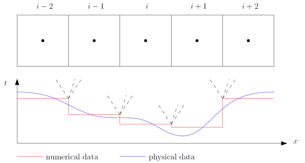
Here, I show five cells that store some physical properties (velocity, pressure, temperature, etc.) at their centroid values. If we are using a finite volume discretisation, then we assume that the data within a cell is constant, and we take the centroid value everywhere in the cell. This also means that when we approach a face that is shared between two cells, we naturally create a discontinuity. This is shown by the graph below the cells, where the real, physical solution is smooth (shown in blue), but the approximated solution (red) contains discontinuities.
Godunov, another great name to remember in the field of CFD, saw this as an opportunity and postulated that we should employ a Riemann solver for each face (opposed to using a Riemann solver just for a single discontinuity, for example, to compute the solution of the shock tube problem). This is what we know as the Godunov method nowadays.
Thus, regardless of the flow (incompressible or compressible), we always have to deal with discontinuities. For compressible flows, these may be stronger, as our discontinuities arising from the numerical data is enhanced by the discontinuities of the physical data (e.g. shock waves), but both flows would benefit from Riemann solvers and thus the artificial compressibility method is a viable method to solve incompressible flows!
Parabolic flows
Ok, we have gotten a flavour for hyperbolic flows. Let's turn our attention now to parabolic flows. These are classified as having real but not distinct characteristics, i.e. there is only a single characteristic. How does it manifest itself in flows? Again, we can observe parabolic behaviour in real flow scenarios. Take the flow in a boundary layer, for example. This is schematically shown below:
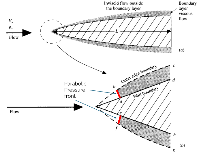
If we consider the flow within the boundary layer, we can see the flow passing through a single front which I have labelled here the parabolic pressure front (which is a great name for an alternative avant-garde vegan movement! Fell free to become the self-proclaimed leader). Whenever we have a single pressure front, which is driving the flow, we have a parabolised behaviour.
Sometimes the flow itself is hyperbolic; just because we only see a single characteristic doesn't mean that we necessarily have a parabolic system. It may simply mean that there is only one characteristic we can easily see from the visualisation (similar to the hyperbolic flow above, where we saw clear shock waves at the leading and trailing edge but not elsewhere in the flow, although real and distinct characteristics existing at each point in the flow).
But what happens if you have a parabolic system and then simulate it? Well, yours truly spent a good portion of his PhD developing, testing, and implementing parabolic versions of the Navier-Stokes equations for incompressible flows. Why? As it turns out, they allow for fast solutions in unsteady flows, which is always a positive side-effect, but it also means that I can simulate some parabolic flows for you and you can observe the way the pressure is behaving:
So, what can we see? Some pressure waves travel back and forth in the channel, representing a uniform front, i.e. the pressure waves appear to be straight lines, apart from slight deviation near the step. To be fair, hyperbolic equations would produce a very similar flow pattern here, but this example lends itself well to exploring parabolic equations, as the flow is restricted naturally between two walls at the top and bottom (similar to the boundary layer equation discussed above).
Whenever we have a bounding geometry or flow, we can see these pressure waves travelling through our domain. What I did not disclose here are the equations that govern this flow, and they are not of importance here, really, except that the continuity equation was used with a time-derivative of some description. The time derivative, again, is what turns this equation from a purely elliptic to a parabolic system.
Hyperbolic and parabolic equations are actually quite similar and related in the way that we solve them. While we can't use Riemann solvers for parabolic equations, both hyperbolic and parabolic equations have one thing in common: the time derivative. Without the unsteady behaviour, the system would be elliptic. Thus, whenever we are dealing with either hyperbolic or parabolic equations, we are dealing with a time-marching solution.
If we are interested in a steady-state solution, we simply run the simulation until all transient behaviour has washed out and we are left with a flow that does not change in time, or where there is still a transient behaviour but we can average the solution to obtain a more steady-state-like behaviour.
So why is dealing with a time-marching solution efficient? In a nutshell, non-linearity. The non-linear behaviour of the Navier-Stokes equations requires us to carefully consider our solution strategy; otherwise, we will run into divergence problems. As a result, we typically under-relax equations (meaning we only apply a fraction of the computed solution) to dampen any oscillatory motion and, thus, divergence.
The time step size is directly proportional to the under-relaxation factor, which is shown in the following schematic:
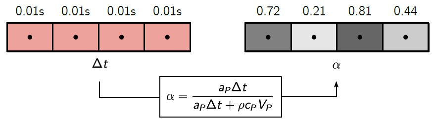
Here, [katex]\alpha[/katex] is the under-relaxation factor, and [katex]a_P[/katex], as well as [katex]c_P[/katex] are coefficients that come out from the discretisation. We see that if we have a constant time-step for each cell (shown on the left), we get different under-relaxation factors for each cell (on the right).
In other words, if I know that my solution ought to be steady-state, and I just want to march as quickly to that solution as possible, then why not set a time step in each cell that maximises the convergence, i.e. set the time-step to a value that sets the under-relaxation factor in each cell to the same (max) value? This is what is known as local time stepping, where each cell gets its own timestep size. It has proven to work well, except in the case of OpenFOAM, where it is implemented but is not working, as with so many other things in OpenFOAM.
So, whenever we have a parabolic or hyperbolic flow, we want to make use of shock-capturing schemes (hyperbolic only) to enhance precision (and usually, as a result, accuracy). We also want to employ time-marching solutions so that we get fast convergence to a steady-state solution.
If our system is steady-state, we may still add an artificial time derivative purely for better convergence behaviour. This is known as pseudo-time stepping, where the time derivative may not have any physical meaning but is only used to speed up the convergence. If you are using ANSYS Fluent, you will have access to a bunch of different pseudo time methods, all working excellently to reduce oscillations and thus speed up the convergence rate.
Why does it speed up convergence? Well, in order to understand that, we first need to talk about elliptic equations.
Elliptic flows
We looked at the backward facing step problem above and looked at the development of the pressure. We said that parabolic equations have real characteristics which are all the same. Elliptic equations, on the other hand, have only imaginary characteristics. What does that mean? Well, let's look at the pressure behaviour for the same case:
As you can see, you can't see anything (in terms of characteristics!). This means that if there aren't any real characteristics (all eigenvalues are imaginary), then there is no preferred mechanism for the pressure to spread. We won't get any pressure fronts, and instead, the pressure is just propagating throughout the domain however fast it wishes. In fact, this is one of the character traits of elliptic equations: A disturbance created in one point of the domain will influence the rest of the domain instantaneously.
Let's look once again at the flow around an airfoil. We are now looking at an incompressible flow. We discussed above that an incompressible flow, especially a steady-state flow, will have a mixed elliptic-hyperbolic behaviour. So, how can we see this elliptic behaviour? Consider point A in the figure below:
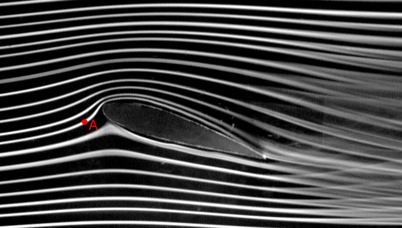
How does the flow at point A know that it has to curve upwards so to flow over the airfoil? At point A, the flow hasn't seen (or felt) the presence of the airfoil, yet it deflects upwards. The answer is that the flow is elliptic. Once the first particle hits the airfoil, it will propagate that information (through pressure waves) back upstream, so the flow at point A will be influenced by the disturbance created downstream of point A.
If this sounds abstract, think of it from a molecular point of view. Once an atom, or a particle, hits the surface, it is being deflected. Some will go up, some will go down, but some will be pushed back upstream. These particles will then collide with other particles upstream, say, at location A, which will then be deflected as a result. Thus, disturbances are felt instantaneously throughout the domain.
How do we solve elliptic equations then? Well, you would think that this instantaneous spreading of information (pressure) is a good thing, allowing for fast convergence of our pressure. You would be right, if the pressure and velocity are decoupled, but, the momentum equation tells us that both are closely coupled. Even if the pressure can spread quickly, it will always be held back by the velocity through the momentum equation.
However, if you have a purely elliptic equation, say the steady-state heat diffusion equation, then you observe the magic of true elliptic equations. Changes can propagate as fast as you allow them through the domain, and the faster they can propagate, the faster your convergence will be. Multigrids have been specifically developed to take advantage of this fact, and if you have to solve purely elliptic equations, you want, nay, must use a multigrid approach if you want to get insane convergence rates.
We stopped the parabolic section above, stating that it may be advisable to introduce some form of pseudo-time stepping to accelerate convergence. This may seem counterintuitive; if we introduce a time derivative, or time-dependence in general, we restrict the amount of information (pressure waves) that can travel in each time step. This is directly linked to the timestep. A small time step will propagate information slower than a larger time step, and thus converge slower as well.
So why would you add a time derivative to an elliptic system, which is supposed to have insanely fast convergence properties? Well, in the case of the Navier-Stokes equations, it comes back to pressure-velocity coupling and the non-linear term. Changing too drastically can introduce divergence. Or you may get stable but highly oscillatory results.
If you are playing golf, you have different golf clubs for different distances. You have your drivers to get your golf ball across large distances and then your putters for precision near the hole. Imagine using a long-range driver near the hole; you would constantly overshoot the hole. You may have a similar behaviour with elliptic equations; they just constantly overshoot the steady-state solution.
Thus, introducing a time derivate limits the speed of information propagation (which essentially introduces under-relaxation), which in turn stabilises the non-linear term, which in turn results in better convergence.
A speed limit on the road will force you to take longer to get to your destination, but it also correlates well with a lower risk of being in an accident. Risk and reward. Your choice, how much speed do you want in your CFD results? More speed (larger time step), faster convergence, more oscillation (potentially). As always, there is a balance, and you'll have to find it.
Summary
Right, we have covered a lot of ground here, and I hope you have gotten a bit of a better idea of why the classification into hyperbolic, parabolic, and elliptic equations is not just useful but essential to select suitable numerical schemes.
We looked at the classical textbook definition of how to classify second-order partial differential equations (PDEs), and then introduced a more generalised approach for systems of first-order PDEs, as well as mixed-order PDEs.
We classified the Navier-Stokes equations as being fully hyperbolic for compressible flows and mixed elliptic-hyperbolic for incompressible flows. Then, using the concepts of characteristics, we were able to link the classification procedure to real physical properties in the flow that we can visually see from CFD results.
Finally, we looked at hyperbolic, parabolic, and elliptic equations and what their solutions looked like. I hope that this will help you to develop an intuition for how these equations behave and what the physical importance of these equation types is. Before we close, I want to return one last time to the classical textbook definition we have seen a few times above. By now, you should understand it in its entirety, otherwise I have done a poor job in explaining it! Here it is:
Hyperbolic PDEs have real and distinct characteristics, while parabolic PDEs have real characteristics, which will have the same value. Elliptic PDEs, on the other hand, have only imaginary characteristics.
Clear now? Great! I'll see you in the next article.
Acknowledgements
Special thanks to Alexander Schukmann for helping me to improve this article! Check out how you can contribute, too.

Tom-Robin Teschner is a senior lecturer in computational fluid dynamics and course director for the MSc in computational fluid dynamics and the MSc in aerospace computational engineering at Cranfield University.