How to implement boundary conditions in CFD

In this series thus far, we have looked at the governing equations of CFD, how to discretise them and what their character is. We have looked at different numerical schemes and how they influence various properties, such as accuracy. Eventually, we need to talk about boundary conditions, as every simulation will have to truncate the simulation domain somewhere.

Thus, in this article, we take a deep dive into the (fascinating?!) world of boundary conditions, and I promise you, you might think they are easy and straightforward (I’ve been there), but they are not. The devil is in the detail, and by the end of this article, you will have an appreciation for what common issues, solved and unsolved, exist when we have to deal with boundary conditions.

In the process, we will see that there really are only three different types of boundary conditions, and if you understand them, you can model any kind of boundary. In most cases, we don’t even need the third, so just knowing two, really, is all you need. With these two (or three) fundamental types of boundary conditions, we can derive boundary conditions like walls, symmetry planes, inlets, outlets, and so on, which are just different combinations of these two fundamental types of boundary conditions for the flow variables we are solving for.

I can’t make boundary conditions look sexy, but I can tell you about all of the dead bodies it has been hiding and its troubled past (and future), if that is something you are interested in, get the popcorn, we have a journey in front of us!

In this series

• Part 1: How to Derive the Navier-Stokes Equations: From start to end
• Part 2: What are Hyperbolic, parabolic, and elliptic equations in CFD?
• Part 3: How to discretise the Navier-Stokes equations
• Part 4: Explicit vs. Implicit time integration and the CFL condition
• Part 5: Space and time integration schemes for CFD applications
• Part 6: How to implement boundary conditions in CFD
• Part 7: How to solve incompressible and compressible flows in CFD

In this article

Introduction

When you performed your first CFD simulations, you probably simulated some kind of laminar or even turbulent flow using a commercial or open-source solver. You selected some boundary conditions, perhaps a combination of inlets and outlets, and sprinkled in some solid walls here and there. You solved this simulation, got results, and presumably, you were very happy with the results. If this describes you, then you would be forgiven for thinking that imposing boundary conditions is easy.

Well, a lot happens behind the scenes, which is abstracted away from you. Unless you deal with OpenFOAM (where the developers really want you to think long and hard about your boundary conditions, and, by extension, about your life choices (I could have used Fluent/StarCCM+ instead …)), the end result you see is a combination of violated physics and some undisclosed black magic. Let’s face it: we probably all go to hell for the way we treat boundaries. We don’t want to admit it, but we know it to be true in our hearts. Or is it just me?

When I applied for my first PhD position on Large Eddy Simulations (LES) and Direct Numerical Simulations (DNS), I was invited for an interview, and I got into a heated argument with one of the post-docs. He was working in the wind tunnel (and, as you are probably aware, there is a healthy portion of distrust and hatred between computational and experimental fluid dynamicists!). So naturally, I didn’t take his opinions on CFD too seriously. He insisted that boundary conditions are one of the hardest things to get right, whereas I was of the opinion that they are easy.

I got offered the PhD position (to everyone’s surprise, including mine), and later found myself trying to implement boundary conditions into my Cartesian grid-based solver in 2D for steady, laminar flows (we experts call this piss-easy, yes, this is scientific terminology …). To my surprise, I was struggling, and while I was trying to resolve my boundary condition issues after spending months going through the literature and looking for answers, I remembered the discussion I had with the post-doc. Could he have been right?

Later, I was working on a project using Large-Eddy Simulations. I also supervised a PhD student at the time working on high-resolution schemes on unstructured grids for external aeronautical applications. We both were suffering from the boundary conditions. My inlet boundary conditions could only be described as borderline illegal, while my PhD student did confess to me, after 9 months of troubleshooting, that he just copied and pasted boundary conditions from a different case. After I made some modifications, his case worked, but now he is going to hell, too (I guess).

Boundary conditions are hard. If you believe they aren’t, then you either have never implemented them yourself or have done any simulations where the adverse effects of boundary conditions become an issue. If you want to challenge yourself, go and set up a channel flow with Large Eddy Simulations. But no cheating; periodic boundary conditions aren’t allowed. You will realise that there are as many different boundary conditions you can impose at the inlet as there are probably RANS turbulence models available, and some are better than others but not necessarily more correct.

In 1991, Sani and Gresho (who would also later publish their book on finite elements in CFD applications) held a mini-symposium on open questions and challenges for open boundary conditions during the seventh international conference on numerical methods for laminar and turbulent flow. Three years later, they would publish a bleak review of the outcome of this mini symposium.

The test cases they discussed were classical test cases such as the steady-state flow over a backward-facing step (with and without heating), the unsteady flow past a circular cylinder, and the steady-state flow through a channel. But these cases came with a twist; test cases needed to be simulated with boundary conditions imposed in two locations.

The first location was far downstream, i.e. far enough away so that they would not influence the simulation. However, the second location was in a region where the flow was still developing. For example, for the circular cylinder case, the boundaries were placed as close as four diameters away from the cylinder. The von Karman vortex shedding is still in development in this region.

The participants presented results for different outlet boundary conditions, and in their 1994 review, Sani and Gresho summarised the mini-symposium and its outcome as:

It has been an exercise in frustration and we are not thrilled with the results obtained

Sani and Gresho, 1994

You would think that 30+ years later, we would have solved all of these issues. We haven’t. Sure, we have made some advances in specific areas, such as inlet boundary conditions for scale-resolving turbulent flows, but we are still struggling with very fundamental problems. If you have ever worked with Fluent, for example, then you might have encountered reverse flow on the outlet. Once that happens, your convergence is affected, so the developers at Fluent have implemented a fix.

What’s that fix? Well, if you encounter reverse flow on a specific cell at the outlet, Fluent will temporarily turn that cell into a wall, preventing flow from entering. Genius, right? Now, you tell me if this is a true reflection of the physics that is going on or a quick and dirty fix we have come to accept because we haven’t made any advances in the past 30 years.

The fundamental problem with boundary conditions

Before we now go into deep philosophical discussions on boundary conditions, let’s address the issue at hand. Why are they so difficult? Why can’t we make advances in this field?

The short and simple answer is: because boundary conditions don’t exist in real life, at least not all!

To see that this is true, let us look first at boundary conditions that do exist. These are solid boundaries, i.e. walls. In a computational sense, nothing can penetrate a solid boundary, i.e. fluid can’t go through a wall (unless we impose some form of porosity, which I am ignoring in this example). In real life, we do have physical wall-type boundaries as well. The cup I had my tea in this morning (Madam Grey, two sugars, and a flood of milk, apparently called a builder’s brew …) effectively held the fluid in one place. There was no dripping or loss of fluid.

If you want to simulate the flow around an airfoil and also decide to run some wind tunnel experiments (of course, without telling your friends, you don’t want to be seen hanging out with those experimental people!), then you can go into the test section and physically touch the wing that is installed in the wind tunnel.

Solid boundaries can be found in real life and, thus, are easy to model. But what about open boundaries like inlets and outlets? Think about it for a second. Can you come up with an example of an inlet or an outlet in real life? You can? Well, think again. There are no such things as inlets and outlets or, in general, open boundaries in real life. Every system is connected to another system in some way.

If you simulate the flow through a pipe, whatever you impose at the inlet has to come from somewhere, a part of the system that you have conveniently ignored to model in your simulation. Or go back to the example of the airfoil simulation. In the wind tunnel, whatever leaves the test section (i.e. what we would call an outlet in a CFD simulation) is recycled, straightened, and pressurised before it is returned through the wind tunnel to the test section (i.e. what we would call an inlet in a CFD simulation).

There are no open boundaries in real life, and if you want to have a physically correct system, then you are only allowed to use solid walls as your boundary condition. Take the wind tunnel, for example. Instead of imposing a fixed inlet velocity, you could also model the entire wind tunnel, including the spinning rotor, which would drive the flow. This geometry would consist of only walls and thus be a valid physical representation. But as soon as you chop off parts of the system and model the effect of the rotor through an inlet, you have changed the original system.

For a steady state RANS simulation, this might be OK, but you will still have to impose boundary conditions for your RANS model. If you are solving this flow with the k-\omega SST model, for example, you will need to impose boundary conditions at the inlet for the turbulent kinetic energy k and the specific dissipation rate \omega. Are you confident that you can impose correct values for these quantities? And is a uniform distribution of k and \omega across the inlet plane a good approximation or would you expect these quantities to be non-uniformly distributed?

Turbulent kinetic energy is created in boundary layers, so close to the walls, and where you have turbulent kinetic energy, you have dissipation. Thus, you probably have much more happening at the edges of your inlet, where your inlet intersects with a solid wall. OK, so how tall is the turbulent boundary layer at your inlet? After all, you have chopped off part of the system; if there was no inlet, then we would have some boundary layer at the wall. You need to know the size of the turbulent boundary layer in order to impose realistic values for k and \omega here.

Thankfully, the values of k and \omega are not very sensitive to changes, so you will still get fairly good results in most cases, even if you can’t accurately describe these values at the inlet. This is one positive attribute of RANS models. But once you want to resolve more turbulence, rather than modelling it, i.e. we are talking about scale-resolving turbulence such as Detached-eddy Simulations (DES), Scale-adaptative Simulations (SAS), Large-eddy Simulations (LES), or god forbid, even Direct Numerical Simulations (DNS), then the above discussed issues become a real problem!

Because we are now resolving turbulence, we also need to resolve the boundary layer at our inlet. If we don’t, well, then we are solving a different type of flow. So how do we get around this issue? Well, there are several solutions in the literature, all of which are an approximation, but none of them are correct.

The simplest approach is to give up before we even start, waive a white flag and pretend that there is no turbulence at the inlet. In this case, we set all turbulence to zero and only impose freestream conditions for velocity, pressure, and potentially temperature. This is the simplest approach and, in some cases, a good approximation. Wind tunnels are able to suck away unwanted boundary layers, so as long as we place our inlet at exactly the position where the boundary layer is sucked away and we develop a new boundary layer, we should be golden, right?

Perhaps, and thinking only about the velocity, this is likely a good approximation. But what about the pressure? We looked at elliptic flows in an earlier article within this series, and the pressure is, for the most part, governed by an elliptic behaviour. What that means is that a change in pressure in one point of the flow will instantly propagate throughout the domain. This is why your flow starts turning around an obstacle before it has even reached it. Look at the streamlines around an airfoil, as shown in the above-linked article, to see what I mean.

What this means for our simulation is that by placing an inlet somewhere, we restrict the propagation of pressure (waves) only in a direction away from the inlet. The pressure isn’t allowed to go beyond the inlet, influence the velocity upstream of the inlet itself, and, as a result, change the velocity profile that would otherwise develop at the inlet. This may seem like a small thing, but always remember that the Navier-Stokes equations are non-linear. A small change can have large consequences. After all, turbulence is created by microscopic surface roughness (natural transition).

You can show (and I have) that removing an upstream portion of the flow and replacing this with an inlet with a defined velocity profile that was measured in an experiment will give you different results compared to just simulating the upstream portion of the domain. It is the pressure that plays a critical role here, and concentrating only on the velocity will result in inaccuracies.

Of course, if you are dealing with supersonic flows, your pressure is hyperbolic, meaning that it has a preferred direction of travel, unlike elliptic flows, where it is travelling in all directions, and so imposing an inlet here is easier. While you have gained simplicity at the inlet, you have shifted the problem to the numerical schemes, which now have to deal with strong non-linearities. We saw in the last article how to tackle those. Alas, not every flow is supersonic, so we are stuck with elliptic pressure-induced boundary issues.

Hopefully, this will set the scene for you. Boundary conditions aren’t easy, but they are a necessary evil that we have to deal with in any simulation. In this article, I want to look at how boundary conditions are commonly imposed, and we will see that there are really just three fundamental types of boundary conditions, of which the third type is just a combination of the first two. So, if you understand these two fundamental boundary conditions, you know all there is about boundary conditions. The art is in finding a combination that works for your case that doesn’t violate the laws of physics (good luck to you, my friend!)

Three fundamental boundary conditions to rule them all

In this section, we will review the three fundamental types of boundary conditions that we can use in simulations. The first two types are the ones you will use in every simulation. When you use a CFD solver and you select a type for your boundary, for example, a wall, or an inlet, your solver will use that information and translate that back to the two fundamental types for all of the quantities that you are solving for, e.g. velocity, pressure, temperature, and any turbulent quantities.

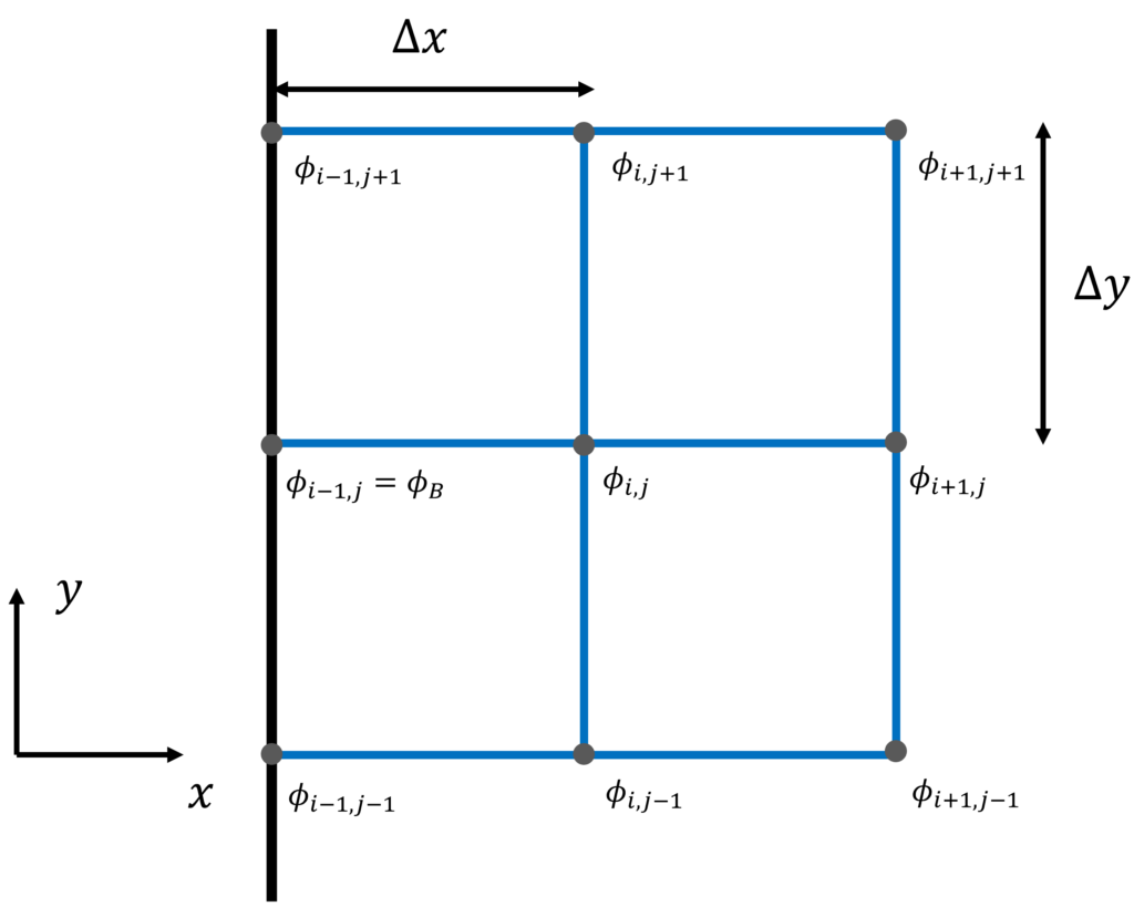
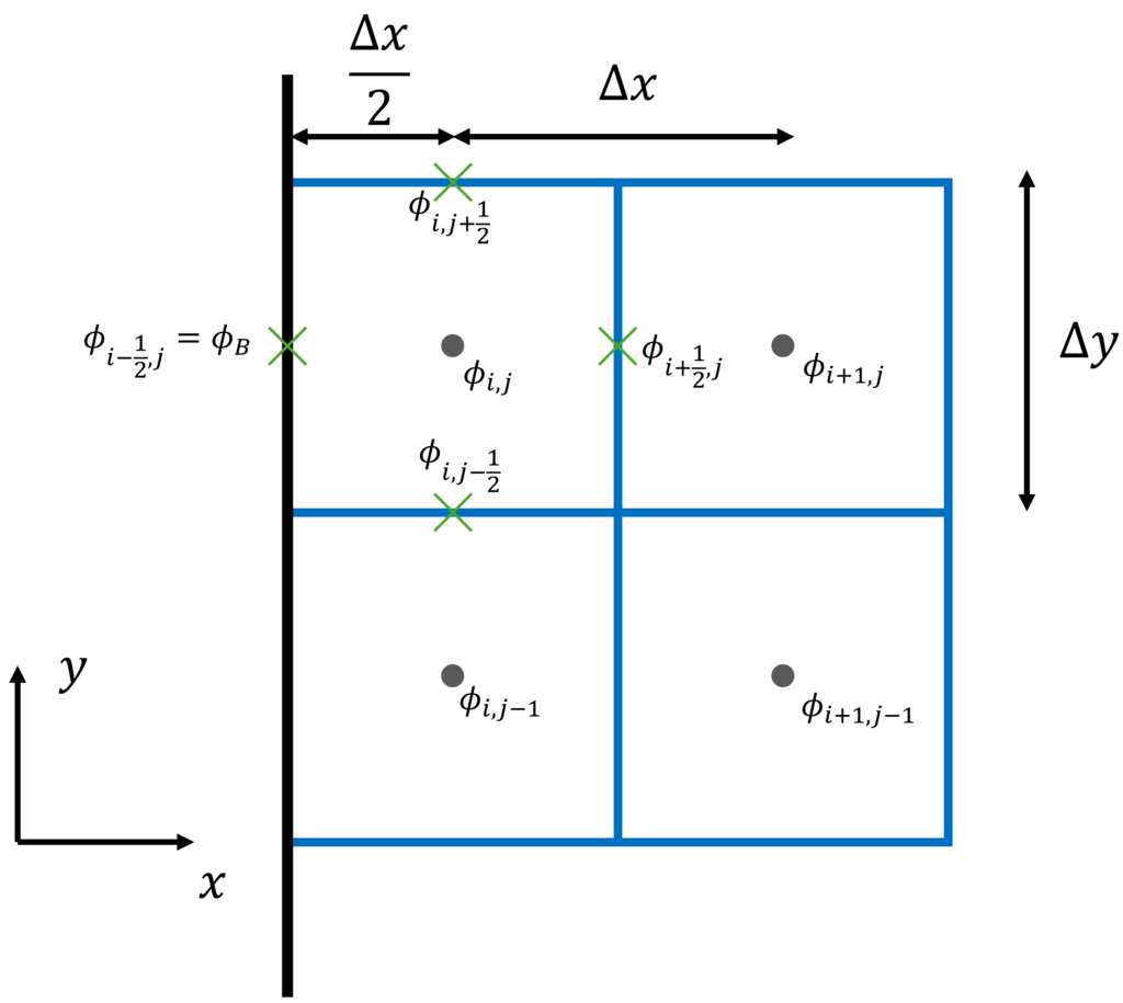
To make our lives easier, let’s introduce some notation that we will use to derive the three fundamental types of boundary conditions. The two figures below show the cell arrangement commonly found in the finite difference method (left side), where the variables are stored at the cell’s vertices, and the cell arrangement commonly found in the finite volume method (right side), where the variables are stored at the cell’s centroid.

Vertex-based boundary conditions (finite difference method)

Centroid-based boundary conditions (finite volume method)

Dirichlet-type boundary conditions

Dirichlet-type boundary conditions are those where we impose a value directly. For example, we can impose a velocity, say 10 m/s at an inlet, and then all velocity at the inlet will have this value. This means that we need to know the value we want to impose and that this value will be typically uniformly distributed across the boundary, though we can also implement a non-uniform distribution if we know how this distribution will look like. For example, we may know the velocity profile from experiments.

Let’s see how this can be implemented for the two types of grids that we saw above. On the left, we have the typical vertex-based arrangement that we normally use for finite difference methods. If we concentrate on \phi_{i-1,j}, which simply refer to as \phi_B, i.e. the value of \phi at the boudnary, then we see that since this node is already located on the boundary, we can simply write

\phi_{i,j-1}=\phi_B =\phi_{Dirichlet}

Here, \phi_{Dirichlet} is the value we want to impose on the boundary, e.g. 10 m/s on an inlet, 0 m/s at a non-moving wall, etc. This is rather straightforward. But what about the case on the right side of the figure?

Well, the right side of the figure shows the typical cell arrangement for a finite volume discretisation. We can see that the node on the boundary is not the cell centroid, i.e. the location where we store our flow variables like velocity, pressure, temperature, etc., but rather \phi_{i-1/2,j}=\phi_B. Again, we just pick one point on the boundary, but the discussion would be the same for any of the other boundary points.

Let’s review the finite volume discretisation again. In my article on how to discretise the Navier-Stokes equations, we looked at how to derive first-order and second-order derivatives. For the first-order spatial derivatives (i.e. in space), we obtained this approximation:

a\int_V\frac{\partial \phi}{\partial x}\mathrm{d}V=a\int_An\cdot\phi\,\mathrm{d}A\approx a\sum_{i=1}^{n_{faces}}n_f\cdot \phi_i A_i

Here, a is some coefficient, for example, the linearised velocity in the non-linear convective term. We go from a volume integral to a surface integral using the Gauss or divergence theorem, which requires us to integrate over all cell faces. In the finite volume method, we approximate that integration by a summation, where we now have to the face normal vector n_f, as well as the face area A_i.

What about \phi_i? Well, these are the values of \phi at the cell’s faces. This is indicated in the figure above on the right by the green crosses on the faces. So, using the figure’s notation, we could write this summation explicitly as:

a\sum_{i=1}^{n_{faces}}n_f\cdot \phi_i A_i=a\left[(\phi_{i+1/2,j}\Delta y) + (\phi_{i,j+1/2}\Delta x) - (\phi_{i,j-1/2}\Delta x) - (\phi_{i-1/2,j}\Delta y)\right]

The plus and minus signs appear as a result of the orientation of the normal vector. The convention is that it is pointing outwards, so on the right and top face, the normal vector is pointing along the x and y direction, respectively, so we multiply the flux \phi_i A_i with +1 in the x and y direction. For the left and bottom face, on the other hand, the normal vector points against the x and y direction, so we multiply the fluxes by -1, hence the negative sign.

If we look at the discretised form above, then we see that our Dirichlet value has sneaked into the discretised equation, i.e. the last term \phi_{i-1/1,j} is located on the boundary, and thus we could also write this as \phi_{i-1/2,j}=\phi_B=\phi_{Dirichlet}. Then, our discretised form becomes:

a\sum_{i=1}^{n_{faces}}n_f\cdot \phi_i A_i=a\left[(\phi_{i+1/2,j}\Delta y) + (\phi_{i,j+1/2}\Delta x) - (\phi_{i,j-1/2}\Delta x) - (\phi_{Dirichlet}\Delta y)\right]

Now we can solve this equation again, by finding values for the remaining values of \phi_{i+1/2, j}, \phi_{i,j+1/2}, and \phi_{i,j-1/2} through a suitable numerical scheme. We have looked at suitable numerical schemes for the finite volume method in the previous article.

But we also have to deal with second-order derivatives, which are slightly different. Again, I have derived their step-by-step derivation in the article on how to discretise the Navier-Stokes equation, so we will just look at the final form here, which is of interest. We saw that we can write the finite volume approximation for the second-order derivative as:

b\int_V \frac{\partial^2 \phi}{\partial x^2}\mathrm{d}V=b\int_V \frac{\partial}{\partial x}\frac{\partial \phi}{\partial x}\mathrm{d}V\approx b\sum_{i=1}^{n_{faces}}n_f\cdot \frac{\partial \phi_i}{\partial x} A_i

Here, b is some coefficient, but since we only have the diffusion term in the Navier-Stokes equation that uses a second-order derivative, this means that b will always be the dynamic or kinematic viscosity (depending on whether it is divided by the density or not).

So now we have the derivative to deal with in our summation. Let’s look at the face on the right, i.e. at location i+1/2,j. Looking at the above figure, we can see that a simple approximation for the derivative at this face could be written as

\frac{\partial\phi}{\partial x}\biggr\rvert_{i+1/2,j}\approx\frac{\phi_{i+1,j}-\phi_{i,j}}{\Delta x}

But what about the left face? Here we do not have a value beyond the location i-1/2,j, so we can evaluate the gradient the same way. In this case, we simply form the gradient between locations i-1/2,j and i,j, which results in

\frac{\partial\phi}{\partial x}\biggr\rvert_{i-1/2,j}\approx\frac{\phi_{i,j}-\phi_{i-1/2,j}}{\Delta x/2}=2\frac{\phi_{i,j}-\phi_{Dirichlet}}{\Delta x}

Now we see the appearance of \phi_{i-1/2,j}=\phi_B=\phi_{Dirichlet} again, and so we can impose our Dirichlet-type boundary condition for second-order derivatives again. We would find suitable approximations for the remaining terms, i.e. \phi_{i,j+1/2} and \phi_{i,j-1/2}, and then we can continue with our finite volume approximation.

The remaining steps to approximate both the first-order and second-order derivatives, as well as how to bring them into a form that can be easily solved, are discussed in the previously mentioned article on how to discretise the Navier-Stokes equations.

Neumann-type boundary conditions

Neumann-type boundary conditions are really just Dirichlet-type boundary conditions in disguise. Instead of setting the absolute value of a quantity \phi (e.g. velocity, pressure, temperature, etc.) at the boundary, we set the value of its derivative, i.e. \partial\phi/\partial n, where n is the normal vector on the boundary.

We use this boundary condition when we do not know the values at the boundary and we want them to be calculated as part of the solution. Let’s take a simple example, a simple flow through a channel, with an inlet, an outlet, and a wall at the top, bottom, front, and back.

For simplicity, let’s say we want to impose a velocity at the inlet that is constant across the inlet boundary. What, then, is the velocity at the outlet? We don’t know. We would expect it to follow some form of parabolic or power-law velocity profile depending on whether it is a laminar or turbulent flow, but if our domain is very short, it might not even fully develop. We don’t know how the velocity will be distributed at the outlet, so we pick a Neumann-type boundary condition for the velocity at the outlet.

Now, let’s look at the pressure. If we assume that the outlet is connected to some opening where we have atmospheric conditions, then it would make sense to prescribe the atmospheric or ambient pressure at the outlet. This can be a constant value for the pressure across the boundary, so we would impose a Dirichlet-type boundary condition for the pressure at the outlet.

What about the inlet? There will be a pressure drop within the channel, but we don’t know what its magnitude is. If we want the pressure drop to develop as part of the solution, then we need to allow the pressure to freely develop at the inlet boundary, as the difference of the pressure at the inlet and outlet will determine the pressure gradient (if we divide the difference by the channel length). Thus, we need a Neumann-type boundary condition for the pressure at the inlet.

Finally, what about the walls? We know that we have a no-slip condition, so the velocity should have the same value as the translational motion of the wall. Typically, walls are stationary in simulations, so there is no movement of the walls, and that means our velocity in each direction has to be zero. Since we know the value, we have to impose a Dirichlet-type boundary condition for the velocity at solid walls.

Now, think about the pressure distribution around an airfoil. It changes from the leading edge to the trailing edge. The only thing we can say with confidence is that the pressure coefficient is one at the stagnation points. However, we don’t know the distribution between the leading and trailing edges. The same is true for our channel example, we don’t know the pressure here, so we need to let it develop as part of our solution. This means that the pressure needs to be treated as a Neumann-type boundary condition at solid walls.

So, let’s see how we can impose Neumann-type boundary conditions. In general, we can write them as follows:

\frac{\partial \phi}{\partial n}=\phi_{Neumann}

Here, n is the direction of the normal vector on the boundary. In the figures we looked at above, we have n=x, i.e. it is aligned with the x-direction. Using the notation of n allows us to write the boundary condition in a generic notation or even account for curvature on the boundary.

\phi_{Neumann} is the value the derivative should be equal to. A common choice is to set \phi_{Neumann}=0. But there are cases where we want to impose a non-zero value for \phi_{Neumann}, for example, when we are dealing with heat transfer applications (where \phi=T) and we want to impose some heating, which would be realised with a non-zero gradient of the temperature gradient at the wall (i.e. we set a heat flux).

So, let’s start to see how we can impose Neumann-type boundary conditions on the domain sketched out in the figures we looked at previously. For the figure on the left, i.e. using the finite difference method, we have the following discretisation:

\frac{\partial \phi}{\partial n}=\frac{\partial \phi}{\partial x}=\frac{\phi_{i,j}-\phi_{i-1,j}}{\Delta x}=\frac{\phi_{i,j}-\phi_B}{\Delta x}=\phi_{Neumann}

Now, all that we have to do is solve this equation for \phi_B, which will be the value at the boundary that we will impose. This will lead to:

\phi_B=\phi_{i,j}-\Delta x\cdot\phi_{Neumann}

The boundary position is important and changes this calculation. For example, if we assume for a second that the boundary would be located at i+1,j in the figure, i.e. the solid, vertical black line would be attached to the blue cells on the right, then our boundary condition would be evaluated as:

\frac{\partial \phi}{\partial n}=\frac{\partial \phi}{\partial x}=\frac{\phi_{i+1,j}-\phi_{i,j}}{\Delta x}=\frac{\phi_{B}-\phi_{i,j}}{\Delta x}=\phi_{Neumann}

In this case, when we solve for \phi_B, we obtain:

\phi_B=\phi_{i,j}+\Delta x\cdot\phi_{Neumann}

Now, if we have the special case of \phi_{Neumann}=0 (in the channel flow example we discussed above, all Neumann-type boundaries had a zero gradient condition), both expressions simplify to

\phi_B=\phi_{i,j}

That is, we simply copy the value of \phi that is next to our boundary node in the n direction. Now you can see why I said that Neumann-type boundary conditions are Dirichlet-type boundary conditions in disguise. We still impose a value for them, but we do so with values from the internal domain. This is also why the values can change (like the pressure distribution around an airfoil), which is based on values obtained from the internal fluid domain.

And what about the finite volume discretisation? Switching our attention to the figure on the right, which we saw in the beginning of this section, we have a very similar process. We can write the Neumann-type boundary condition as

\frac{\partial \phi}{\partial n}=\frac{\partial \phi}{\partial x}=\frac{\phi_{i,j}-\phi_{i-1/2,j}}{\Delta x/2}=2\frac{\phi_{i,j}-\phi_B}{\Delta x}=\phi_{Neumann}

We can solve this equation now for \phi_B, which results in

\phi_B=\phi_{i,j}-\frac{\Delta x}{2}\phi_{Neumann}

If the boundary would be located again at i+1,j, i.e. on the east side of the simplified domain given in the figure above, then we would obtain

\frac{\partial \phi}{\partial n}=\frac{\partial \phi}{\partial x}=\frac{\phi_{i+3/2,j}-\phi_{i+1,j}}{\Delta x/2}=2\frac{\phi_{B}-\phi_{i+1,j}}{\Delta x}=\phi_{Neumann}

Here, the location i+3/2,j is the face between i+1,j and i+2,j, i.e. i+3/2,j=i+1.5,j. Then can then be solved for \phi_B again to result in

\phi_B=\phi_{i+1,j}+\frac{\Delta x}{2}\phi_{Neumann}

If we have \phi_{Neumann}=0, then we can simplify our expression again, and we have

\phi_B=\phi_{i,j}

For the arrangement given in the figure above on the right (i.e. the boundary is located on the west face of the domain). Since we know the value on the Boundary now, we can continue exactly in the same way as we did for the Dirichlet-type boundary condition. And this is what I would advocate you should do if you want to write your own solver.

Some CFD textbooks will introduce a simplification for second-order derivatives. We saw in the discussion on the Dirichlet-type boundary conditions that we had the following expression for second-order derivatives:

b\int_V \frac{\partial^2 \phi}{\partial x^2}\mathrm{d}V=b\int_V \frac{\partial}{\partial x}\frac{\partial \phi}{\partial x}\mathrm{d}V\approx b\sum_{i=1}^{n_{faces}}n_f\cdot \frac{\partial \phi_i}{\partial x} A_i

Since we now have to deal with derivatives directly, as seen in the last term, when we are summing over all faces, we could simply set the gradient at the boundary to the value of \phi_{Neumann}.

I don’t like this approach because this is not how you want to implement that in code. Based on the discussion we had up to this point, we saw that once we have found a way to implement Dirichlet-type boundary conditions, we can reuse (or even better, modify) this implementation to also allow for Neumann-type boundary conditions. This results in cleaner code, which is easier to maintain and modify.

Robin-type boundary conditions

Robin-type boundary conditions are just a linear combination of Dirichlet and Neumann-type boundary conditions. We can write them in simple terms as

\phi_{Robin}=a\cdot\phi_{Dirichlet}+b\cdot\frac{\partial \phi}{\partial n}

Here, a and b are linear weights that we use to determine how much each boundary condition contributes. I will show you in a second how you can determine these. A good question at this point would be, why do we need this type of combination? First of all, it is rare (I have survived my entire CFD career up to this point without ever having to use this condition), but specific applications can benefit from it. In short, it is used to model imperfections.

For example, we said that we have a no-slip condition at the wall for the velocity. This is true on a macroscopic scale. At a molecular scale, particles will experience an electrostatic force that gets stronger the closer the particles get to the wall. Since the wall is a solid material, its atoms are arranged in a certain lattice structure that doesn’t move. Any fluid particle (or atom, I use these nouns interchangeably) that gets close is attracted to the wall, and its movement will slow down due to this attractive force. But the particles will never fully stop moving.

But, if we look at a macroscopic average velocity of these particles at the wall, it would appear as if there is no movement. So, on a macroscopic level, a Dirichlet-type boundary condition for the velocity with no relative motion between the fluid and the wall is a very good approximation of the underlying physics.

But what happens if we work on smaller length scales? For example, have a look at the following application, which is known as a lab-on-a-chip device:

We have lots of so-called microchannels, seen in red and blue colour, and you see in comparison to the thumb and index finger that these channels are rather small. As our characteristic length scale (say, the height of the channel) gets smaller and smaller, it gets closer to the average distance an atom can travel before colliding with another atom. This distance is known as the mean free path (and for air at ambient pressure, it is about 7\cdot 10^{-8} meters.

As these two numbers converge, our continuum hypothesis that we use for the Navier-Stokes equations no longer holds true, i.e. the continuum hypothesis assumes that we are dealing with a large number of atoms so that any motion we observe results from the average motion of these underlying particles. We use the Knudsen number to help us identify this effect, which is expressed as

Kn=\frac{\text{mean free path}}{\text{characteristic length}}=\frac{\lambda}{L}

Depending on which sources you consult, we classify our flow into different regimes. Typical values and their corresponding flow regime are given as:

• Kn<0.01: Continuum flow (Navier-Stokes equations are valid)
• 0.01\le Kn\le 0.1: Slip flow (Navier-Stokes equations are valid with modified boundary conditions, for example, Robin type)
• 0.1\le Kn\le 10: Transitional flow (Navier-Stokes no longer works here; a particle description is needed)
• Kn > 10: Free molecular flow

As our characteristic length scale approaches this mean free path (as our Knudsen number increases and gets to a value of Kn>0.01), we start to see a shift from this purely Dirichlet-type boundary condition to that of atoms freely moving about at the boundary, which can result in some noticeable slip at the boundary.

This slipping of atoms can be implemented with a Robin-type boundary condition, where we impose a nominal no-slip boundary condition with our Dirichlet-type boundary condition, and then we allow some slippage through the Neumann-type boundary condition.

Another example would be insolation against heat transfer at walls. Let’s say our goal is to keep the temperature at a wall to a constant value, but we don’t want the fluid to heat the wall further and impose a heat flux across the boundary. We might not be able to fully insulate our wall, so a small heat flux (\partial T/\partial n\ne 0) may be measured in experiments. If we wanted to account for that in our boundary conditions, then we could impose a Robin-type again to model this with more confidence.

So let’s look at how the discretised equations would look like. For the finite difference approximation on the left in the figure above, we have

\phi_B=a\cdot\phi_{Dirichlet}+b\cdot\frac{\partial \phi}{\partial n}=a\cdot\phi_{Dirichlet}+b\cdot\frac{\phi_{i,j}-\phi_B}{\Delta x}

Now we have to solve this equation for \phi_B, where we first have to isolate \phi_B as

\phi_B+\frac{\phi_B}{\Delta x}=a\cdot\phi_{Dirichlet}+b\cdot\frac{\phi_{i,j}}{\Delta x}

Now, we simplify the left-hand side to

\phi_B\left(1+\frac{1}{\Delta x}\right)=a\cdot\phi_{Dirichlet}+b\cdot\frac{\phi_{i,j}}{\Delta x}

Dividing by the term in the parenthesis on the left, we obtain our combined Robin-type boundary condition as

\phi_B=\frac{a\cdot\phi_{Dirichlet}+b\cdot\frac{\phi_{i,j}}{\Delta x}}{\left(1+\frac{1}{\Delta x}\right)}

For the finite volume discretisation seen in the figure above on the right, we have a very similar procedure. We start with

\phi_B=a\cdot\phi_{Dirichlet}+b\cdot\frac{\partial \phi}{\partial n}=a\cdot\phi_{Dirichlet}+b\cdot\frac{\phi_{i,j}-\phi_{i-1/2,j}}{\Delta x/2}=a\cdot\phi_{Dirichlet}+2b\cdot\frac{\phi_{i,j}-\phi_B}{\Delta x}

We can now derive the Robin-type boundary condition for the finite volume discretisation in exactly the same manner, or we can be lazy and realise that this is exactly the same equation as for the finite difference method, with the only difference that we have a factor of two infront of the b coefficient. Thus, regardless of which way we take, we would end up with

\phi_B=\frac{a\cdot\phi_{Dirichlet}+2b\cdot\frac{\phi_{i,j}}{\Delta x}}{\left(1+\frac{1}{\Delta x}\right)}

Finally, let us discuss how we can obtain the values for a and b. To do this, we need to know beforehand what the behaviour at the boundary should look like. For example, we may have measured a small slippage at a wall boundary condition, either through an experiment or a numerical simulation using a particle method. Let’s say that we obtained the following velocity profile:

We can see that we do not have a fully no-slip condition at the boundary. In this particular example, the velocity at the wall is 0.5. I have also given the slope at the wall, which we can use to calculate the gradient. Using the numbers provided, we see that as we go one unit up on the y axis, i.e. \Delta y=1, we can see that we have to go two units to the right on the x (u) axis, i.e. \Delta u = 2.5 - 0.5 = 2.0. This means that our gradient, or slope, of the velocity at the wall is \partial u/\partial x\approx \Delta u/\Delta y=2/1=2.

We can also say that we want \phi_{Robin}=\phi_B to evaluate to 0.5, i.e. this is the value that we want to impose on our boundary. The Dirichlet-type boundary condition for the velocity is still going to assume that we have a no-slip value at the wall, which would leave us with \phi_{Dirichlet}=0. With that knowledge, we can write our Robin-type boundary condition as:

\phi_{Robin}=a\cdot\phi_{Dirichlet}+b\cdot\frac{\partial \phi}{\partial n}\\[0.5em]
0.5=a\cdot 0+b\cdot 2\\[0.5em]
0.5=b\cdot 2\\[0.5em]
b=\frac{1}{4}

We want to ensure that a+b=1.0, i.e. a and b have to be chosen in a way that we have a linear combination of Dirichlet-type and Neumann-type boundary conditions. If a+b=1 and b=0.25, then we have a=0.75. In this case, the coefficient of a doesn’t matter, as we impose a zero velocity at the wall, but if we were to use the example of a heated wall with a heat flux through it, then we would impose the wall temperature here, which would not be zero.

And there you have it. Three fundamental boundary condition types will be used to construct various types of derived boundary conditions, such as velocity inlets, mass flow outlets, solid walls, symmetry planes, and so on. We will derive this at the end of this article, but before we do that, let’s discuss the two different ways we can implement boundary conditions in code.

The two schools of thought on implementing boundary conditions

As alluded to above, we have two different ways of implementing boundary conditions in our code. We can make changes to our mesh and thus change the way the boundaries are treated. In this section, I want to review these two different methods and show which advantages and disadvantages they bring.

Implementing boundary conditions without mesh modifications

In the first method, we do not touch the mesh, and we leave everything exactly as it is. This results in the methodology we used in the previous section. Take a look at the vertex-based and centroid-based mesh again that we looked at above:

The advantage is obvious (well, after you have gone through the other type of how to treat boundaries); we do not have to make any mesh modifications. We either create our mesh within our solver or read in the mesh from an external mesh generator, and we can use it as it is. This seems logical, but you will see why this is an advantage in the next section.

The disadvantage is that as we approach the boundary, the cell directly attached to the boundary will not have any neighbour cell beyond that boundary. But, if we use a higher-order scheme, we saw in my previous article that we need to have more and more points to the left and to the right of the cell for which we are currently finding an approximation.

At boundaries, we can’t evaluate these schemes, so we have to switch to a lower-order version just to be able to get approximations near the boundaries, either for the gradients (finite difference method) or the face-interpolated values (finite volume method). If you went through my eBook on how to implement your own CFD solver, we saw that we had to switch the numerical scheme at the boundaries from a second-order MUSCL scheme to a first-order piecewise constant scheme.

So, with this approach, we get to use the mesh as is, without modifications. Boundary conditions can be implemented as we have discussed in the previous section, but the numerical schemes used at boundaries may reduce in order. If we want to overcome this issue, we need to have a look at the second type of implementing boundary conditions with ghost cells. Let’s do that next.

Implementing boundary conditions using the ghost cell approach

So, you have decided that you do not want to reduce the order of approximation near the boundary. This can be achieved at a cost. What we have to do is to implement additional cells that go beyond the boundary. This is shown below for a vertex-based (finite difference) approach:

We can also add additional cells for a centroid-based (finite volume) approach, which would result in:

In both cases, we have added two additional cells to the left of the boundary, indicated again by the vertical black line. These additional cells go under various names, but a common name is ghost cells. If you look into the CGNS format, it does support ghost cells, but it goes under the name of rind layers, just to confuse that little bit extra (no one else uses that name as far as I can see).

Let’s ignore for the moment how we can impose boundary conditions, now that the boundary is seemingly on the inside of the domain. We are still only solving the flow for the internal domain, i.e. everything up to the boundary, that is the domain we are interested in. But now that we have additional cells beyond the boundary, we can use our higher-order numerical schemes without issues, i.e. those where we need information beyond the boundary. This simplifies our code implementation significantly near boundaries.

Another advantage is that we have practically removed boundaries completely. In our code, we simply solve the equations up the cells that are attached to the boundaries, but we no longer have to introduce a special treatment near boundaries. How is that possible? Well, the ghost cells that we have created need to have some values. We set the values within those ghost cells based on the boundary conditions.

Let’s take the vertex-based (finite difference) case first. Here we can see that we have \phi_B located at i,j, in other words, \phi_B=\phi_{i,j}. So this is the \phi on the boundary. We can see by the shaded outline that both \phi_{i-1,j} and \phi_{i-2,j} are located within the ghost cells, and they are located outside of our fluid domain.

The way that we find values for these two cells is by using the information we have at the boundaries. For example, if we have a Dirichlet-type boundary condition for \phi, i.e. we have \phi_B=\phi_{Dirichlet}, then we can say that the average of \phi at the two vertices directly left and right to \phi_B must be equal to \phi_{Dirichlet}. This can be written as:

\phi_{Dirichlet}=\frac{\phi_{i+1,j}+\phi_{i-1,j}}{2}

From this, we can solve this equation for \phi_{i-1,j} and obtain

\phi_{i-1,j}=2\cdot \phi_{Dirichlet}-\phi_{i+1,j}

The eagle-eyed among you will have realised this is the canonical equation for extrapolation. Thus, we use values of \phi at i+1,j (which we know from the internal fluid domain computation) and i,j (which we know from the Dirichlet-type boundary condition) to find a value at i-1,j (beyond the fluid domain). Because we found this value by using the boundary condition, it will be implicitly included when we use now \phi_{i-1,j} in our computations.

What about i-2,j? Well, we repeat the same process and find the average between cells at i+2,j and i-2,j. This results in

\phi_{Dirichlet}=\frac{\phi_{i+2,j}+\phi_{i-2,j}}{2}\\[0.5em]
\phi_{i-2,j}=2\cdot\phi_{Dirichlet}-\phi_{i+2,j}

This extends to an arbitrary number of cells, so we can introduce as many ghost cells as we need to use the numerical stencil we want. If we are dealing with centroid-based (finite volume) approximations, using the definition in the figure above, we simply have:

\phi_{i-1,j}=2\cdot\phi_{Dirichlet}-\phi_{i,j}\\[0.5em]
\phi_{i-2,j}=2\cdot\phi_{Dirichlet}-\phi_{i+1,j}

OK, so this is how we deal with Dirichlet-type boundary conditions. What about Neumann-type? The process is similar, where we first start with the definition of the Neumann-type boundary condition, which is

\phi_{Neumann}=\frac{\partial \phi}{\partial n}

We now take this and approximate the derivative across the boundary. For the vertex-based approximation, we have:

\phi_{Neumann}=\frac{\phi_{i+1,j}-\phi_{i-1,j}}{2\Delta x}\\[0.5em]
\phi_{Neumann}=\frac{\phi_{i+2,j}-\phi_{i-2,j}}{4\Delta x}

This can be solved for the unknowns \phi_{i-1,j} and \phi_{i-2,j} to produce:

\phi_{i-1,j}=2\Delta x\cdot\phi_{Neumann}+\phi_{i+1,j}\\[0.5em]
\phi_{i-2,j}=4\Delta x\cdot\phi_{Neumann}+\phi_{i+2,j}

Again, for the centroid-based (finite volume) description, we would obtain similar results. With the notation provided in the figure above, we would have

\phi_{Neumann}=\frac{\phi_{i,j}-\phi_{i-1,j}}{\Delta x}\\[0.5em]
\phi_{Neumann}=\frac{\phi_{i+1,j}-\phi_{i-2,j}}{3\Delta x}

This can be solved for the unknowns again to yield:

\phi_{i-1,j}=\Delta x\cdot\phi_{Neumann}+\phi_{i,j}\\[0.5em]
\phi_{i-2,j}=3\Delta x\cdot\phi_{Neumann}+\phi_{i+1,j}

In all of the above discussions, I assume that the grid spacing is constant. If we have mesh stretching, then we could either introduce ghost cells with constant spacing and then work out how derivatives with non-constant spacing are approximated, or we could simply mirror the mesh spacing in our ghost cells so that the boundary would essentially act as a mirror. For example, if we use inflation layers, these would have to be mirrored by the ghost cells. This is the easier approach of the two.

If you look at the Dirichlet-type and Neumann-type approximation, you might have realised that we are using here a second-order extrapolation and a second-order central difference scheme to approximate the derivative. Thus, if you are using a numerical scheme that has a numerical order that is higher than two, you might not be able to achieve that order at the boundaries, as the values within the ghost cells are only approximated to within second-order accuracy. Bummer!

Could we use higher-order approximations? Yes, but once we do, we may start to introduce numerical oscillations. If you have ever fitted a higher-order polynomial through some points, you will know that you will get a seemingly good fit for interior points (probably an overfit), but near the points at the start and end, your polynomial will oscillate quite violently.

Take the following example of fitting a sixth-order polynomial through six points:

While the polynomial goes through all data points, it does start to oscillate. A similar behaviour may be observed if we want to achieve higher-order approximations for the values in our ghost cells, so it is probably for the best to keep it to second order.

But even if we find a stable method of approximating values within our ghost cells, that would only really work for equidistant structured grids. What about unstructured grids? Let’s have a look at the following example:

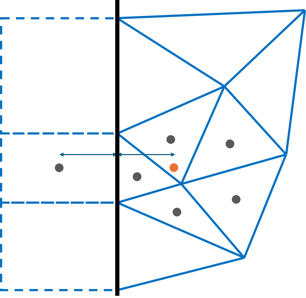
Here, if we want to get the centroid value for the ghost cell shown (I have left the other ghost cells at the top and bottom empty), then we see that the point on the other side of the boundary in the fluid domain would be where the orange dot is located. However, this point does not coincide with any centroid within the fluid domain, so we would have to get this point with an interpolation from surrounding points. This can be done, but higher-order schemes using ghost cells now would be limited by this second-order interpolation.

I have just shown one layer of ghost cells here, but for higher-order numerical schemes on unstructured grids, your stencil will be much larger. That means that we have to construct even more ghost cells. You see, on unstructured grids, the complexity quickly escalates, but we are not really gaining anything. We have to resort to second-order interpolation, so our higher-order scheme would lose accuracy near the boundaries anyway. It is simpler to just use a lower-order scheme here, which likely has the same accuracy but less computational cost.

Derived boundary conditions

Up until this point, we have only really touched upon Dirichlet-type and Neumann-type boundary conditions, as well as Robin-type as a combination of the two. This is really all that you need. If you are working with OpenFOAM, for example, you have countless of boundary conditions to choose from, but if you know these three fundamental types of boundary conditions, you can set up any flow problem.

If you are going for a commercial solver, they typically want to make your life as easy as possible and don’t have you think about what is Dirichlet and what should be Neumann. Instead, they provide abstract versions of these, which you will know under names such as Inlet, Outlet, Walls, Symmetry, Periodic or Cyclic, and so on.

So in this section, I want to shine a light on these boundary conditions and show what type of boundary conditions are actually solved here in terms of Dirichlet and Neumann. This can also help you write your own solver so you know what type of boundary conditions to impose in terms of Dirichlet and Neumann.

Solid boundary conditions

The first boundary condition we want to look at is solid boundary conditions. These are boundary conditions where flow cannot penetrate through the boundary, and typically, when we talk about solid boundary conditions, we refer to walls. But there are different types of wall boundary conditions, so let’s review them here.

Wall

The first type is the wall itself. We have already briefly discussed it before, but for completeness, I want to introduce it again here. At the wall, the velocity has to come to rest, and this means that all velocity components have to be zero for a stationary wall or the same speed as the wall if it is moving. The pressure develops at the wall, so we don’t know its values before we run the simulation, so we cannot impose the pressure here.

If we are dealing with the energy equation as well, that is, we are solving for the temperature, then we have two options. We can either set a constant temperature T or impose a heat flux. If the heat flux is set to zero, we have an adiabatic system (no heat is transferred between our fluid and the wall itself). Depending on our sign convention, we may have heating for a positive heat flux or cooling for a negative heat flux.

We can summarise a wall boundary condition as:

• Velocity: Dirichlet, with u=v=w=u_{wall}. For stationary walls, we have u_{wall}=0
• Pressure: Neumann, with \partial p/\partial n=0
• Temperature:
  • Dirichlet for constant temperature
  • Neumann for adiabatic walls with \partial T/\partial n=0
  • Neumann for heating with \partial T/\partial n>0
  • Neumann for cooling with \partial T/\partial n<0

Symmetry

The symmetry condition can be somewhat confusing. Yes, if we mirror the flow at the symmetry plane, we get a mirror image of the flow. But that is also true for all other boundary conditions, so this is not a very effective name in my view. Instead, I find it best to think of symmetry boundary conditions as a frictionless wall or a slip wall.

Essentially, a symmetry boundary condition is a solid wall as well, so no fluid can penetrate through it, with the exception that the velocity in the parallel direction of the symmetry boundary plane is treated as a Neumann boundary condition rather than a Dirichlet boundary condition. This means that we have

• Velocity: Dirichlet for \mathbf{u}_\perp=0 and Neumann for \partial\mathbf{u}_\parallel/\partial \mathbf{x}_\parallel=0. Here, \perp and \parallel are the normal and parallel direction at the boundary. We used n before to denote the normal direction at the wall, which is equivalent to the \perp direction, and \parallel is tangential/parallel to the symmetry boundary face.
• All other variables: \partial\phi/\partial n=0

Open boundary conditions

Open boundary conditions start to break things and will cause you headaches. As a general rule, place these boundaries as far away as possible from any object of interest so that they do not influence the flow near that object. If you can’t do that, then check that your open boundaries do not adversely influence the results.

Periodic or cyclic

These are the simplest open boundaries to implement. Assuming that your domain does indeed feature a periodic pattern, and it is suitable to consider just one instance and replace the boundaries with periodic boundaries, then these open boundary conditions are the only ones that will not adversely affect your simulation.

It is a popular boundary condition for turbulent flows, where we say that whatever goes out on one side of the domain has to go in on the opposite side of the domain. This requires that boundaries are parallel to each other and flat.

Let’s consider a simple example of a 1D case to see how we can implement them. You will have two boundaries, one on the left side and one on the right side. Let’s say that we have 10 vertices (finite difference) or 10 cells (finite volume), and let’s write the number of cells with the variable N=10. Then, we can establish the following index:

i\,\%\,N

Here, \% is the modulo operator, which will return the remainder of the division of i/N. For example, 5%10=5. 5/10=0 with a remainder of 5. Or take another example, 5%2=1. We can divide 5 by 2 exactly two times, this leaves a remainder of 1. So how does it relate to periodic boundary conditions?

Let’s consider the 1D heat diffusion equation with explicit time integration, This can be written as:

T_i^{n+1}=T_i^n+\alpha\frac{T_{(i+1)\%N}^n-2T_i^n+T_{(i-1)\%N}^n}{\Delta x^2}

Here, instead of T_{i+1}^n and T_{i-1}^n, I wrote T_{(i+1)\%N} and T_{(i-1)\%N}. We said that N=10, so let’s see what happens for i=8. We have 8%N=8%10=8; 10 does not fit into 8, so we have a remainder of 8. So (i+1)\%N=(8+1)\%10=9\%10=9. Similarily, (i-1)\%N=7. So these two statemets still return T_{i+1} and T_{i-1}, respectively.

This only becomes important at the boundaries. So let’s set i=N=10. We are now on the boundary vertex/cell, and we know there is no more vertex/cell to the right. Thus, i+1=10+1=11 does not exist as a location, as we only have N=10 vertices/cells. But, if we evaluate now (i+1)\%N, we get (10+1)\%10=11\%10=1. 11 divided by 10 is 1, with a remainder of 1.

On the left boundary, we have a similar situation. Here, we have (i-1)\%N=(0-1)\%10=-1. Hmm, that looks strange. The location i=-1 does not exist and is beyond the left side of the domain. There are two ways to deal with this. We can check each index and then add N whenever we have a negative number. In this case, we would have -1+N=-1+10=9, which is the vertex/cell one unit to the left on the right boundary.

Alternatively, we can also simply add N to all of our stencils. For example, in the previous example, we would modify this to (i-1+N)\%N=(0-1+10)\%10=9\%10=9. For the example on the right boundary, we would get (i+1+N)\%N=(10+1+10)\%10=(21)\%10=1. In the last case, we still get 1. Even though we added N, it doesn’t change the result, as the modulo operator \% returns the remainder, not the actual result of the division. The remainder will not change if we add multiples of N.

So, by using the modulo operator, we can simply implement boundary conditions without even being aware that they are there. While we haven’t used Dirichlet-type or Neumann-type boundary conditions here explicitly, since we are setting values beyond the boundaries to know values, periodic boundary conditions can be understood to be of type Dirichlet for all quantities that we are solving for.

Differences in open boundary conditions based on the Mach number

No all boundary conditions are created equal. Depending on the local Mach number, the flow’s behaviour will change. For example, for subsonic flows where the Mach number is below one, the pressure behaves in an elliptic manner, meaning that pressure disturbances are instantaneously propagated through the domain. This allows streamlines to start curving away from objects like airfoils before the flow has even reached these objects.

Once we go supersonic, the behaviour of the Navier-Stokes equation changes, and we get a hyperbolic behaviour. Now there is a defined direction of travel, and the pressure, for example, is no longer propagating instantaneously. So, for the airfoil example, it will only see the airfoil when it reaches it, causing an instant shock wave to form at the leading edge (depending on the shape of the airfoil, or in general, of the object, we may get a detached bow shock instead).

Since the behaviour of the flow changes as we go from subsonic (Ma<1) to supersonic (Ma\ge 1), so does the behaviour on the boundary, and so we need to account for that in our boundary conditions. In general, we have the following requirements on open boundaries for subsonic flows (Ma< 1):

• Inlet:
  • All boundary conditions are known and imposed as Dirichlet-type boundary conditions except for one.
  • One boundary condition needs to be of type Neumann.
• Outlet:
  • All boundary conditions are unknown and imposed as Neumann-type boundary conditions except for one.
  • One boundary condition needs to be of type Dirichlet.

In contrast, for supersonic boundaries (Ma\ge 1), we have:

• Inlet:
  • All boundary conditions are known and imposed as Dirichlet-type boundary conditions.
• Outlet:
  • All boundary conditions are unknown and imposed as Neumann-type boundary conditions.

The reason this changes has to do with the characteristics of the flow. They change their behaviour on open boundaries as the flow changes from a mixed-elliptic hyperbolic (subsonic) flow to a fully hyperbolic (supersonic) flow.

For subsonic (e.g. incompressible) flows, all but one characteristics are pointing into the domain. We impose values for these using Dirichlet-type conditions, but there is one characteristic that points outwards, and so we don’t know its value, and we have to impose that as a Neumann-type boundary condition. At the outlet, all but one characteristics point outwards, so we impose Neumann for them and one characteristic points into the domain, so we impose a Dirichlet type for it.

For supersonic (e.g. compressible) flows, this changes to all characteristics either pointing into the domain at the inlet, so we apply Dirichlet-type boundary conditions to all variables, or out of the domain at the outlet, so we apply Neumann-type boundary conditions to all variables.

We’ll have to keep this in mind for the remaining discussion, as boundary conditions will slightly change for the type of flow we have at hand.

Freestream or farfield

Having gone through the above discussion, we are going to discuss an exception immediately. Freestream or farfield conditions are fully Dirichlet-type conditions. That is, we set values for all variables at both the inlet and the outlet. How can we do that? Well, consider an aircraft flying in cruise condition. If we wanted to model this, and we placed a domain around the aircraft that is, say, 10 km wide in each direction, we can probably assume that if we are far enough away from an object in an external flow scenario, we have reached atmospheric conditions.

For example, the wake of the aircraft may have dissipated into heat and is no longer there, while the flow near the outlet will have returned to its original state. So if we place the boundaries very far away from the object that we are investigating, then farfield boundary conditions are not a bad starting point. This implies that we have open boundaries on all sides, i.e. we can’t use freestream or farfield boundary conditions for internal flows.

They are popular for aeronautical cases, e.g. airfoils, aircraft, and similar applications. But these are the exception to the rule, and, due to their requirement of no solid boundaries in the farfield, we can only use them for specific applications. If we want to have a more general open boundary condition, then we need to treat inlets and outlets separately so we can account for incoming and outgoing characteristics.

For completeness, let’s write out the boundary conditions. We have for both inlets and outlets:

• Velocity: Dirichlet
• Pressure: Dirichlet
• Temperature: Dirichlet

Pressure or velocity inlet

The pressure or velocity inlet, as the name suggests, specifies a value for either the pressure or velocity. This is imposed as a Dirichlet boundary condition. If we are dealing with an incompressible flow, we only need to consider the velocity and pressure, and we remember from our discussion above that for subsonic flows (all incompressible flows must be subsonic by definition), we need to specify at least one Neumann-type condition. For compressible flows, we have to specify Dirichlet-type boundary conditions everywhere.

We typically specify the velocity if we want to achieve a certain flow rate or Reynolds number. A pressure inlet, on the other hand, is typically used with a pressure outlet, where we specify a pressure gradient between the inlet and outlet. By knowing the length of the domain L_{domain}, we can compute the pressure gradient \nabla p as \nabla p=(p_{inlet}-p_{outlet}/L_{domain}).

Thus, for an incompressible flow, we impose the following conditions for a velocity inlet:

• Velocity: Dirichlet for all velocity components u, v, and w.
• Pressure: Neumann, typically \partial p/\partial n=0.
• Temperature: Either Dirichlet if the temperature at the inlet is known or Neumann if it is unknown.

For an incompressible flow, we impose the following conditions for a pressure inlet:

• Velocity: Neumann for velocity normal to inlet, i.e. \partial u_{\perp}/\partial x_\perp=0, Dirichlet for all tangential velocities, i.e. u_\parallel=0.
• Pressure: Dirichlet
• Temperature: The same as for the velocity inlet, Dirichlet if temperature is known, Neumann if it isn’t.

For a subsonic, compressible flow, i.e. Ma<1, we can impose either a velocity inlet or pressure inlet boundary condition as seen above. For a supersonic, compressible flow, i.e. Ma\ge 1, we impose the following conditions at the inlet:

• Velocity: Dirichlet
• Pressure: Dirichlet
• Temperature: Dirichlet

We do not differentiate between velocity and pressure inlets for compressible flows as all characteristics point into the domain. Thus, all quantities have to be specified.

Pressure or velocity outlet

The pressure or velocity outlet is the opposite to the corresponding inlet, in many ways, i.e. we prescribe either one velocity component or the pressure at the outlet, at least for incompressible flows. For compressible flows, we would specify Neumann-type boundary conditions for all variables.

For incompressible flows, we need to be careful with the pairing of inlets and outlets as well. If we use a velocity inlet, for example, we specify Neumann-type boundary conditions for the pressure. If we now also set the outlet to a velocity outlet, then we use Neumann-type boundary conditions again for the pressure. If we now have some walls as well in the domain, then we have further Neumann-type boundary conditions for the pressure. This is a problem.

Why? Well, we saw before that Neumann-type boundary conditions really just copy values from the internal domain and they set them at the boundaries. If all of our boundaries use a Neumann-type boundary condition, then the pressure is allowed to increase without bounds (and it will). In order to avoid this issue, we typically have to specify the value of the pressure in one cell, and then we ensure that this pressure is set for this one cell. In this way, we fix the pressure not through boundary conditions but instead through a single cell or a volume condition.

To avoid this issue, we can simply pair a velocity inlet with a pressure outlet, where we prescribe, for example, the ambient pressure at the outlet as a Dirichlet-type boundary condition. This is a common combination if we are using a velocity inlet. If we use a pressure inlet, we can still use a pressure outlet, as we prescribe now both pressure values as a Dirichlet-type boundary condition.

Thus, for an incompressible flow, we impose the following conditions at the velocity outlet:

• Velocity: One component Dirichlet, typically the velocity component normal to the boundary face, the remaining components are Neumann
• Pressure: Neumann
• Temperature: Neumann

For an incompressible flow, we impose the following conditions at the pressure outlet:

• Velocity: Neumann for all velocity components
• Pressure: Dirichlet, typically ambient pressure
• Temperature: Neumann

For a subsonic, compressible flow, i.e. Ma<1, we can either impose a velocity outlet or pressure outlet as seen above. For a supersonic, compressible flow, i.e. Ma\ge 1, we impose the following conditions at the outlet:

• Velocity: Neumann
• Pressure: Neumann
• Temperature: Neumann

I should mention here that, while technically possible, the velocity outlet is rarely used. It does have the issue of potentially having a fully Neumann-type boundary condition for the pressure, and thus, the pressure outlet is typically preferred.

Advective outlet

Thus far, we have only really discussed one type of boundary condition at the outlet, i.e. a combination of Dirichlet and Neumann boundary conditions. But in specific cases, we can impose a third type (or fourth, if you want to count Robin-type boundary conditions as well). This is to solve an advection equation at the outlet. In particular, this is the equation we are solving for the outlet:

\frac{\partial \phi}{\partial t}+u_\perp\frac{\partial \phi}{\partial n}=0

Here, u_\perp is the normal velocity at the outlet, and \partial \phi/\partial n is the derivative of \phi (velocity, pressure, temperature, etc.) at the outlet and it is normal/perpendicular to the boundary face. If we discretise this equation with a finite-difference approximation, for example, we have:

\frac{\phi^{n+1}_{i}-\phi_i^n}{\Delta t}+u_i^n\frac{\phi_i^n-\phi^n_{i-1}}{\Delta x}=0

Here, I have used a backward approximation for the derivative. Let’s assume that the vertex on the boundary is located at location i, so that location i-1 is on the internal fluid domain. If the boundary was located on the left side of the domain, then we would use a forward derivative in space, which we would evaluate at locations i and i+1, respectively.

If we solve this equation now for \phi_i^{n+1}, we get:

\phi_i^{n+1}=\phi_i^n-u_i^n\frac{\Delta t}{\Delta x}\left(\phi_i^n-\phi^n_{i-1}\right)

Thus, by knowing the values of \phi_i^n and the velocity normal at the boundary u_i^n from the previous time step (or the values obtained from the initialisation if it is the first time step), we can compute the values for \phi_i^{n+1} for the next time step.

You might be asking yourself, why would we go through the trouble of doing this? Well, the outlet conditions we have discussed in the previous section are so-called reflective boundary conditions, while the advective type discussed in this section are so-called non-reflective type boundary conditions. They do pretty much what their name suggests, but I think a video that shows both types in action will likely be more explanatory. Can you guess which type was used for the top and bottom domain?

Here, we see some pressure waves being advected by the flow. The top domain uses a pressure outlet of some sort (reflective), while the bottom domain uses an advective outlet (non-reflective).

Using one or the other will depend on your given flow problem. Reflective boundary conditions can sometimes lead to slower convergence, though this may be necessary to properly simulate the elliptic nature of the pressure. This, in turn, can influence the simulations and produce correct physical results that may not be obtained with an advective-type outlet condition, even though convergence may be accelerated.

Generally speaking, since all characteristics point outwards for compressible, supersonic flows, advective boundary conditions can be used here to ensure that no flow is entering back into the domain. This aligns with the physical expectation of a hyperbolic flow, and thus, correct physics can be reproduced while convergence may also be accelerated.

If this boundary condition is used for compressible flows, we can replace the normal velocity component u_\perp with the largest eigenvalue given by u_\perp + a, where a is the speed of sound.

Mass-based or volume-based inlets and outlets

Finally, we can also compute the inlet or outlet velocity by imposing a specific mass or volume flow rate. The volume flow rate can be computed as

\dot{V}=u_\perp\cdot A

Here, u_\perp is again the velocity component normal/perpendicular to the boundary, while A is the surface area of the boundary. This will give us a flow rate in units of m^3/s. For an incompressible flow, where the density remains constant, this is a good boundary condition, but for compressible flows, we may want to bring in the density as well. If we multiply the volume flow rate by the density, we get:

\dot{m}=\rho \cdot u_\perp\cdot A

This will give us a mass flow rate at either the inlet or the outlet. If the volume flow rate is given in units of m^3/s, multiplying this by the density gives us (m^3/s)(kg/m^3)=kg/s. Because of this unit, we call it the mass flow rate.

We can modify both the volume flow rate and the mass flow rate to the following equation:

u_\perp = \frac{\dot{V}}{A}\\[0.5em]
u_\perp =\frac{\dot{m}}{\rho \cdot A}

Thus, if we want to impose a volume or mass flow rate, we really just specify the velocity again as a Dirichlet boundary condition. This has some advantages and disadvantages.

The disadvantage is that we now potentially get a fully Neumann-type boundary condition for the pressure if we deal with subsonic speeds. This is typically the case, as volume flow rate and mass flow rate boundary conditions are typically used for internal flows, such as the flow through pipes and channels, which are rarely supersonic. So we have to use our little trick again of fixing the pressure in one cell to a specific value, i.e. we impose a volume condition for the pressure.

The advantage, however, is that by imposing a mass flow rate and using this boundary condition exclusively for open boundaries, we can ensure that mass is conserved in our domain. What goes in has to leave, and this means our continuity equation will be happy and converge, potentially, better.

Now, if we do not use mass flow rate boundary conditions and opt for a combination of velocity inlets and pressure outlets, there is no guarantee that we will conserve mass in our domain. If we are using an unstructured grid with tetrahedron or polyhedron elements, then we are inducing numerical diffusion. Combining that with a low-order upwind-based scheme, we will diffuse the results even further. This will artificially slow down the flow, and this leads to a reduced velocity at the outlet, which will not conserve mass.

So, the remedy here is that we simply look at the ratio of the computed mass flow rate at the inlet and outlet and multiply the velocities at the outlet by that value. This can be given as:

\dot{m}_{in}=\rho \cdot u_{in}\cdot A\\[0.5em]
\dot{m}_{out}=\rho \cdot u_{out}\cdot A\\[0.5em]
r_m=\frac{\dot{m}_{in}}{\dot{m}_{out}}\\[0.5em]
u_{out, corrected}=u_{out}\cdot r_m

The first three equations here are computed once (i.e. we compute the mass flow rate once at the inlet, once at the outlet, and we compute the ratio once). We then use this ratio to compute a corrected outlet velocity u_{out, corrected}. In this way, we ensure mass is conserved.

So, regardless of which boundary condition pairing we are using, we run into trouble. Pure velocity inlet and outlet conditions, such as those given by the mass flow inlet and outlet, result in a fully Neumann-type boundary condition for the pressure, and we have to fix the pressure through other means. A combination of velocity inlet and pressure outlet will avoid the issue with the pressure, but we now have to start adjusting the mass flow rate through velocity scaling.

For completeness, the boundary conditions for a mass or volume flow inlet are given as:

• Velocity: Dirichlet (see equations above for how to calculate the velocity)
• Pressure: Neumann
• Temperature: Dirichlet or Neumann, depending on whether a constant temperature should be imposed or if the temperature is unknown at the inlet.

At the outlet, we would impose the following conditions:

• Velocity: Dirichlet (again, see equations above for how to calculate the velocity)
• Pressure: Neumann
• Temperature: Neumann

While we could also state the boundary conditions for a supersonic compressible flow (i.e. fully Dirichlet at the inlet and fully Neumann at the outlet), I’ll refrain from doing so, as I can’t really think of an application where this would be useful. If you know of an application, let me know, and I’ll happily change the text here.

In the end, open boundaries will always pose some challenges, and our choices can have a noticeable influence on the results. We always need to verify that our boundary conditions are doing what we want them to, and a lot of issues with simulations can be traced back to incorrect boundary conditions. I think you get the point; I’ll leave it at that!

Summary

You survived my boundary condition rant. Congratulations. We started by looking at some of the challenges we face with boundary conditions, in particular with open boundary conditions. Then, we reviewed the three fundamental types that exist: Dirichlet, Neumann, and Robin-type boundary conditions. We also looked at the two different ways to implement them, either through no mesh modification or using ghost cells.

We then put that theoretical knowledge into practice. We reviewed derived boundary conditions, such as solid walls, symmetry planes, and various inlets and outlets, along with some modelling issues that we face based on how we want to treat our open boundary conditions.

Boundary conditions only get more complicated as we increase the modelling complexity. The more we want to resolve, the more unknown quantities we have to prescribe at the inlet for which we typically don’t have any reasonable values or estimates at hand. Scale-resolved turbulence modelling is the prime example here. Imposing physically correct fluctuations at the inlet for Large-eddy Simulations (LES) and Direct Numerical Simulations (DNS) are still unsolved questions, even though some progress has been made here.

If you experience convergence issues and you are happy it is not due to your mesh, then check your boundary conditions. Is there a way to improve them? Do you understand all the options your solver exposes here, and could you tweak them to make your boundary conditions align better with the case you are solving? Be critical of your boundary conditions, and your simulations will improve!

---

Tom-Robin Teschner is a senior lecturer in computational fluid dynamics and course director for the MSc in computational fluid dynamics and the MSc in aerospace computational engineering at Cranfield University.