Explicit vs. Implicit time integration and the CFL condition
When setting up a simulation and running it as an unsteady simulation or even just a steady state simulation with pseudo time stepping, we need to decide if we want to use explicit or implicit time stepping. The choice will have consequences down the line, and we need to be aware of them.
In this article, we will not just look at the differences between explicit and implicit time integration but also look at the two different types of CFL numbers that help us to quantify stability. We will see that explicit schemes are conditionally stable while implicit schemes are unconditionally stable. We will derive the equations to show why that is the case and then spend some time developing an intuition as to why we have these constraints.
We also look at how different time-stepping techniques can help us to really accelerate convergence beyond insanity, and once you finish the article, you'll have a profound understanding of explicit and implicit methods, as well as how they relate to the CFL number.
In this series
[custom_category_posts_list category_slug="10-key-concepts-everyone-must-understand-in-cfd"]In this article
- Introducing explicit and implicit time integration
- How to measure stability: von Neumann stability analysis
- A graphical representation of explicit and implicit methods
- Time-stepping techniques
- Applications for explicit and implicit time integration
- Summary
Introducing explicit and implicit time integration
It is entirely possible to use a commercial or open-source CFD solver without ever having to think about what time integration technique to select. Use the default time integration scheme and see if your simulation breaks. If it doesn't, great, continue until it does. As the saying goes, never change a running system (apparently, there is a Wikipedia entry for this, cool).
But you are probably here to get some clarity on what the difference is, and you probably want to know when to use which. So, let me give you an idea of what the main difference is. First of all, both explicit and implicit time integration refer to how we treat the time derivative in the Navier-Stokes equations (or, for that matter, in any other partial or ordinary differential equation).
Explicit time integration is only stable for relatively small time steps, and the time step size is directly tied to your mesh size. As you increase the number of cells (the local mesh spacing decreases for each cell), your time step also has to reduce. Thus, your computational efforts do not scale linearly but rather exponentially. Have a look at the following table, showing the number of cells, the corresponding max allowable time step, and time to reach the final solution:
| Number of cells | max allowable time step size [s] | Time to solution [hours] |
| 600 | 0.21 | 0.0008 |
| 2,400 | 0.11 | 0.008 |
| 9,600 | 0.053 | 0.059 |
| 38,400 | 0.026 | 0.79 |
| 153,600 | 0.016 | 9.05 |
This is taken from a 2D simulation. We can see that the number of cells is increased by a factor of 4 each time, meaning that we refine the mesh in each direction uniformly (by dividing the mesh spacing [katex]\Delta x[/katex] and [katex]\Delta y[/katex] by 2). As we do that, the max allowable time step steadily decreases by a factor of two. Thus, if we want to run the simulation on each grid for the same amount of simulated time, we need more time steps to reach this time. This is why the time to solution increases exponentially.
Contrast this with implicit time integration. Here, there is no maximum allowable time step, and you can use as large a time step as you want. You only need to make sure that your time step is small enough to still resolve the frequencies you are interested in. Say you are investigating some form of periodic motion, for example, the vortex shedding around a cylinder, as shown below:
You need to ensure that your time step is small enough so that you capture this periodic motion. If you set your time step larger, then your simulation will still be stable, but you may run into convergence issues, and certainly, the results will not be time-accurate (at best, you can hope for some form of time-averaged solution).
Implicit methods are, however, mathematically more complex and require the solution of a linear system at each time step. Thus, for each time step, we need to solve the system [katex]\mathbf{Ax}=\mathbf{b}[/katex]. The name linear system also suggests that we need, well, a linear equation. The Navier-Stokes equations aren't linear at all, and thus, we need to linearise them before we can use implicit methods.
Well, I should say that you can also restore the non-linear behaviour using implicit methods. But, to achieve that, you need to solve a Newton-Raphson method within each time step, where you solve [katex]\mathbf{Ax}=\mathbf{b}[/katex] within each Newton-Raphson iteration (i.e. several times for each time step). The cost this requires isn't worth the pain, so you practically won't find anyone working on that (well, a handful have made it their research focus; let us wish them well on their journey to Valhalla and return to reality).
Some people (possibly those trying to justify a Newton-Raphson approach?!) are arguing that even explicit methods are linearised (while others insist that it is fully non-linear). In the end, what you believe depends on the type of schemes you use and the experience you have with them. At least, this is from what I can observe. Why make arguments rooted in maths when you can loudly proclaim your beliefs? After all, we are doing religion, sorry, I meant to say science, after all ...
So, let's look at an equation to get some clarity. We will discretise the 1D Burgers equation, which serves as a model equation to showcase explicit and implicit time integration. The Burgers equation in 1D is given as:
\frac{\partial u}{\partial t}+u\frac{\partial u}{\partial x}=0We previously looked at how to discretise this kind of equation, so I won't go into much detail here again. I am using the same notations here as I did in the above-linked article, so if there is anything unclear, you may want to give it a quick read. We can write our discretised equation, using the finite-difference approximation and a central scheme, as:
\frac{u^{n+1}_i-u^n_i}{\Delta t}+u\frac{u^*_{i+1}-u^*_{i-1}}{\Delta x}=0A central scheme isn't a good idea for various reasons, but for the moment, we only care about the difference between explicit and implicit methods, so bear with me. We now need to specify at which time level we want to evaluate [katex]\partial u/\partial x[/katex], i.e. what time level we want to evaluate [katex]u^*[/katex] at. For an explicit method, we set [katex]u^*=u^n[/katex], and for an implicit method [katex]u^*=u^{n+1}[/katex]. Thus, we can write:
- Explicit time integration:
\frac{u^{n+1}_i-u^n_i}{\Delta t}+u\frac{u^n_{i+1}-u^n_{i-1}}{\Delta x}=0- Implicit time integration:
\frac{u^{n+1}_i-u^n_i}{\Delta t}+u\frac{u^{n+1}_{i+1}-u^{n+1}_{i-1}}{\Delta x}=0So, the difference is at which time level (the current time level [katex]n[/katex] or the next one at [katex]n+1[/katex]) we are evaluating the quantities in the spatial derivatives. Using an explicit time integration, we end up with a single velocity being evaluated at [katex]n+1[/katex], thus, we can solve the equation for [katex]u^{n+1}_i[/katex] and calculate the solution at the next time level, well, explicitly. In this case, we would obtain:
u^{n+1}=u^n_i-u\frac{\Delta t}{\Delta x}(u^n_{i+1}-u^n_{i-1})The factor in front of the parenthesis [katex]u\Delta t/\Delta x[/katex] is known as the Courant-Friedrichs-Lewy, or CFL number. Thus, we could have also written the above equation as:
u^{n+1}=u^n_i-\mathrm{CFL}(u^n_{i+1}-u^n_{i-1})For the implicit equation, well, things get a bit more complicated. We need to arrange the equation in a form where all of the unknown velocities are kept on the left-hand side (by convention), and all known quantities are stored on the right-hand side. This allows us to write out the linear equation [katex]\mathbf{Ax}=\mathbf{b}[/katex]. This is somewhat more time-consuming, and if you want to see how this is done, then feel free to look at my article on how to discretise the heat diffusion equation with an implicit time integration.
Let's return, for a second, to the implicit equation:
\frac{u^{n+1}_i-u^n_i}{\Delta t}+u\frac{u^{n+1}_{i+1}-u^{n+1}_{i-1}}{\Delta x}=0We haven't said anything about the velocity [katex]u[/katex] in front of the second fraction. Is this velocity evaluated at [katex]n[/katex] or [katex]n+1[/katex]? Well, this goes back to our friends in Valhalla. If we set it to [katex]u^n[/katex], then we have linearised our system and can evaluate [katex]\mathbf{Ax}=\mathbf{b}[/katex] directly. But, we set it to [katex]u^{n+1}[/katex], then we have a fully non-linear system and need to use a Newton-Raphson method, requiring several evaluations of [katex]\mathbf{Ax}=\mathbf{b}[/katex] per time step.
Thus, it is widely accepted to say that if both velocities in the non-linear term are evaluated at the same time step, it is fully non-linear, and if they are evaluated at different time steps, it is linearised. Eventually, if we are seeking a solution to a steady state problem, we would expect the difference between velocities at different time levels to go to zero, thus justifying linearisation. But to some, this is sacrilege based on their beliefs, though I would advocate that beliefs have no place in science (again, it isn't a religion).
OK, so we now have a somewhat vague idea about what explicit and implicit methods are. What I want to show you in this article is the following: First, we will review why explicit methods have a maximum allowable time step and why implicit methods work fine regardless of the time step. We will see how this is linked to the CFL number introduced above. For this, we will use the von Neumann stability analysis, which is limited, yet rather popular and effective in determining the max allowable time step for explicit schemes.
Next, I want to show you graphically why explicit schemes are bounded in their time step while implicit methods aren't. We will then look at some specific time-stepping techniques and insights I have found over the years that aren't widely covered in books and other resources, but that will help you to understand the importance of time-stepping, and, finally, we will look at applications when we want to use explicit methods, and when implicit methods are required.
Sounds good? Cool, let's get started!
How to measure stability: von Neumann stability analysis
John von Neumann is, well, right up there with the greats in CFD (although the field, as such, did not exist back then). He was instrumental in developing concepts that would form the basis of computational science and, by extension, the foundation of CFD. He was working at Los Alamos during the second small disagreement (aka the Second World War) and was a consultant on the Manhattan Project (aka Let's Build an atomic bomb). In a sense, we have the Germans to thank for his development (of course, I wouldn't say that being a German myself ... (you are welcome, though))
During his time, he developed numerical tools to investigate explosions, and one of the things he needed to develop was a criterion that allowed him to determine a stable time step for his calculations. Since this was all part of the Manhattan Project, his work was classified, and then some idiots didn't know what classified meant and published his results anyway. To be fair, it was shortly after the second small disagreement ended (in 1947), so they can be forgiven?!
As it turned out, these idiots weren't quite so idiotic; they were Crank and Nicholson, famous for their own time integration technique. It sure is handy if you can get your hands on classified information, de-classify it without consent and use the knowledge to create your own time integration technique. It sounds a lot like insider trading, but hey, if this means we will get a Trump time integration scheme, then I'm OK with that.
OK, so what is this von Neumann stability analysis? I could say that it is rather straightforward, and it is, but that is the case for everything you know. To someone who has never seen the von Neumann stability analysis, it will feel rather strange and unintuitive, so let us start with an example.
The figure below shows the solution of a discretised equation with a theoretically infinite number of points. As the number of points goes to infinity (or the spacing between two grid points goes to zero), we expect to recover the exact solution of the discretised equation (not necessarily, though, of the governing equation, as boundary conditions, numerical schemes, and run-time models such as turbulence models influence the solution of the discretised equation).
If we are using a discretised equation with a finite number of mesh points, i.e. we have a certain number of grid points with a non-zero spacing between each grid point, then we will see some differences to the exact solution (exact in the sense that it has an infinite number of points and thus satisfies the discretised equation exactly) and the discretised numerical solution. This is shown in the figure below (you can ignore the boosted mode 1 line for the moment):
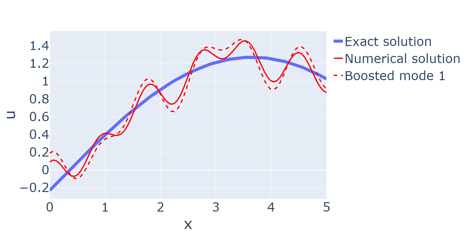
The difference between the exact discretised equation and the numerical solution on a grid with a finite number of points is now typically due to some round-off errors, as both equations use the same boundary conditions, numerical scheme, potential turbulence model, and so on. Sure, numerical dissipation also plays a role, but for grids that are fine enough, it will tend to go away. We would still expect some differences, which are now dominated by round-off errors. This is what we see in the figure above (granted, I have amplified the error here so we can see it more easily).
So, let's look at the error itself. This is shown in the figure below:
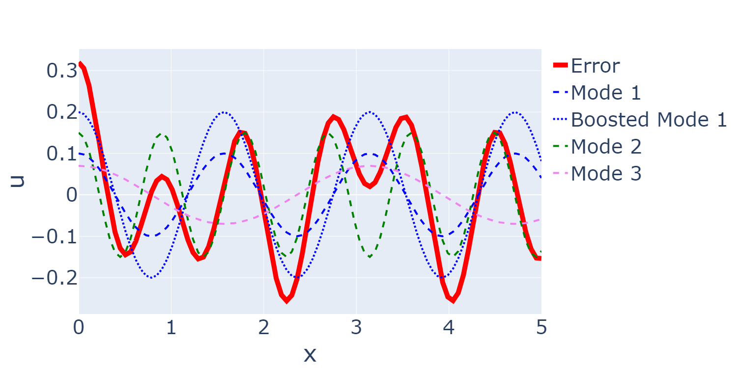
This error (shown in red) is obtained by subtracting the numerical solution from the exact solution. Looking at it, we can probably all agree that it has a certain wave-like behaviour. And what mathematical function do we use to represent such waves? Well, sine and cosine functions, right?
With this knowledge at hand, we could now throw a (Fast) Fourier Transformation (F)FT at the problem to get the frequency and amplitude of the waves that make up the error. And this is what I have done. There are three dominant waves described by a cosine function (or rather, modes, as they are called), which I have plotted in the figure as well (ignore the boosted mode for the moment again).
Thus, if you go anywhere in the graph on the x-axis and add up the values of all three modes, you get the value of the error shown in red. So, let's return to that boosted mode. What I have also done is to multiply the amplitude of the first mode by a factor of two. This is what we are seeing in the plot above. If you compare mode 1 with its boosted version, you see that it has the same frequency and just doubles its amplitude.
It is important to reiterate that mode 2 and 3 were left unchanged. Let's then inspect the error of the numerical solution compared to the exact discretised equation solution, which we saw in the figure before. We can see the numerical solution (which still has the error present) but now using the error composed of all three modes where the first mode is multiplied by a factor of 2. We can see that this numerical solution will have a larger error than the original signal, which is shown in solid red.
What does this mean for our current analysis? Well, we are interested in the stability of our numerical schemes. If the numerical solution should be stable, that means that our error should, at a minimum, not increase over time and, ideally, decrease as we advance the solution in time. Hopefully this makes sense, if the error were to increase over time, the numerical solution would become unstable and diverge, leading to a crash of your simulation.
And with that, we have all the ingredients we need to understand the von Neumann stability analysis. However, there are a few assumptions to make this stability analysis work.
First, we assume that the problem we are investigating has periodic boundary conditions. This is done so that our error can be non-zero at the boundaries. If we had an inflow, outflow, or a solid wall, for example, we would likely specify some Dirichlet boundary conditions (i.e. we would impose values at the boundary directly, such as the inflow velocity).
If we impose values at the boundaries, then we consider them exact, and if they are exact, then we don't have any errors at the boundaries. This would mean that all modes have to go to zero at the boundaries, but we don't have a mechanism to set a sine or cosine wave to zero at an arbitrary position, i.e. they will just behave as waves until they reach the end of the domain.
The second assumption von Neumann made is that the numerical solution for which we wish to seek a stability criterion is linear. This is a big simplification, as the Navier-Stokes equations are non-linear. However, as our time step becomes smaller and smaller, the changes from one time step to the next become smaller as well, and this small change may be reasonably well approximated by a linear assumption. As long as the solution is smooth, this works well, but once strong non-linear effects, such as sock waves, enter the picture, this changes.
The advantage of saying the problem is linear is that we can concentrate just on a single mode and see if it is increasing or decreasing over time. The linear assumptions assume that if one mode is increasing, the overall error must be increasing as well. Likewise, if the overall error is decreasing, then the overall error must decrease as well. This is what we saw above when we looked at what happens if we boost just a single mode (we saw the overall error increasing).
Finally, we said that if we are dealing with a wave-like pattern, such as seen in the error plot above, we can use the Fourier transform to obtain the dominant modes. We can expand this concept and say that any function that exhibits a wave-like behaviour can be approximated with a Fourier series of the form:
f(x)=\sum_{j=-\infty}^\infty A^n e^{I\theta_j x}Here, we have [katex]I=\sqrt{-1}[/katex], [katex]A^n[/katex] being the amplitude at time level [katex]n[/katex] and the phase angle [katex]\theta_j=k_j\Delta x[/katex], where [katex]k_j=2\pi/\lambda_j[/katex] is the wave number and [katex]\lambda_j[/katex] the wavelength. Think of [katex]\theta_j[/katex] as being related to the frequency if all these definitions are too much. In the error plot above, we saw that we had three separate modes (cosine waves) and mode 2 had a high frequency (short waves) while mode 3 had a high frequency (long wave).
Since we said that the overall error will increase if just one of the modes increases, we can concentrate on a single mode. This means we pick any of the [katex]j[/katex]-th mode and simply write [katex]\theta_j[/katex] as [katex]\theta[/katex]. Having said that, we can express the error now as follows:
\mathrm{error}(f(x))\propto A^n e^{I\theta x}We aren't interested in the exact error, we only care if the error is increasing or decreasing, thus it is sufficient to say that the error is proportional to the right-hand side.
General procedure in the von Neumann stability analysis
OK, so what have we gained? Well, we can now go into any discretised equation, replace the numerical approximation with a single Fourier mode seen above and then see if this error is increasing or decreasing. The steps are always the same:
- First, we replace the variables within our discretised equation with a single Fourier mode. This results in:
\phi_i^n=A^ne^{I\theta i}\\
\phi_{i\pm 1}^n=A^ne^{I\theta (i\pm 1)}=A^ne^{I\theta i}e^{\pm I\theta}\\
\phi_i^{n+1}=A^{n+1}e^{I\theta i}\\
\phi_{i\pm 1}^{n+1}=A^{n+1}e^{I\theta (i\pm 1)}=A^{n+1}e^{I\theta i}e^{\pm I\theta}
Thus, whenever we encounter [katex]\phi_{i\pm 1}^n[/katex] or [katex]\phi_{i\pm 1}^{n+1}[/katex], we replace it by the Fourier component above.
- We then require that the solution is stable if the error is not being amplified. Since [katex]A^n[/katex] is the amplitude of the error at time level [katex]n[/katex], we can define an error amplification factor [katex]G[/katex] as
G=\frac{A^{n+1}}{A^n}As long as we have [katex]|G|\le 1[/katex], we know that the error is decreasing (or at least not increasing, i.e. [katex]|G|=1[/katex]).
- Finally, we insert the definition for [katex]G[/katex] into our discretised equation and see under which condition this inequality is reaching its maximum, i.e. [katex]|G|=1[/katex]. Most of the time, this can be shown through equations, but a more convenient method is to plot the results in a complex number plane and then depict graphically under which condition stability is no longer attained.
Model equations to determine stable time-stepping conditions
In order to determine the maximum allowable time step, we need to apply the above-mentioned procedure to a discretised equation. Sure, we can throw that at the Navier-Stokes equation and then get a complex mess of a stability condition that isn't really intuitive. Instead, with far less complexity but with the same result, we can look at two model equations that represent the two fundamental properties of the Navier-Stokes equation.
These equations are the general diffusion equation and the linear advection equation. The diffusion equation will tell us what the stability requirement is for flows with low Reynolds numbers (e.g. Stokes flow, where we have [katex]Re\approx 1[/katex]). The linear advection equation, on the other hand, will tell us what the stability requirement is for high Reynolds number flows, i.e. [katex]Re>>1[/katex] (e.g. turbulent flows, in general).
We only consider the 1D version of each equation, but the results would be the same for 2D and 3D (just more mathematically involved, so let's stick to the simplified 1D version). The model equations are given as follows:
- General diffusion equation:
\frac{\partial u}{\partial t}=\Gamma\frac{\partial^2 u}{\partial x^2}- Linear advection equation:
\frac{\partial u}{\partial t}+a\frac{\partial u}{\partial x}=0We will see that explicit schemes are, at best, bounded by their CFL number, while implicit schemes do not have the same limitation. Before we investigate the stability of various numerical schemes on these equations, let us first review Euler's formula, as we will make heavy use of it.
Intermission: Euler's formula
Euler's formula allows us to map between complex numbers and trigonometric functions. Take the following unit circle plotted in the complex plane. We can express any point on this unit circle through a combination of sine and cosine values:
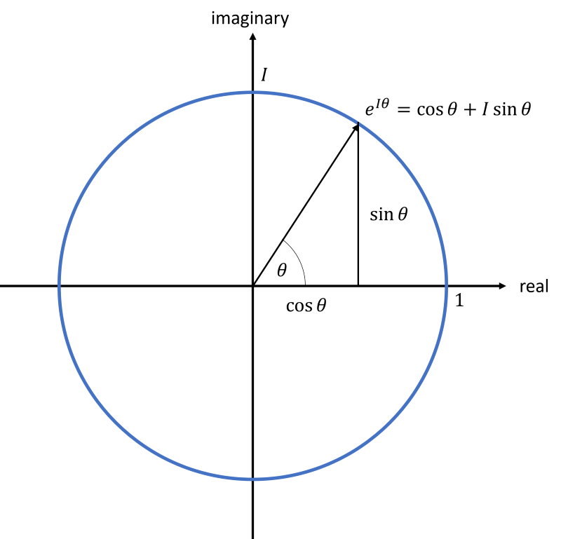
If you are afraid or uncomfortable with complex numbers (well, thinking about it, I don't know anyone feeling comfortable with complex numbers; 2D numbers are a strange concept!), see the above plot as a simple x-y plot and ignore the imaginary part, just think of it as the y-axis. If we wanted to find any value on a circle centred around the origin with a radius of 1, we would be able to find any point on this circle through a combination of sine and cosine values. This is just what Euler's formula is telling us in the complex plane as well, using complex number notation.
Thus, as we can see from the figure above, Euler's formula can be given as:
e^{I\theta}=\cos\theta+I\sin\thetaEqually, we can define the negated version as
e^{-I\theta}=\cos\theta-I\sin\thetaIn both cases, we have used [katex]I=\sqrt{-1}[/katex], i.e. we are dealing with complex numbers here. We can combine the two definitions above (either by adding or subtracting them from each other) to get definitions for [katex]\sin[/katex] and [katex]\cos[/katex] as follows:
\cos\theta=\frac{e^{I\theta}+e^{-I\theta}}{2}\sin=\frac{e^{I\theta}-e^{-I\theta}}{2I}These relations will be used in the following to derive stable time stepping conditions.
Example: Linear advection equation
The linear advection equation is probably one of the most studied model equations in CFD. It is rather straightforward to implement and understand, though, if you are seeing it for the first time, it can already be complex enough to keep you up a few nights (it certainly did that for me back in the day).
In this section, we will discretise the equation using a first-order upwind scheme using both an explicit and implicit time integration approach. We will then see by using the von Neumann stability analysis that explicit schemes are necessarily bounded by the CFL condition, but implicit schemes are not.
We will also look at the second-order central scheme, which is known to be unstable. We will see that the von Neumann stability analysis predicts this correctly, but we also see that an implicit formulation, in theory, provides stable results.
First-order upwind, explicit
Let's start with the discretised linear advection equation. It is given, for an explicit first-order upwind discretisation as:
\frac{u^{n+1}_i-u^n_i}{\Delta t}+a\frac{u^n_i-u^n_{i-1}}{\Delta x}=0Here, we assume that [katex]a>0[/katex]. Since this is an explicit time integration, i.e. apart from the time derivative, all other quantities are solved at time level [katex]n[/katex], we can solve this equation for [katex]n^{n+1}_i[/katex] directly and obtain:
u^{n+1}_i=u^n_i-a\frac{\Delta t}{\Delta x}(u^n_i-u^n_{i-1})=u^n_i-\mathrm{CFL}(u^n_i-u^n_{i-1})We can see the CFL number appearing in the discretised equation, i.e. [katex]\mathrm{CFL}=a\Delta t/\Delta x[/katex].
To deploy our von Neumann stability analysis, we first have to replace all [katex]u^n_{i}[/katex], [katex]u^{n+1}_i[/katex], [katex]u^n_{i-1}[/katex] variables with a single Fourier mode. Using the relations we derived above, we can insert them and obtain:
A^{n+1}e^{I\theta i}=A^{n}e^{I\theta i}-\mathrm{CFL}(A^{n}e^{I\theta i}-A^{n}e^{I\theta i}e^{-I\theta})Remember, introducing the Fourier mode here means we now have an equation which tells us how the error is behaving. This is the plot we saw a bit ago, where we decomposed the error into three modes. We are now only concerned with a single mode since if one (error) mode increases in amplitude (given by [katex]A[/katex]), then the overall error will increase as well (as we saw above with the first mode being boosted).
The above equation contains a common factor [katex]e^{I\theta i}[/katex] in all terms, so let's divide by that:
A^{n+1}=A^{n}-\mathrm{CFL}(A^{n}-A^{n}e^{-I\theta})Now we use our definition of the error amplification factor of [katex]G=A^{n+1}/A^{n}[/katex]. We need to divide the above equation by [katex]A^n[/katex], in order to introduce [katex]G[/katex] into the equation. Doing so results in:
G=1-\mathrm{CFL}(1-e^{-I\theta})Now, it is time to insert our relation from Euler's formula discussed above. We replace [katex]e^{-I\theta}[/katex] and obtain:
G=1-\mathrm{CFL}(1-\cos\theta+I\sin\theta)We now introduce our stability criterion; that is, we insist that [katex]|G|\le 1[/katex]. This results in two separate inequalities:
1-\mathrm{CFL}(1-\cos\theta+I\sin\theta)\le 1\\
1-\mathrm{CFL}(1-\cos\theta+I\sin\theta)\ge -1
The question becomes, for which CFL values do these inequalities hold true? Or, put another way, what is the largest CFL number that we can use to still satisfy these inequalities? Well, let us plot the results and then see for ourselves. To understand our results, we need to have clarity on how [katex]G[/katex] is supposed to look in a complex number plane, given that the above inequalities use complex numbers.
Since we said that to have stable results, we require that [katex]|G|\le 1[/katex], that means the max allowable value for [katex]G[/katex] is one. If we go into the complex number plane, this means that the value of [katex]G[/katex] has to be 1, but rather its magnitude. Thus, if we were to draw a complex number for different phase angles of [katex]\theta[/katex] where the magnitude is 1, we would end up with a unit circle centred on the origin, similar to the unit circle we saw above in Euler's formula.
Therefore, the error amplification factor [katex]G[/katex] is just a unit circle itself, and so, if we plot the above inequalities for different values of [katex]\theta[/katex], they all need to stay within this unit circle. If they don't, we know the error is being amplified, and our scheme is unstable in time.
The only parameter we can tune in the above inequalities is the CFL number, and so we can plot the inequalities for different CFL numbers until they touch, but not cross, the unit circle made up by [katex]G[/katex]. The complex number with a CFL number that touches this unit circle will have an error amplification factor of [katex]|G|=1[/katex]; thus, we cannot increase the CFL number.
This will be our max allowable CFL number, and thus, we can determine the max allowable time step from the definition of the CFL number as
\mathrm{CFL}=a\frac{\Delta t}{\Delta x} \quad\rightarrow\quad \Delta t_{max}=\mathrm{CFL}_{max}\frac{\Delta x}{a}Let's do that, then. The plot below shows the unit circle spanned by [katex]G[/katex], as well as the complex number [katex]1-\mathrm{CFL}(1-\cos\theta+I\sin\theta)[/katex] for [katex]\mathrm{CFL}=[0.25, 0.5, 0.75, 1][/katex].
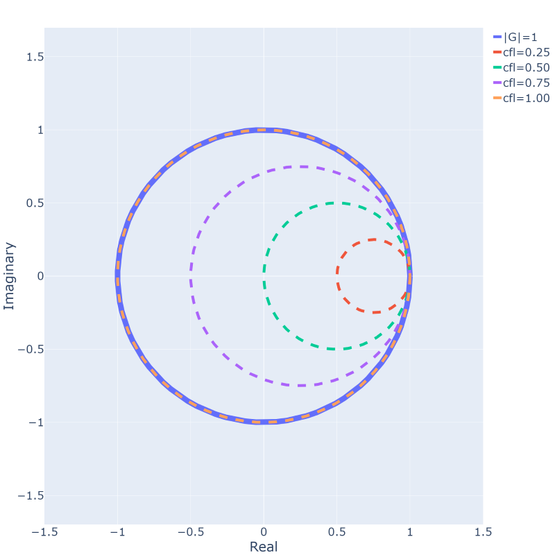
We can see that each CFL number combination is just creating a circle itself, and, for [katex]\mathrm{CFL}=1[/katex], both circles overlap entirely. Thus, graphically, we can show that [katex]\mathrm{CFL}_{max}=1[/katex] for the upwind scheme using an explicit time discretisation. This is termed conditional stability in the literature.
Let's see how this changes for implicit schemes.
First-order upwind, implicit
If we choose implicit time discretisation, we evaluate all of our velocities at time level [katex]n+1[/katex]. Using the same first-order upwind scheme as seen above, we can write our discretised equation as:
\frac{u^{n+1}_i-u^n_i}{\Delta t}+a\frac{u^{n+1}_i-u^{n+1}_{i-1}}{\Delta x}=0We solve for [katex]u^{n+1}_i[/katex] that we have within our time derivative (even though we also have a [katex]u^{n+1}_i[/katex] in our spatial derivative) and obtain a similar equation as for the explicit scheme seen in the previous section:
u^{n+1}_i=u^n_i-a\frac{\Delta t}{\Delta x}(u^{n+1}_i-u^{n+1}_{i-1})=u^n_i-\mathrm{CFL}(u^{n+1}_i-u^{n+1}_{i-1})At this point, we introduce our Fourier mode again. The only difference here is that since we used the velocities at time level [katex]n+1[/katex], the error magnitude will also be evaluated at the same time level, i.e. we have [katex]A^{n+1}[/katex]. This results in:
A^{n+1}e^{I\theta i}=A^{n}e^{I\theta i}-\mathrm{CFL}(A^{n+1}e^{I\theta i}-A^{n+1}e^{I\theta i}e^{-I\theta})=A^{n}e^{I\theta i}-A^{n+1}\mathrm{CFL}(e^{I\theta i}-e^{I\theta i}e^{-I\theta})Dividing this equaton again by the common factor [katex]e^{I\theta i}[/katex] results in:
A^{n+1}=A^{n}-A^{n+1}\mathrm{CFL}(1-e^{-I\theta})We can now insert the definition for the error amplification factor [katex]G[/katex] by dividing the equation by [katex]A^n[/katex]. This results in:
G=1-G\cdot\mathrm{CFL}(1-e^{-I\theta})Since we used an implicit time integration technique, we obtain a second [katex]G[/katex] on the right-hand side, and thus, we need to combine this with the error amplification factor on the left-hand side of the equation. This is achieved by simply adding it to the left-hand side and than factoring [katex]G[/katex] out.
G+G\cdot\mathrm{CFL}(1-e^{-I\theta})=G[1+\mathrm{CFL}(1-e^{-I\theta})]=1Now we can divide by [katex]G[/katex]'s factor given in the parenthesis, and we obtain:
G=\frac{1}{1+\mathrm{CFL}(1-e^{-I\theta})}Inserting the definition for [katex]e^{-I\theta}[/katex] from Euler's formula again, we arrive at:
G=\frac{1}{1+\mathrm{CFL}(1-\cos\theta+I\sin\theta)}Similar to the explicit case above, let us plot this complex number for different values. In this case, I have used [katex]\mathrm{CFL}=[1, 25, 50, 100][/katex] and the results for that are shown below:
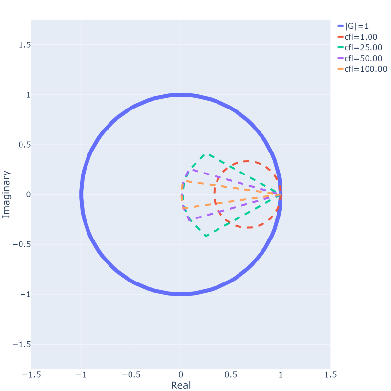
As the CFL number increases, the area mapped out by the complex number decreases, but it always stays within the complex unit circle spanned by [katex]G[/katex]. Thus, we can say that regardless of the CFL number, an implicit time integration scheme using a first-order upwind discretisation in space is always stable. In the literature, this is referred to as unconditional stability.
For a bit of fun (I know, I have a weird definition of fun), why not do the von Neumann stability analysis for the second-order central scheme in space, both explicit and implicit? Sounds god? Cool, let's give it a try as well.
Second-order central, explicit
By now, you know the drill. We first start with our discretised equation, which now uses a second-order central scheme in space and variables are evaluated at time level [katex]n[/katex]. Thus, the explicit formulation is given as:
\frac{u^{n+1}_i-u^n_i}{\Delta t}+a\frac{u^n_{i+1}-u^n_{i-1}}{2\Delta x}=0We solve this again for [katex]u^{n+1}_i[/katex] and obtain:
u^{n+1}_i=u^n_i-\frac{\mathrm{CFL}}{2}(u^n_{i+1}-u^n_{i-1})Inserting our Fourier mode results in:
A^{n+1}e^{I\theta i}=A^{n}e^{I\theta i}-\frac{\mathrm{CFL}}{2}(A^{n}e^{I\theta i}e^{I\theta}-A^{n}e^{I\theta i}e^{-I\theta})We divide this again by our common factor [katex]e^{I\theta i}[/katex] to get:
A^{n+1}=A^{n}-\frac{\mathrm{CFL}}{2}(A^{n}e^{I\theta}-A^{n}e^{-I\theta})=A^{n}-A^{n}\frac{\mathrm{CFL}}{2}(e^{I\theta}-e^{-I\theta})Inserting the error amplification factor by dividing this equation by [katex]A^n[/katex] results in:
G=1-\frac{\mathrm{CFL}}{2}(e^{I\theta}-e^{-I\theta})We saw from Euler's formula that we can express the brackets through a trigonometric relationship. Specifically, we saw:
\sin\theta =\frac{e^{I\theta}-e^{-I\theta }}{2I}\quad\rightarrow\quad 2I\sin\theta=e^{I\theta}-e^{-I\theta }We can insert this definition and obtain:
G=1-\frac{\mathrm{CFL}}{2}(2I\sin\theta)=1-I\cdot\mathrm{CFL}\sin\thetaNow, this is an interesting result. If we look at the imaginary and real part of this number, then we have [katex]Re=1[/katex] and [katex]Im=I\cdot\mathrm{CFL}\sin\theta[/katex]. This means that regardless of the CFL number, it will always be at 1 on the real (x) axis. Changing the CFL number would only change the value on the imaginary (y) axis, so we would expect to see a vertical line touching the unit circle tangentially at [katex]Re=1[/katex]. Let us plot this to verify this behaviour:
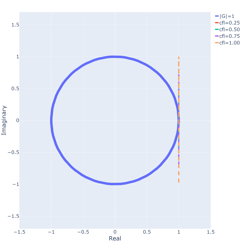
Indeed, we end up with a vertical line. Since we have [katex]Im=I\cdot\mathrm{CFL}\sin\theta[/katex], where [katex]\sin\theta[/katex] is clamped between -1 and 1, we see that the CFL number is simply scaling this range, i.e. if the CFL number is 1, then the range of the line plotted is from -1 to 1. If the CFL number is 0.75, the range is from -0.75 to 0.75, and so on.
This means that only in the limiting case of [katex]\mathrm{CFL}=0[/katex] do we obtain a stable numerical scheme, as the length of the line now reduces to a single point, which lies on the unit circle. However, a numerical simulation of [katex]\mathrm{CFL}=0[/katex] means that there is no flow. Consider the discretised equation again:
u^{n+1}_i=u^n_i-\frac{\mathrm{CFL}}{2}(u^n_{i+1}-u^n_{i-1})If we now say that the CFL number has to be zero, we end up with
u^{n+1}_i=u^n_i-\frac{0}{2}(u^n_{i+1}-u^n_{i-1})\quad \rightarrow\quad u^{n+1}_i=u^n_iThe simulation would converge to the initial conditions within one iteration, and thus, no meaningful results would be obtained. Thus, the literature labels the central scheme with explicit time stepping as unconditionally unstable. But things change if we use an implicit time discretisation. Let's review that in the next example as well.
Second-order central, implicit
Same old, same old, we start with the discretised equation:
\frac{u^{n+1}_i-u^n_i}{\Delta t}+a\frac{u^{n+1}_{i+1}-u^{n+1}_{i-1}}{2\Delta x}=0Solving for the velocity at time level [katex]n+1[/katex] within the time derivative, we get
u^{n+1}_i=u^n_i-\frac{\mathrm{CFL}}{2}(u^{n+1}_{i+1}-u^{n+1}_{i-1})Replacing velocities by a single Fourier mode to study the error amplification provides:
A^{n+1}e^{I\theta i}=A^{n}e^{I\theta i}-\frac{\mathrm{CFL}}{2}(A^{n+1}e^{I\theta i}e^{I\theta}-A^{n+1}e^{I\theta i}e^{-I\theta})We divide this again by our common factor [katex]e^{I\theta i}[/katex] to get:
A^{n+1}=A^{n}-\frac{\mathrm{CFL}}{2}(A^{n+1}e^{I\theta}-A^{n+1}e^{-I\theta})=A^{n}-A^{n+1}\frac{\mathrm{CFL}}{2}(e^{I\theta}-e^{-I\theta})Now we divide by [katex]A^n[/katex] again to see how the error propagates in time:
G=1-G\frac{\mathrm{CFL}}{2}(e^{I\theta}-e^{-I\theta})Solving for [katex]G[/katex] results in:
G-G\frac{\mathrm{CFL}}{2}(e^{I\theta}-e^{-I\theta})=1\\
G\left(1-\frac{\mathrm{CFL}}{2}(e^{I\theta}-e^{-I\theta})\right)=1\\
G=\frac{1}{1-\frac{\mathrm{CFL}}{2}(e^{I\theta}-e^{-I\theta})}
Using Euler's formula again with [katex]2I\sin\theta=e^{I\theta}-e^{-I\theta}[/katex], we obtain:
G=\frac{1}{1-\frac{\mathrm{CFL}}{2}2I\sin\theta}=\frac{1}{1-I\cdot\mathrm{CFL}\sin\theta}Ok, plotting time, how does this complex number look like?
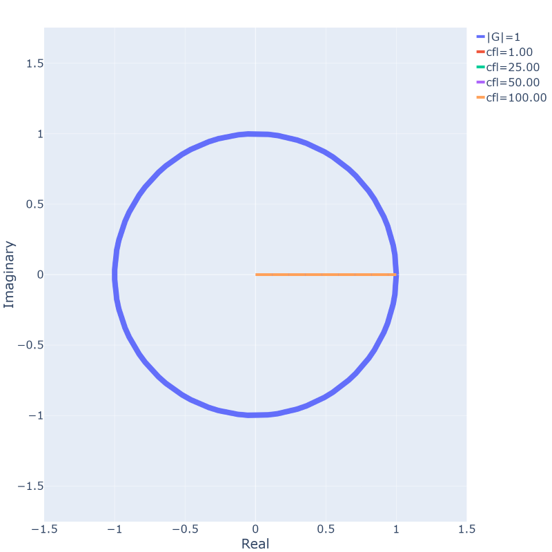
Well, the behaviour is such that we are always starting at [katex]Re=1[/katex] and then, depending on the CFL value, will get a line that spans from 1 to 0 on the real axis. It doesn't show well in the figure above, but if you plot the values yourself, you see that as the CFL number goes to zero, the line converges to a point at [katex]Re=1[/katex] and, as the CFL number increases to infinity, it reaches [katex]Re=0[/katex] as its maximum value.
Thus, an implicit central scheme is unconditionally stable. It is still not a super popular scheme, even though it shows stability. However, on grids where the local Peclet number is of the order of 1, it can be shown that even the explicit central scheme is stable and thus useful. As long as we are not dealing with strong shocks (or other discontinuous signals), the central scheme can be (and is!) used here. Typically, flows where the local Peclet number is around one is on grids with a very (very!) fine resolution. We are talking about large eddy simulations or direct numerical simulations.
And, if you must know, the Peclet number is just a ratio of the rate of advection and the rate of diffusion. This means that if we have a ratio of one, advection and diffusion are of equal strength. Likewise, if we have a Peclet number of infinity, this means we only have advection and no diffusion, while a Peclet number of 0 means pure diffusion. The article on Wikipedia has a nice animation for all three cases, so it is worth checking out if this is a new concept for you.
OK, so hopefully, by now, you agree that the von Neumann stability analysis isn't that complicated and that it follows a predictable pattern. If you look into the literature, then you will see actually a few more steps compared to what I have shown here. The reason I have not gone into all that much mathematical detail is that I remember being stuck on simplifying the equations when I was a student and learning about the von Neumann stability analysis. You may try to apply it now to your own schemes and get stuck as well if you try to get an elegant, simplified equation.
In the end, as long as you can get to an equation where you have [katex]G[/katex] on the left-hand side, you can then plot whatever is on the right-hand side and determine the stability bounds numerically (no need even to find a trigonometric expression for [katex]e^{\pm I\theta}[/katex]). This is far easier, and you can always impress your parents later with your complex number magic once the von Neumann stability analysis becomes second nature.
I think this should be sufficient for the linear advection equation. I want to look at pure diffusion as well, though, as stability changes here and this is often forgotten, so let us review this as well.
Example: Diffusion equation
The diffusion equation is another common example to study. Unlike the linear advection equation, the central scheme works really well here (if we piggyback off our discussion above, if we have pure diffusion, the local Peclet number will be 0, and thus, even the explicit central scheme is expected to work well here).
In CFD, it is really just the convective non-linear term in the Navier-Stokes equation that requires some attention, all the other terms work well with a second-order central scheme (well, the time derivatives are treated differently but we could use a second-order central scheme here as well).
As a reminder, the pure diffusion case is governed by the following model equation:
\frac{\partial u}{\partial t}=\Gamma\frac{\partial^2 u}{\partial x^2}In the literature, you likely see this more commonly expressed in terms of the temperature, i.e. [katex]u=T[/katex], but to keep the notation consistent with our linear advection equation, I have kept the velocity [katex]u[/katex] here. After all, we do have diffusion of the form shown above in the momentum equation.
We will review just the central scheme here and look at its stability condition for explicit and implicit time integrations. This is likely the only scheme you will ever come across for treating this term. Take it from me: I have implemented 8th-order accurate central schemes for the diffusion term, and I could barely see any difference to its second-order counterpart (of course, you may look at a specific problem where it may be useful. Implement and test it, and if it does make a noticeable difference, you can still cancel me).
Second-order central, explicit
We'll start with the usual steps. First, we create the discretised equation, which for the diffusion equation with a second-order central scheme for the diffusive term looks as follows:
\frac{u^{n+1}_i-u^n_i}{\Delta t}=\Gamma\frac{u^{n}_{i+1}-2u^{n}_i+u^{n}_{i-1}}{(\Delta x)^2}Solving this again for the velocity component [katex]u^{n+1}_i[/katex] in the time derivative, provides us with
u^{n+1}_i=u^n_i+\Gamma\frac{\Delta t}{(\Delta x)^2}(u^{n}_{i+1}-2u^{n}_i+u^{n}_{i-1})We can spot the emergence of a kind of viscous CFL number, given by [katex]\Gamma\Delta t/(\Delta x)^2[/katex]. Indeed, some literature will refer to [katex]\mathrm{CFL}_{inviscid}[/katex] if we are talking about the CFL number for the convective term, and [katex]\mathrm{CFL}_{viscous}[/katex] if we are talking about the diffusive contribution. To me, this distinction makes sense, so I will use it, but other authors may use different notation (i.e. replacing [katex]\Gamma\Delta t/(\Delta x)^2[/katex] by some non-descriptive letter).
Now, we insert our Fourier mode and try to find under which condition our error is bound and not increasing in time. This provides us with:
A^{n+1}e^{I\theta i}=A^ne^{I\theta i}+\mathrm{CFL}(A^{n}e^{I\theta i}e^{I\theta}-2A^{n}e^{I\theta i}+A^{n}e^{I\theta i}e^{-I\theta})We divide by the common factor [katex]e^{I\theta i}[/katex] and arrive at:
A^{n+1}=A^n+\mathrm{CFL}(A^{n}e^{I\theta}-2A^{n}+A^{n}e^{-I\theta})Let's rearrange this a bit
A^{n+1}=A^n+A^{n}\mathrm{CFL}(e^{I\theta}+e^{-I\theta}-2)Dividing by [katex]A^n[/katex] and using the error amplification definition of [katex]G=A^{n+1}/A^n[/katex] as usual, we obtain:
G=1+\mathrm{CFL}(e^{I\theta}+e^{-I\theta}-2)We can now insert Euler's formula, where we saw previously that we can replace the exponential numbers through the following trigonometric relation: [katex]2\cos\theta=e^{I\theta}+e^{-I\theta}[/katex]. This provides:
G=1+\mathrm{CFL}(2\cos\theta-2)=1+2\mathrm{CFL}(\cos\theta -1)Hooray, we got rid of those nasty complex numbers, so now we can actually develop a stability criterion directly (well, we could have developed a stability criterion before as well, with complex numbers, but the graphical way was easier and, in my view, less error-prone).
We said before that for the error to be stable, we require that the error does not grow in time. This, in turn, requires that [katex]|G|\le 1[/katex]. We have to take the absolute value here as the error can both overpredict (positive error) or underpredict (negative error) our solution. This means that we can now write two inequalities, i.e. [katex]G\le 1[/katex] and [katex]G\ge -1[/katex]. Using this definition, we can write the above equation as:
1+2\mathrm{CFL}(\cos\theta -1)\le 1\\
1+2\mathrm{CFL}(\cos\theta -1)\ge -1
Now, we need to investigate under which conditions the parenthesis are being maximised. For [katex]\cos 0= 1[/katex], the parenthesis vanishes, and thus, we are left with the constant factor on the left-hand side. But, we also have [katex]\cos \pi=-1[/katex], which is the maximum negative number the cosine function can produce. Thus, the parenthesis is maximised at [katex]\cos\pi[/katex] and inserting that into our inequality results in:
1+2\mathrm{CFL}(-2)\le 1\\
1+2\mathrm{CFL}(-2)\ge -1
Well, we can further simplify that to obtain:
1-4\mathrm{CFL}\le 1\\
1-4\mathrm{CFL}\ge -1
The first inequality is always satisfied, i.e. for [katex]\mathrm{CFL}=0[/katex], we have [katex]1\le 1[/katex] which is true. For [katex]\mathrm{CFL}>0[/katex], we will only reduce the number on the left-hand side. The second inequality, however, is limited to [katex]\mathrm{CFL}=0.5[/katex]. In this case, we get
1-4\cdot 0.5=1-2=-1
This is the lower limit from the second inequality, and thus, we have found the stability criterion for diffusion-dominated flows. Again, the literature states that the central scheme for the diffusion equation using an explicit time integration scheme is conditionally stable, with the condition that the max allowable CFL number is [katex]\mathrm{CFL}_{max}=0.5[/katex].
So let's investigate the implicit counterpart next as well.
Second-order central, implicit
The implicit time discretisation follows similar steps to what we saw with the linear advection equation. We write the spatial derivatives at time level [katex]n+1[/katex] and this results in the following discretised equation:
\frac{u^{n+1}_i-u^n_i}{\Delta t}=\Gamma\frac{u^{n+1}_{i+1}-2u^{n+1}_i+u^{n+1}_{i-1}}{(\Delta x)^2}Solving this equation for [katex]u^{n+1}_i[/katex] from the time derivative, results in:
u^{n+1}_i=u^n_i+\Gamma\frac{\Delta t}{(\Delta x)^2}(u^{n+1}_{i+1}-2u^{n+1}_i+u^{n+1}_{i-1})We now use the definition of the viscous CFL number as [katex]\mathrm{CFL}_{viscous}=\mathrm{CFL}=\Gamma\Delta t/(\Delta x)^2[/katex]. Then, we insert our Fourier mode and arriveat:
A^{n+1}e^{I\theta i}=A^ne^{I\theta i}+\mathrm{CFL}(A^{n+1}e^{I\theta i}e^{I\theta}-2A^{n+1}e^{I\theta i}+A^{n+1}e^{I\theta i}e^{-I\theta})Dividing by the common factor [katex]e^{I\theta i}[/katex] results in:
A^{n+1}=A^n+\mathrm{CFL}(A^{n+1}e^{I\theta}-2A^{n+1}+A^{n+1}e^{-I\theta})Now we factor out the [katex]A^{n+1}[/katex] amplitude within the parenthesis and obtain:
A^{n+1}=A^n+A^{n+1}\mathrm{CFL}(e^{I\theta}+e^{-I\theta}-2)If we divide this equation now by [katex]A^n[/katex], we obtain again a form that we can use to track how the error is growing:
G=1+G\cdot\mathrm{CFL}(e^{I\theta}+e^{-I\theta}-2)Bring both [katex]G[/katex]'s on the left-hand side, provides us with:
G-G\cdot\mathrm{CFL}(e^{I\theta}+e^{-I\theta}-2)=G[1-\mathrm{CFL}(e^{I\theta}+e^{-I\theta}-2)]=1We can now use Euler's formula to reformulate our complex phase angles with a simplified trigonometric function. As we saw above, we can replace [katex]e^{I\theta}+e^{-I\theta}[/katex] with [katex]2\cos\theta[/katex]. This results in:
G[1-\mathrm{CFL}(2\cos\theta-2)]=1And now, by dividing by the factor of [katex]G[/katex], we obtain an equation for the growth of the error in the form of:
G=\frac{1}{1-\mathrm{CFL}(2\cos\theta-2)}Inserting the allowable values for the amplification factor of [katex]|G|[/katex], we obtain:
\frac{1}{1-\mathrm{CFL}(2\cos\theta-2)}\le 1\\
\frac{1}{1-\mathrm{CFL}(2\cos\theta-2)}\ge -1
We could now solve both expressions for [katex]\mathrm{CFL}[/katex] and then determine for which CFL number the above inequalities hold true (spoiler alert, they hold true for all CFL numbers). However, we can also use these equations with some logic to determine the max allowable CFL number. For that, we look at the extreme values of [katex]\cos\theta[/katex]. We have [katex]\cos 0 = 1[/katex] and [katex]\cos\pi=-1[/katex], as we saw previously.
For [katex]\cos 0=1[/katex], the denominator becomes [katex]1-\mathrm{CFL}(2-2)=1[/katex] and thus, the fraction becomes [katex]1/1=1[/katex], which is always less or equal to 1 and always greater equal than -1. Thus, for this extreme value of [katex]\cos\theta[/katex], the above inequalities are always satisfied.
For [katex]\cos\pi=-1[/katex], the denominator becomes [katex]1-\mathrm{CFL}(-2-2)=1+4\mathrm{CFL}[/katex]. Given that the CFL number is always positive, this denominator will always be positive. For [katex]\mathrm{CFL}=0[/katex], we get [katex]1/1=1[/katex] for the inequality above, which, again, is always greater equal -1 and less equal 1. For an arbitrary large value of [katex]\mathrm{CFL}[/katex], say, infinity, the fraction reaches zero, i.e., in highly scientific notation we can write [katex]1/(1+\infty)=0[/katex]. Zero tends to be less equal than 1 and greater equal -1.
Cool. With some logic, we can show that the central scheme using implicit time discretisation is unconditionally stable.
We have now reviewed 6 different examples, so hopefully, you get the point by now. Let's summarise our findings and then move on to investigate how we can interpret the CFL number through a graphical representation.
Stability and the CFL condition
At this point, I want to take a step back and review the outcome from the 6 examples we saw above. We can generalise the results as follows:
- All implicit time integration methods are unconditionally stable methods. This means there is no restriction as to how high we can set the CFL number in practice, though we usually want to limit the time step to something that still resolves physically important frequencies and effects.
- All explicit time integration methods are, at best, conditionally stable, with some being unconditionally unstable. The von Neumann stability analysis allows us to investigate which is or isn't stable.
- The maximum allowable CFL number for explicit time integration methods is 1 for conditionally stable convection-dominated flows and 0.5 for diffusion-dominated flows.
- The Péclet number defines the ratio between convection and diffusion within a flow and can be used to identify which condition should be used. For [katex]Pe=0[/katex], we have pure diffusion, and as we approach this value, our max allowable CFL number will be closer to 0.5 for explicit time integration, while it increases to 1 for [katex]Pe\rightarrow\infty[/katex]
Regardless of whichever numerical scheme you are investigating, the above results hold true in general (I haven't tested every possible scheme, but experience shows us that this is generally what we would expect).
We must not forget, however, the limitations we impose on ourselves by using the von Neumann stability analysis:
- We assumed that the equation we investigate is linear
- We assumed that we have periodic boundary conditions
This is rarely the case! This means that the von Neumann stability analysis and the analytic max allowable CFL number of 0.5 and 1 for diffusion and convection-dominated flows, respectively, is a theoretical limit, not a practical one.
For example, for flows that are smooth, with a fine grid resolving all gradients with sufficient detail (small changes between cells), you generally come close to the above theoretical limits for your CFL number. But, on either a coarse grid or a flow featuring strong discontinuities, you will start to see a deviation from the above.
If you signed up to my email list, where I share an eBook for how to write your own CFD solver, we go through an exercise of determining the maximum allowable CFL number. Since we have shock waves, rarefaction waves, and a contact discontinuity present, the max allowable CFL number is only about 0.5-0.6 despite this being a pure convection case (i.e. [katex]Pe=\infty[/katex]).
At the same time, using a higher-order explicit time integration method like the Runge-Kutta family on a fine grid with smooth gradients may allow you to run cases where the CFL number is larger than 1 (though, not by much, the most I ever obtained was around 1.5). This is typically limited to laminar flows.
We can influence this somewhat. The residual is just the difference from one iteration to the next. Knowing this, we can compute the residual, smooth it, and then obtain the values for the next iteration from this smoothed residual. This is known as residual smoothing, and the book of Blazek describes it well. It is not a cure but rather a band-aid approach, and your maximum allowable CFL number may go up to 3-4, depending on your grid and the smoothness of your solution. Take that, von Neumann!
In summary, the CFL number, be it the inviscid ([katex]\mathrm{CFL}_{inviscid}[/katex] for convection) or the viscous one ([katex]\mathrm{CFL}_{viscous}[/katex] for diffusion), provides us with a mean to determine a stable time step for explicit time integration method. For implicit methods, it tells us that we can use as large of a time step as we want.
Great, these are some theoretical results, let's put that into some figures and try to get an intuitive understanding for why that is the case.
A graphical representation of explicit and implicit methods
In this section, I want to first graphically represent what the CFL number means and then show why we obtain conditionally stable results for explicit methods and unconditionally stable results for implicit methods. let's start with the former.
Consider the figure below. It shows an arrangement of a few cells, for example, in 1D, which all have the same size. Let's assume that the velocity in all cells is the same. Thus, we can say that [katex]u=const.[/katex] and [katex]\Delta x=const.[/katex].
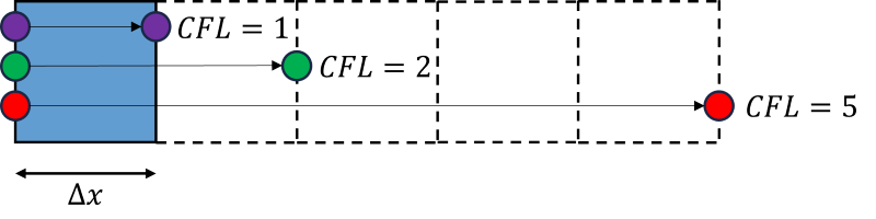
Now we insert a particle that is flowing with the local velocity [katex]u[/katex]. If we have a CFL number of 1, this means that the particle will exactly flow a distance of [katex]\Delta x[/katex], i.e. one cell width. If it is 2, then it will flow the distance of [katex]2\Delta x[/katex], i.e. 2 cell widths, and for a CFL number of 5, we get [katex]5\Delta x[/katex], i.e. 5 cell widths.
Let's look at the definition of the CFL number again (for convection-dominated flows, which is typically what we assume if we do not further specify which type of CFL number we are talking about):
\mathrm{CFL}=\frac{u\Delta t}{\Delta x}We said that for a CFL number of 1, a particle will flow exactly one cell width in space. The numerator is [katex]u\Delta t[/katex], which provides a length, and this has to be the same as [katex]\Delta x[/katex] for the CFL number to be 1. Since we said that we want to keep [katex]u[/katex] and [katex]\Delta x[/katex] constant, the only variable we can change is [katex]\Delta t[/katex] to match the CFL number we desire.
Thus, the CFL number is a local, non-dimensional time step based on the cell's size and velocity!
If we now assume that the cell size can vary in our mesh and that the local velocity will change from cell to cell (which is usually the case), then we can see that we can obtain widely different CFL numbers for each grid cell. In fact, for cases where we want to resolve turbulent boundary layers and we have a fine grid near the wall, say down to a [katex]y^+[/katex] value of 1, then we get very small cells in the boundary layer that are orders of magnitude smaller than the large cells in the farfield. By extension, the CFL number will vary by several orders of magnitude!
OK, so hopefully, this viewpoint makes sense. Whenever you see the CFL number now, think of it as a non-dimensional time step that restricts how far information (or particles) can propagate in one-time step. Let's now investigate why explicit and implicit schemes have different stability constraints.
Explicit time integration
In order to understand the von Neumann stability analysis intuitively, we need to look at the stencil of the different numerical schemes. A stencil is just a graphical representation of the numerical scheme you are using, and we plot the stencil in an [katex]i,n[/katex] plot, where the x-axis ([katex]i[/katex]) represents the cells (here, a 1D mesh) and the y-axis ([katex]n[/katex]) the time axis. Take, for example, the linear advection equation we looked at before. For a first-order upwind scheme, we had:
u^{n+1}_i=u^n_i-a\frac{\Delta t}{\Delta x}(u^n_i-u^n_{i-1})We can see that in order to compute [katex]u^{n+1}_i[/katex], we need [katex]u^n_i[/katex] and [katex]u^n_{i-1}[/katex]. We place points for each of these in the [katex]i,n[/katex] plot and then connect them through an arrow to the time level [katex]n+1[/katex], i.e. the time level at which we are seeking the solution. This is shown in the plot below:
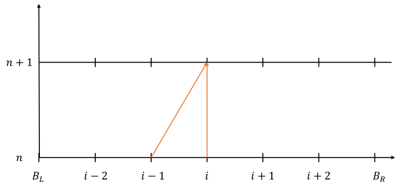
From this plot, we can see that [katex]u^{n+1}_i[/katex] depends on two cells from the previous time level. Now, let's bring back the CFL condition. For this equation, we obtained the result that the maximum allowable CFL number is 1. We also saw that the CFL number is just a non-dimensional time step, i.e. a CFL number of 1 means that information (or a particle) can only travel one cell width, i.e. from, say, [katex]i-1[/katex] to [katex]i[/katex]. In this case, this happens to be the same distance as the length of the stencil at time level [katex]n[/katex].
We see that in order to compute [katex]u^{n+1}_i[/katex], we only need (or rather, we only have) information available from the previous time step. Thus, if there is a disturbance in, say, cell [katex]i-2[/katex], we have no way of knowing that it exists. The stencil doesn't include that cell. If our CFL number increases to a value larger than 1, then a hypothetical particle (or, in general, some disturbance or pressure wave) could travel more than one cell's width. But our stencil would have no chance of capturing that!
This doesn't mean, though, that if we used a higher-order scheme, which will have a larger stencil, that your max allowable CFL number increases. It is still limited to one, which, unfortunately, isn't really intuitive.
There is a nice analogy that may help explain this, for which we need to review the Mach number. It is a measure of the local speed compared to the speed of sound, i.e. the fastest speed at which information (waves) can travel. It is defined as:
\mathrm{Ma}=\frac{u}{a}where [katex]u[/katex] is the local velocity and [katex]a[/katex] the local speed of sound. Let's say we are travelling with our private Harrier jet because we collected 7 million Pepsi points. After take-off, we fly with a velocity that is below the speed of sound, and so our Mach number is less than one. The flow is deemed subsonic, and this is shown in the image below on the bottom left.
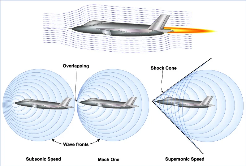
Here, we see how pressure waves will be travelling in all directions as they hit the nose of our aircraft. Pressure waves travel at the local speed of sound, and so they travel with a speed of [katex]a-u[/katex] to the left and with [katex]a+u[/katex] to the right.
We go over international waters and go pedal to the metal (aircraft do have acceleration and breaking pedals, right?). We hit Mach 1, i.e. the pressure waves are now travelling at the same speed as us, forming overlapping circles.
Information about our presence can no longer be propagated to air in front of the aircraft for it to move out of the way. If we fly subsonically, i.e. Mach less than one, the air in front is made aware of our presence and moves out of the way, as seen in the streamlines at the top of the figure.
Now, as we go up through the gears (a gearbox, seriously, Tom?) and activate nitro boost (please don't take my aeronautical engineering degree away from me ...), we hit Mach greater than one and go supersonic. Pressure waves can no longer keep up with us as our velocity has become greater than that of the local seed of sound, and thus [katex]a-u<0[/katex], i.e. the circles will have a negative velocity and start moving to the right, as seen in the figure above at the bottom right.
Here's a fancy description I once read in a book: "Taking the loci of all circles forms a shock front". Or, in plain English, draw a line that touches all circles at one point, and you get a shock front. Any air molecule to the left of that shock front has no way of knowing we are there.
Ok, great, what were we talking about again? Ah, yes, the CFL number. How does that relate? Well, let me write the CFL number slightly differently:
\mathrm{CFL}=a\frac{\Delta t}{\Delta x}=a\frac{1}{u}=\frac{a}{u}In other words, we are comparing the advective speed [katex]a[/katex] with some local speed [katex]u[/katex], i.e. a velocity ratio. Now [katex]a[/katex] in this example isn't the same as the local speed of sound seen above (poor choice of variable name, I know, I am following naming conventions here), but we can see some form of resemblance to the Mach number.
Now compare the stencil plot for the explicit first-order upwind discretisation with that of the Mach cone (which is formed by our aircraft in the figure above on the bottom right). We can see further similarities in a graphical sense.
If we have a CFL number of one, information travels as far as our stencil size (at least in one direction). Going beyond this will make the simulation unstable (i.e. divergence), as information or disturbances can now travel beyond our stencil, which has no way of capturing these disturbances.
Similarly, if we look back at the Mach cone in the figure above with our aircraft travelling at supersonic speeds, we could not detect any disturbance outside the Mach cone (to the left). We can fly faster beyond a Mach number of 1 (increasing the strength of the shock waves), but we can't change the speed of sound. In analogy, we can increase the time step beyond a CFL number of 1 (increasing the rate of divergence), but we can't change the information propagation speed inherent in our stencil.
I should stress that this is an analogy, and it probably breaks down if we look at Mach numbers above one. Here, the Mach cone simply reduces in size, but this isn't the case for the stencil (though the max allowable CFL number will likely be smaller than 1, but there is no dependence on the Mach number here).
Hopefully, though, this discussion helped a bit in realising that the CFL number simply limits the speed of information and that there is a natural limit to how far information can travel, similar to the local speed of sound.
Let's also look at the case of pure diffusion. As a reminder, the discretised equation using a central scheme for the spatial derivative and explicit time integration was given as:
u^{n+1}_i=u^n_i+\Gamma\frac{\Delta t}{(\Delta x)^2}(u^{n}_{i+1}-2u^{n}_i+u^{n}_{i-1})The corresponding stencil diagram is given below:
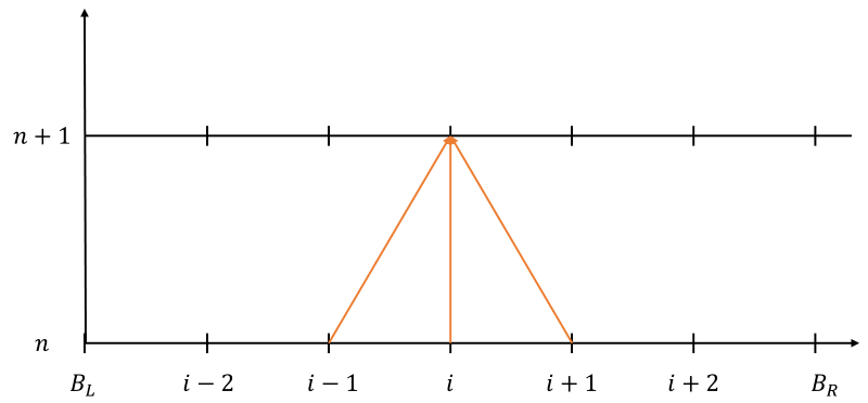
We see that we have the velocity at [katex]u^{n+1}_i[/katex] now depend on not just [katex]u^n_{i-1}[/katex] and [katex]u^n_i[/katex] but also [katex]u^n_{i+1}[/katex]. The stencil is symmetric, which we can see in the figure above.
Unlike the pure advection case, we saw that the max allowable (viscous) CFL number was 0.5 instead of 1. You may be thinking that this is half, but you would be wrong. To see why, let's look at a hypothetical particle again that travels within a cell. For the pure advection case, we said that a CFL number of 1 means that a particle is travelling across one cell width, i.e. [katex]\Delta x[/katex]. But pure advection also means that the direction of travel is in one direction only.
In the case of pure diffusion, a hypothetical particle can now travel both to the left and right. A CFL number of 0.5 means that this particle can now travel half a cell's width ([katex]\Delta x/2[/katex]) to the left or to the right, and the total distance is still one cell width ([katex]\Delta x[/katex]). It makes the max allowable time step smaller, but the information propagation speed is the same as for the linear advection case (now just in two opposing directions instead of one direction).
Makes sense? Hopefully! I think this was enough for the explicit time integration case. Now, let's see why implicit schemes are unconditionally stable!
Implicit time integration
We start again with the linear advection equation using a first-order upwind discretisation but now with an implicit time stepping. The equation was given before as:
u^{n+1}_i=u^n_i-a\frac{\Delta t}{\Delta x}(u^{n+1}_i-u^{n+1}_{i-1})Since we now have velocities that are evaluated at time level [katex]n+1[/katex], our corresponding stencil diagram looks as follows (ignore the dashed lines for now):
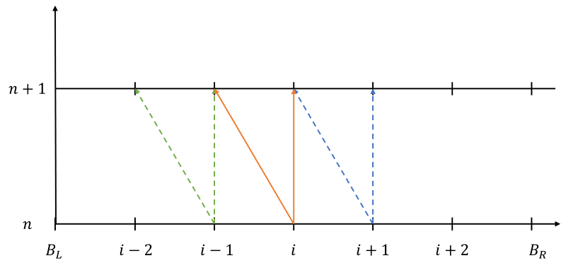
We saw before that evaluating the velocities at time level [katex]n+1[/katex] means that we cannot compute [katex]u^{n+1}_i[/katex] directly anymore and need to solve a linear system of equations. We see from the figure (and equation) above that in order to compute [katex]u^{n+1}_i[/katex], we need to know what [katex]u^{n+1}_{i-1}[/katex] is. So let's write the equation for that:
u^{n+1}_{i-1}=u^n_{i-1}-a\frac{\Delta t}{\Delta x}(u^{n+1}_{i-1}-u^{n+1}_{i-2})This equation is visualised by the green dashed line in the figure above. We see that this, in turn, depends on [katex]u^{n+1}_{i-2}[/katex]. Ok, so let's write out the equation for this as well:
u^{n+1}_{i-2}=u^n_{i-2}-a\frac{\Delta t}{\Delta x}(u^{n+1}_{i-2}-u_{B_L})We see that if we keep doing this, at some point, we will no longer have a dependence on the velocity to the left, as we are eventually hitting the boundary. In this case, instead of requiring the solution at [katex]u^{n+1}_{i-3}[/katex], we can replace that with the boundary conditions, i.e. [katex]u_{B_L}[/katex].
Compare that to the explicit time discretisation case. Here, the velocity at [katex]u^{n+1}_i[/katex] only depended on known quantities at the previous time level, i.e. [katex]n[/katex]. Each equation could be solved independently at node [katex]i[/katex], and a new velocity was obtained explicitly at time level [katex]n+1[/katex].
For implicit schemes, all equations are tightly coupled at time level [katex]n+1[/katex] and thus, the linear system of equations solves all of these equations at the same time. Thus, the effective computational stencil is as large as the computational domain. If we have any disturbances outside our local stencil, it doesn't really matter. All equations are coupled, and through the solution to the linear system, every cell will be able to know about the disturbance.
Thus, implicit schemes, through their tight coupling to one another, allow for an arbitrarily large CFL number.
This also explains why elliptic equations of the form
\nabla^2\phi=0
have to be solved implicitly. Elliptic equations, by nature, do not impose any speed restriction on how fast disturbances propagate, and a disturbance felt at one point in the flow would have to be felt anywhere else in the flow. This is the reason streamlines start to deviate before hitting an airfoil if we travel with a subsonic speed, as the elliptic behaviour of the pressure allows for air molecules to know about the presence of the airfoil before it has even arrived.
Thus, elliptic equations do not have a time derivative (which would allow for an explicit discretisation and thus a limit on how fast information can propagate). If you want to see how to discretise the above equation with an implicit discretisation and then how to solve it with a linear system solver, I've got you covered.
For completeness, let's also review the case of pure diffusion. The implicit version is given as:
u^{n+1}_i=u^n_i+\Gamma\frac{\Delta t}{(\Delta x)^2}(u^{n+1}_{i+1}-2u^{n+1}_i+u^{n+1}_{i-1})The corresponding stencil diagram is given as:
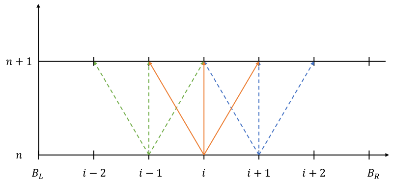
We now need to write equations for both [katex]u^{n+1}_{i+1}[/katex] and [katex]u^{n+1}_{i-1}[/katex] if we want to solve for [katex]u^{n+1}_i[/katex]. Thus, we need to formulate equations for both nodes accordingly, which is shown by the green and blue dashed stencils. These, in turn, will depend on their neighbouring velocities and eventually on the boundary values on the left and right, which are assumed to be known.
Hopefully, this discussion helped you understand the differences between explicit and implicit discretisation methods in a more schematic way. Now that we have all achieved black-belt status, let us look at some useful time-stepping techniques we can use to take control of our simulation and make it converge as fast as we wish!
Time-stepping techniques
With the knowledge we have gained thus far, we are able to determine a stable time step. If that is all we ever wanted to do, great, we could stop here and call it a day. However, the reality is that we have ever-increasing demands for larger and more complex simulations, but we don't really want to spend more time on our simulations. So, could we perhaps employ some clever time-stepping techniques to get faster convergence? We sure can, and in the following, I show you 4 popular techniques!
Adaptive time stepping
Adaptive time stepping is probably the simplest technique of them all. In this case, we say that instead of advancing our solution in time using a constant time step, we want to advance the solution at a constant CFL number to always integrate our solution in time with the highest time step possible. This will ensure that we reach convergence within the fewest steps possible.
Let's say you are simulating a flow where the velocity, on average, is decreasing over time. If we picked a constant time step (and assume that the grid size does not change), then our CFL number would, on average, decrease over time for each cell. Or, we could have a case where the average velocity is increasing over time. In this case, the CFL number will also increase and keeping the time step constant means we may end up with a CFL number that is above the max allowable one.
During the beginning of a simulation, it is rather normal that we have quite drastic changes in the velocity field. The initial conditions are typically far away from the final solution and do not satisfy the boundary conditions. In the first few iterations, this is corrected quickly, and this can lead to drastic changes, which become minute as we progress in time/iterations.
Therefore, we fix the CFL number at the beginning of the simulation and then use that to calculate a stable time step that gives us the fastest convergence (the fewest time steps overall to reach a specified simulated time). This can be written as
\Delta t_{max}=\max\left(\frac{\mathrm{CFL}\Delta x_i}{u_i}\right)\quad\forall i\in NHere, the index [katex]i[/katex] goes over all cells in the mesh, where we have [katex]N[/katex] cells. The above equation is fancy mathematics for the following implementation:
int main() {
  // setting up simulation, e.g. read parameters, read mesh, allocate memory for arrays
  // ...

  // loop over time
  while (currentTime < totalTime) {

    // calculate stable time step
    double dt = 0.0;
    double dtTemporary = 0.0;
    for (int i = 0; i < N; ++i) {
      dtTemporary = CFL * dx[i] / u[i];
      if (dtTemporary > dt) {
        dt = dtTemporary;
      }
    }

    // perform time step update, e.g. solve equations here
    // ...

    currentTime = currentTime + dt;
  }

  return 0;
}
Here, the variables dx and u are arrays that have the same length as the mesh and store the local mesh spacing and velocity for that cell. This is an implementation for a 1D case. If this is a 2D or 3D case, we have to replace dx[i] with the square root of the cell area or the cube root of the cell volume, respectively, while u[i] simply becomes the velocity magnitude, e.g. uMag = std::sqrt(std::pow(u[i], 2) + std::pow(v[i], 2) + std::pow(w[i], 2)). This is for 3D. If it is in 2D, we ignore the last component, i.e. std::pow(w[i], 2).
There is one problem with adaptive time stepping we need to be aware of. If our goal is to perform some frequency analysis on some signal in the flow, say, we want to investigate some vortex shedding, we need a constant time step size for our (fast) Fourier transform ((F)FT). If we use adaptive time stepping, then our time step will be anything but constant.
In this case, we have two options: Either we take the pain and use a constant time step, or we have to perform some interpolation on our signal. This would typically mean reading in the signal (i.e. two arrays, one for the current time and one for the signal itself, say the velocity component in the x direction), specifying a new time array with a constant time step at which we want to know the signal, and then using the already obtained signal to do some linear interpolation to obtain values for the signals at entries in the new time array.
Local time stepping
Local time stepping is the next logical step up from adaptive time stepping. While we used a constant time step size per time step in adaptive time stepping, local time stepping computes the maximum allowable time step size per cell for each iteration. This means that we no longer just have a single value for the time step size [katex]\Delta t[/katex], but instead an array where each cell in the mesh has its own time step [katex]\Delta t_i[/katex].
Let's look at an example where adaptive time stepping is breaking down. Say we have several orders of magnitude differences between the smallest and the largest cells. This is very common when we want to resolve the boundary layer with a fine resolution, say with a [katex]y^+[/katex] value of 1. The largest velocities are likely recorded near the boundary layer (especially if our geometry has curvatures that locally accelerate the flow, like the leading edge of an airfoil). Thus, using the definition for the time step size again:
\Delta t=\mathrm{CFL}\frac{\Delta x}{u}If the cells are small but the local velocity is high, the above equation tells us that the local time step size must be the smallest. Compare that to cells in the farfield where the cell sizes are orders of magnitude larger, while the velocity may be even smaller than near the boundary layer. Here, the max allowable time steps would be orders of magnitudes larger compared to the one obtained near the boundary layer.
For adaptive time stepping, we need to take the maximum allowable time step that is satisfied in all cells. This means that there is only really one cell in which we run at the maximum allowable CFL number, while all other cells use the same time step, although they could tolerate a larger time step size based on the CFL condition.
This is where local time stepping comes in. Now we say that each cell can march at its own time step size to accelerate convergence. Now, doing this will destroy any time accuracy, as we are no longer marching at the same time step, and so we can't do this for unsteady simulations. The only time local time stepping works is when we want to use time stepping to march to a steady state solution. For a steady state, there is no dependence on the time, by definition, and so we let each cell converge as quickly as they can to the steady state by using their optimal time step size.
This also shows the power of time stepping. Even if we are interested in a steady-state solution, we very often use an unsteady problem formulation for our simulation, only to be able to use some of the advanced time-stepping techniques that will accelerate convergence. Once a steady state is reached, the solution does not change in time anymore (by definition), and so any time derivative that appears in our governing equations will be zero. This type of time stepping is typically referred to as pseudo-time stepping.
Local time stepping is powerful in accelerating convergence, but if you want to crank it up to 11 and really get a stupidly fast convergence rate, then you need CFL ramping.
CFL ramping strategies
CFL ramping strategies are one of my favourite things in CFD. If they are implemented correctly and work well for the test case you are investigating, then they can really make your simulation converge almost as quickly as you like. Bücker et al. 2008 provide an excellent review of available CFL ramping strategies, of which we will review the switched evolution relaxation (SER) method.
The theory is as follows: At the beginning of the time stepping, we already established that changes in the velocity (and other) fields are rather large. But, once we have gone through this initial phase of adjusting our incorrect initial condition to the boundary conditions in our simulation, the simulation starts to converge towards the solution, but at a rather slow rate.
Thus, the idea behind SER (and other ramping strategies) is to increase the CFL number as the simulation converges. This, in theory, should accelerate convergence and provide faster solutions. The way SER works is by computing a CFL number now for each time step that is based on the change in residuals. We can pick any residual we like, say the residual of the density, if we are working with a compressible code.
The residual, in turn, is defined as the difference of a variable between two subsequent iterations/time steps. Sticking with the density as an example, we could compute the density residual for each cell [katex]i[/katex] at time step [katex]n[/katex]:
\mathrm{Res}(\rho)^{n}=\rho^{n}_i-\rho^{n-1}_iThis will give us a vector where we have a residual value for each cell. Taking the L2 vector norm of this residual vector will provide us with a single scalar value that is representative of the residual. The L2 norm is defined as:
\lVert \mathrm{Res}(\rho)\rVert_2=\sqrt{\sum_{i=0}^N \mathrm{Res}(\rho)_i^2}At the first iteration, we will compute a residual that is denoted by [katex]\lVert \mathrm{Res}(\rho)^0\rVert_2[/katex]. As we progress with our simulation and we are converging, we see that residuals are dropping and thus we would expect that [katex]\lVert \mathrm{Res}(\rho)^0\rVert_2>\mathrm{Res}(\rho)^n\rVert_2[/katex], i.e. the residuals at time level [katex]n[/katex] should be smaller than at the first iteration.
Next, we need to define a minimum and maximum allowable CFL number that we want to use. These two numbers will be used to ensure that our CFL number does not go out of this bound as we calculate an adaptive CFL number. Let's call them [katex]\mathrm{CFL}_{min}[/katex] and [katex]\mathrm{CFL}_{max}[/katex]. Then, we can compute the CFL number at time level [katex]n[/katex], using the SER method, as:
\mathrm{CFL}^n=\mathrm{CFL}_{min}\cdot\left(\frac{\lVert \mathrm{Res}(\rho)^0\rVert_2}{\lVert \mathrm{Res}(\rho)^n\rVert_2}\right)^\alphaSince the residuals at time level [katex]n[/katex] are expected to be below the residuals at the first iteration, we would expect the fraction to grow as we converge. We take that fraction to the power of [katex]\alpha[/katex], which allows us to increase this fraction slightly if we want to. This is then multiplied by the minimum CFL number, and thus, we can see that as the residuals are getting smaller and smaller, our CFL number, and by extension, the time step, will increase. If [katex]\mathrm{CFL}^n[/katex] is larger than [katex]\mathrm{CFL}_{max}[/katex], we simply use [katex]\mathrm{CFL}_{max}[/katex].
If you couple CFL number ramping like the SER method with local time stepping, magic happens. As your residuals drop, the CFL number increases, but because your CFL number increases, the residuals drop even faster. This is a positive feedback loop that drives down residuals very quickly.
Of course, using this method requires a fully implicit solver to begin with, so if you use a method like the SIMPLE or PISO algorithm (where the first two letters in SIMPLE stand for Semi-implicit (i.e. not fully implicit)), and you are not using a fully implicit version of it, then you won't be able to use SER. Sorry, OpenFOAM users. If you are using SU2, they use a fully implicit discretisation and have a working implementation of a CFL ramping strategy, which we discussed some time ago when we looked at SU2.
Applications for explicit and implicit time integration
Now that we have a good understanding of what implicit and explicit methods are, I wanted to look at typical application areas where explicit and implicit methods shine. Use these as a starting point if you develop your own solver and want to know if you need implicit methods or if explicit methods would do just fine as well.
When to use explicit time integration
Let's start simple. When you start writing your own solver, you want to start with an explicit time-stepping method. It is cheap and easy to implement, which makes it easy to debug. Your test cases will be simple and likely have a uniform grid anyway, so you are not getting any advantage of using an implicit method as your CFL number is likely close to 1 anyway. In my opinion, only once your solver matures and you are able to handle grids of varying cell sizes should you look into implicit methods.
This only works if the solver you are implementing supports a fully explicit discretisation. If it doesn't, well, then you have to take the pain and support the solution to a linear system of equations, i.e. [katex]\mathbf{Ax}=\mathbf{b}[/katex]. The SIMPLE algorithm is such an example that requires a linear system due to its semi-implicit nature. For incompressible flows, I would start with the artificial compressibility method, which allows for a fully explicit time integration. For compressible flows, the Euler equation can be solved explicitly just fine.
Let's say your solver is maturing, but you only plan to support the Euler equation for compressible flows. In this case, you drop the viscous terms in the Navier-Stokes equation and thus only retain the inviscid part. This is a reasonable approximation for high-speed flows, but you won't be able to resolve any boundary layer. This means that you no longer need a fine grid resolution near the boundary layer and thus have a more uniform mesh size throughout your grid. This, in turn, means that your local time step sizes will be closer together overall and explicit time stepping works well here.
If you are thinking of supporting Cartesian grids only, perhaps with some non-conformal mesh refinement of at most 1-2 levels, your local mesh sizes will also be comparable. But, once you increase the number of refinement levels, you increase the difference between the smallest and largest cells and get into similar issues as discussed previously, i.e. a large spread of max allowable time step size within each cell.
Finally, there is turbulence modelling. If you are interested in running scale-resolved simulations, such as Large-Eddy Simulations (LES) or Direct Numerical Simulations (DNS), then you likely do not only have to obey the CFL number but also other local time step size restrictions, as you want to resolve turbulence in time (which is the whole point of using LES and DNS compared to RANS, which is steady state by definition).
For a DNS, for example, you probably want to resolve, or at least closely capture, the Kolmogorov microscales, which state what the smallest length, time, and velocity scales are in your flow. The Kolmogorov microscale for time is defined as:
\tau=\sqrt{\frac{\nu}{\varepsilon}}Here, [katex]\nu[/katex] is the kinematic viscosity and [katex]\varepsilon[/katex] is the dissipation rate. If you compute this unit within each cell of your domain and then compare that to the time step size based on the CFL number, you will often find that [katex]\tau[/katex] will be smaller than [katex]\Delta t[/katex], and so you are naturally restricted in your time step size. No need for fancy implicit time-stepping, as you cannot go near a CFL number of 1 anyways.
For this reason, a lot of research codes that are used for LES and DNS computation prefer not just explicit time stepping but higher-order explicit time stepping schemes, such as the Runge-Kutta method.
When to use implicit time integration
Continuing from our discussion on explicit methods, you have written your code, it is working with explicit time stepping, at some point you may want to switch to implicit methods. When is the right time to switch? Well, you will know because running your code becomes painful, and you really feel that you want to increase your CFL number but find yourself unable to because of your explicit time discretisation.
Typically, this is the case when you start to look at more complex geometry (and there is naturally more variation in the cell sizes), or you deal with unstructured grids, or you are trying to resolve boundary layers with a fine grid size near the wall. These are all scenarios where you want to reconsider your time-stepping philosophy.
Another reason may be that you want to resolve a process that takes place over a large time scale. For example, I once was involved in a project where we wanted to develop a new type of rover that could be used on Mars. We were interested in the heat loss of that rover during the night. The person who involved me clearly had no idea about CFD, as he asked me to perform a simulation of the rover in near vacuum conditions for a few simulated days (say, 120 hours, i.e. 5 days) to get an idea of how the temperature on the rover's surface changed over time.
If I wanted to simulate that with an explicit time integration scheme, where the time step size may have been limited to, say, [katex]\Delta t =10^{-5}[/katex], that would require a total of about 40 billion time steps, on a mesh with about half a million of grid points (already very coarse). In the end, we settled for a single steady-state simulation to extract some heat exchange coefficients and use that to perform some analysis.
The academic who involved me in the project then submitted the proposal to the European Space Agency to apply for some funding. It was rejected (thankfully), but the quintessential academic that he was, he thought, "I have already written up this proposal, which is about 20 pages, and it even has some CFD results (which I constantly stressed were very preliminary (coarse grid, no grid dependency study and all that jazz), why not publish that in a journal?"
He submitted and got rejected again, this time with a note from the handling editor that large portions of the manuscript contained clear signs of plagiarism, and for that reason, the paper must be rejected. He got back to the editor, and Pinky swore he would heavily revise the manuscript, but that was the last of him I heard. Honestly, afterwards, he vanished from the surface of the earth. Someone should put up a missing person picture or at least inform interpol ...
Where was I? Right, implicit time stepping. We said that for scale-resolving turbulence modelling, i.e. LES and DNS (throw in detached eddy simulations DES and scale-adaptive simulations SAS if you like), explicit time stepping is pretty much all but inevitable. But for turbulent simulations involving RANS, potentially coupled with a pseudo time stepping approach, implicit methods are really useful and probably what you want to use.
This brings me to the main use of implicit methods: General-purpose CFD solvers. If you want to support a large user base without a specific application in mind, you need to go implicit. They may or may not enjoy the added ability to freely choose the CFL number. But more likely, they see CFD as a tool, one they have no interest in learning in detail but rather just use in their workflow, and they probably don't even know what explicit or implicit time stepping means, what the von Neumann stability analysis is, and what the CFL number is.
This is fine, not everyone wants or need to know, but if you want them to use your tool, you better make sure you have unconditional stability baked into your solver, otherwise they may run it with a time step that is too large and see their simulation crashing. They do that a few times until they decide you are an incompetent software developer and move on ...
Summary
And there we have it, another article that was planned to be about half the size, and somehow, I still managed to pack it with lots of ideas that popped up as I was writing the article.
I hope you now have a better understanding of the differences between explicit and implicit time stepping. The main difference is that explicit methods are always conditionally stable, at best, while implicit methods enjoy unconditional stability.
This means explicit methods are limited in the max allowable time step size they can use, which is typically limited to a CFL number of 1 for convection-dominant flows, i.e. one where the Reynolds number is much larger than 1 (if your flow is turbulent, it is convection-dominant). For viscous cases, the max allowable (viscous) CFL number reduces to 0.5 and is defined slightly differently.
We looked at the von Neumann stability analysis and how this can be applied to explicit and implicit methods for different numerical schemes. We looked at a generic way of deriving a stability condition and then plotted it in a complex plane to visually determine the maximum allowable CFL numbers. This approach will work for any other numerical scheme as well.
We also looked at a graphical representation of the CFL number and how we can develop some intuition where this max allowable CFL number of 1 comes from, as well as why implicit schemes do not have this limitation, and finally reviewed some time stepping techniques that are available to us to accelerate convergence.
Finally, we reviewed applications in which you may want to go for either explicit or implicit time-stepping techniques, and by now, you should have a good idea about when to use which scheme and how stable your scheme is going to be. In the next article, we will look at numerical schemes in more detail, including popular time-stepping schemes.
Acknowledgements
Special thanks to Alexander Schukmann for helping me to improve this article! Check out how you can contribute, too.
Tom-Robin Teschner is a senior lecturer in computational fluid dynamics and course director for the MSc in computational fluid dynamics and the MSc in aerospace computational engineering at Cranfield University.