What is numerical dissipation in CFD and why do we need it?
I'll make a bet with you. By the end of this article, you will have changed your views on numerical dissipation. When you read the words numerical dissipation in the title, did you associate that with something good or bad? My guess is that you view numerical dissipation as something bad, and that would be in line with the prevailing belief as far as I can see.
Numerical dissipation is a vital tool to stabilise our simulation, but we are not simply trading stability in favour of accuracy. We will see throughout this article that numerical dissipation is deeply rooted in physical phenomena. We will look at the origin of numerical dissipation and discuss how we can increase or reduce it. In the end, we look at how numerical dissipation really just resolves physical phenomena in both turbulence modelling and shock wave capturing methods, and we'll see numerical dissipation in action in a case study.
In this article
Introduction
If you read literature and reports on numerical dissipation in CFD simulations, you get the feeling that the majority of people would like to get rid of it. It is seen as something that contaminates the solution's accuracy, but nothing could be further from the truth. The reality is that we can't have a successful CFD simulation without at least some numerical dissipation; it is essential!
Numerical dissipation plays a crucial role in stabilising a CFD simulation. The stabilisation is rooted in physics and is not just a numerical artefact. We need numerical dissipation because we have removed physical dissipation elsewhere. And so, in this article, I want to look at the role of the often misunderstood numerical dissipation.
The key challenge in any CFD simulation is to balance the amount of numerical dissipation. We need some to stabilise the simulation but we want to control the amount so as to not excessively smooth our gradients. If the numerical dissipation went unchecked, we would risk loosing accuracy. Getting the amount right is a constant balancing act.
We will examine the relationship between numerical dissipation and turbulence modelling. We will see that all turbulence modelling removes physical dissipation, which we then need to match through numerical dissipation or other modelling strategies. In the extreme case, we simply take the numerical dissipation and assume it is proportional to the physical dissipation we removed.
Furthermore, if we want to solve compressible flows with strong gradients and shockwaves, numerical dissipation is vital to stabilise gradients near discontinuities. While shockwaves are, in reality, a smooth transition from one state to another, the scale at which this transition happens is so small that it is not resolved by CFD simulations (or, indeed, the governing equations). Thus, numerical dissipation is needed near shocks but should be removed elsewhere.
In this article, we will explore where numerical dissipation originates from, how we can control it, and then how we can leverage it for turbulent flows and shock-capturing applications. With that preamble out of the way, let's get started!
The origin of numerical dissipation
In this section, we will review where numerical dissipation originates from. We will first look at the modified equation analysis and see where numerical dissipation comes from. It serves as an introductory example, as all discretisation processes have similar properties. We then look at the role of the computational mesh, which itself introduces numerical dissipation.
The modified equation analysis
Whenever we are trying to obtain a solution for a governing equation in CFD, we have to do so by solving the equation numerically. The process of numerically solving an equation requires some form of discretisation. This requires the exact partial differential equation to be brought into an approximated algebraic form, which can be solved.
In the process, we no longer solve the original equation. Instead, the approximations we have done during the discretisation have slightly changed the governing equations, and the modified equation analysis is a tool we can use to visualise what equation we are solving.
We'll use the linear advection equation here to demonstrate how the modified equation analysis works. It would work the same way for more complex equations, but to keep things simple, let's go with it. The linear advection equation can be obtained by considering the Navier-Stokes equation and then assuming an incompressible flow with no diffusion and pressure gradients. To make it linear, the non-linear term needs to be linearised, which is achieved by replacing the velocity with a constant velocity [katex]a[/katex]. This equation is given as:
\frac{\partial u}{\partial t}+a\frac{\partial u}{\partial x}=0\tag{1}Now, there are as many different possibilities to discretise this equation into an algebraic form as there are VPN sponsorships on YouTube (this sentence will age badly, I assume!). Let's keep things simple and assume a simple first-order Euler time integration in time and a first-order upwind scheme in space. If we assume that [katex]a>0[/katex], then we can write the following discretised form:
\frac{u^{n+1}_i-u^n_i}{\Delta t}+a\frac{u^n_i-u^n_{i-1}}{\Delta x}=0\tag{2}Here, [katex]\Delta t[/katex] represents the time step we take to advance our equation in time, while [katex]\Delta x[/katex] represents the spacing on our mesh in space. If it is just a 1D mesh, as the equation suggests here, then it is simply the distance between the nodes on a discretised line.
Let's solve this equation for the only unknown, in this case, [katex]u_i^{n+1}[/katex]. This results in the following explicit formulation:
u^{n+1}_i=u^n_i-\frac{a\Delta t}{\Delta x}\left(u^n_i-u^n_{i-1}\right)\tag{3}This is the equation we want to solve, in the hope that we are getting a good approximation for our original governing equation, i.e. Eq.(1). But, choosing any other numerical discretisation would give us a different equation here. So, the modified equation analysis is trying to establish the contributions of each quantity that we don't know for certain.
Let's assume for the moment that [katex]u_i^n[/katex] represents the wind velocity at our location, indicated by [katex]i[/katex], and at the current time, indicated by the time level [katex]n[/katex]. We can measure the velocity and know its exact value. So, [katex]u_i^n[/katex] is known exactly.
Looking at Eq.(3), however, we also need to know the wind velocity at some other location [katex]i-1[/katex]. We don't have a way of measuring the velocity there, so we have to approximate it. This approximation will introduce an error. The same is true for the velocity in the future, i.e. [katex]u_i^{n+1}[/katex]. This value will be based on exact measurements, i.e. [katex]u_i^n[/katex] and some approximations [katex]u_{i-1}^n[/katex]. So, this value itself will be an approximation.
The modified equation analysis is telling us that we should check how well we are approximating these unknown values. To do so, we use a Taylor series, which provides us with an exact mechanism of determining quantities in the future or elsewhere in space. The only caveat: it has an infinite number of terms. Well, typically only the leading terms are important, while all higher-order terms can be dropped.
So let's develop these Taylor series for both [katex]u_i^{n+1}[/katex] and [katex]u_{i-1}^n[/katex]. For [katex]u_i^{n+1}[/katex], we get:
u^{n+1}_i=u^n_i + \frac{\partial u}{\partial t}\Delta t + \frac{\partial^2 u}{\partial t^2}\frac{(\Delta t)^2}{2!} + \frac{\partial^3 u}{\partial t^3}\frac{(\Delta t)^3}{3!} + \mathcal{O}[(\Delta t)^4]\tag{4}And, for [katex]u_{i-1}^n[/katex], we obtain:
u^{n}_{i-1}=u^n_i - \frac{\partial u}{\partial x}\Delta x + \frac{\partial^2 u}{\partial x^2}\frac{(\Delta x)^2}{2!} - \frac{\partial^3 u}{\partial x^3}\frac{(\Delta x)^3}{3!} + \mathcal{O}[(\Delta x)^4]\tag{5}Now we insert both Eq.(4) and Eq.(5) back into Eq.(3), acknowledging that the approximation we have done for both terms is fourth-order accurate in space and time, as indicated by the truncation term [katex]\mathcal{O}[/katex], i.e. the exponent of [katex]\Delta t[/katex] and [katex]\Delta x[/katex]. This results in:
u^n_i + \frac{\partial u}{\partial t}\Delta t + \frac{\partial^2 u}{\partial t^2}\frac{(\Delta t)^2}{2!} + \frac{\partial^3 u}{\partial t^3}\frac{(\Delta t)^3}{3!}=u^n_i-\frac{a\Delta t}{\Delta x}\left[u^n_i- \left(u^n_i - \frac{\partial u}{\partial x}\Delta x + \frac{\partial^2 u}{\partial x^2}\frac{(\Delta x)^2}{2!} - \frac{\partial^3 u}{\partial x^3}\frac{(\Delta x)^3}{3!}\right)\right]\tag{6}We have replaced here [katex]u^{n+1}_i[/katex] on the left-hand side of the equation, as well as [katex]u_{i-1}^n[/katex] within the parenthesis on the right-hand side. We can now simplify the equation. This involves getting rid of the [katex]u_i^n[/katex] on both sides as they cancel each other out, as well as factoring out [katex]\Delta t[/katex] on the left-hand side and [katex]\Delta x[/katex] on the right-hand side. We are left with:
\left(\frac{\partial u}{\partial t} + \frac{\partial^2 u}{\partial t^2}\frac{\Delta t}{2!} + \frac{\partial^3 u}{\partial t^3}\frac{(\Delta t)^2}{3!}\right)\Delta t=-\frac{a\Delta t}{\Delta x}\left(\frac{\partial u}{\partial x} - \frac{\partial^2 u}{\partial x^2}\frac{\Delta x}{2!} + \frac{\partial^3 u}{\partial x^3}\frac{(\Delta x)^2}{3!}\right)\Delta x\tag{7}If we divide both sides by [katex]\Delta t[/katex], and note that the right-handside contains [katex]\Delta x/\Delta x[/katex], we can further simplify the equation to:
\frac{\partial u}{\partial t} + \frac{\partial^2 u}{\partial t^2}\frac{\Delta t}{2!} + \frac{\partial^3 u}{\partial t^3}\frac{(\Delta t)^2}{3!}=-a\left(\frac{\partial u}{\partial x} - \frac{\partial^2 u}{\partial x^2}\frac{\Delta x}{2!} + \frac{\partial^3 u}{\partial x^3}\frac{(\Delta x)^2}{3!}\right)\tag{8}Now we solve the equation for [katex]\partial u/\partial t[/katex] so that it remains the only term on the left-hand side. We collect all other terms on the right-hand side, which produces:
\frac{\partial u}{\partial t} =-a\frac{\partial u}{\partial x} - \frac{\partial^2 u}{\partial t^2}\frac{\Delta t}{2} + a\frac{\partial^2 u}{\partial x^2}\frac{\Delta x}{2} - \frac{\partial^3 u}{\partial t^3}\frac{(\Delta t)^2}{6} - a\frac{\partial^3 u}{\partial x^3}\frac{(\Delta x)^2}{6}\tag{9}
At this point, comparing Eq.(9) to Eq.(1), we can see that the left-hand side of the equation combined with the first term on the right-hand side is again the original equation we started with. However, we have introduced a series of higher-order derivatives in both space and time on the right-hand side, which we will later see as our numerical dissipation.
If we think about dissipation in general, it is usually a process driven by second-order partial derivatives in space. However, Eq.(9) also contains derivatives in time, which we have to eliminate. We aim to express all time derivatives in equivalent spatial derivatives to see how strong our numerical dissipation will be. To do so, we must find an equivalent Taylor series for these time derivatives.
The first term we see in Eq.(9) that we want to get rid of is [katex]\partial^2 u/\partial t^2[/katex]. To do so, we simply take the time derivative of Eq.(9). Remember, the Taylor series approximation is exact (if all higher-order terms are considered), so taking the time derivative of it will still give us an exact relation for the second-order time derivative. Doing so will result in:
\frac{\partial^2 u}{\partial t^2} =-a\frac{\partial^2 u}{\partial x\partial t} - \frac{\partial^3 u}{\partial t^3}\frac{\Delta t}{2} + a\frac{\partial^3 u}{\partial x^2\partial t}\frac{\Delta x}{2} - \frac{\partial^4 u}{\partial t^4}\frac{(\Delta t)^2}{6} - a\frac{\partial^4 u}{\partial x^3\partial t}\frac{(\Delta x)^2}{6}\tag{10}This equation now contains mixed derivatives of the form [katex]\partial^{m}u/(\partial x^{m-1}\partial t)[/katex]. Not a problem, we can just abuse Eq.(9) again, and take the derivative of it with respect to [katex]x[/katex]. This results in:
\frac{\partial^2 u}{\partial x\partial t} =-a\frac{\partial^2 u}{\partial x^2} - \frac{\partial^3 u}{\partial x\partial t^2}\frac{\Delta t}{2} + a\frac{\partial^3 u}{\partial x^3}\frac{\Delta x}{2} - \frac{\partial^4 u}{\partial x\partial t^3}\frac{(\Delta t)^2}{6} - a\frac{\partial^4 u}{\partial x^4}\frac{(\Delta x)^2}{6}\tag{11}Multiplying Eq.(11) by [katex]-a[/katex] results in:
-a\frac{\partial^2 u}{\partial x\partial t} =a^2\frac{\partial^2 u}{\partial x^2} + a\frac{\partial^3 u}{\partial x\partial t^2}\frac{\Delta t}{2} - a^2\frac{\partial^3 u}{\partial x^3}\frac{\Delta x}{2} + a \frac{\partial^4 u}{\partial x\partial t^3}\frac{(\Delta t)^2}{6} + a^2\frac{\partial^4 u}{\partial x^4}\frac{(\Delta x)^2}{6}\tag{12}We can now add Eq.(10) and Eq.(12) togehter. We will see in a second why this is beneficial. Doing so will give us the following equation:
\frac{\partial^2 u}{\partial t^2} -a\frac{\partial^2 u}{\partial x\partial t} =-a\frac{\partial^2 u}{\partial x\partial t} + a^2\frac{\partial^2 u}{\partial x^2} - \frac{\partial^3 u}{\partial t^3}\frac{\Delta t}{2} + a\frac{\partial^3 u}{\partial x\partial t^2}\frac{\Delta t}{2} + a\frac{\partial^3 u}{\partial x^2\partial t}\frac{\Delta x}{2} - a^2\frac{\partial^3 u}{\partial x^3}\frac{\Delta x}{2} - \frac{\partial^4 u}{\partial t^4}\frac{(\Delta t)^2}{6} + a \frac{\partial^4 u}{\partial x\partial t^3}\frac{(\Delta t)^2}{6} - \\
a\frac{\partial^4 u}{\partial x^3\partial t}\frac{(\Delta x)^2}{6} + a^2\frac{\partial^4 u}{\partial x^4}\frac{(\Delta x)^2}{6}\tag{13}
This equation can be simplified by factoring out [katex]\Delta t/2[/katex] and [katex]\Delta x/2[/katex]. We can also see that we have [katex]-a\partial^2 u/(\partial x\partial t)[/katex] on both sides, so we can remove it from the equation. This gives us a much more digestible format of:
\frac{\partial^2 u}{\partial t^2} = a^2\frac{\partial^2 u}{\partial x^2} + \frac{\Delta t}{2}\left(a\frac{\partial^3 u}{\partial x\partial t^2} -\frac{\partial^3 u}{\partial t^3}\right) + \frac{\Delta x}{2}\left(a\frac{\partial^3 u}{\partial x^2\partial t} - a^2\frac{\partial^3 u}{\partial x^3}\right)+\mathcal{O}\left[(\Delta t)^2, (\Delta x)^2\right] \tag{14}This provides us with a second-order approximation for [katex]\partial^2/\partial t^2[/katex]. It still contains some mixed derivatives and time dependencies, and we will address that in a second. But for now, let's return to Eq.(9). In it, we saw that we also have to deal with third-order time derivatives. We use Eq.(10) again and derive it with respect to [katex]t[/katex]. This results in the following equation:
\frac{\partial^3 u}{\partial t^3} =-a\frac{\partial^3 u}{\partial x\partial t^2} - \frac{\partial^4 u}{\partial t^4}\frac{\Delta t}{2} + a\frac{\partial^4 u}{\partial x^2\partial t^2}\frac{\Delta x}{2} + \mathcal{O}\left[(\Delta t)^2,(\Delta x)^2\right] \tag{15}Now, you will have noticed that I was a bit cheeky here. I simply ignored the last two terms in Eq.(10). I did so because including them would have given me a third-order accurate prediction for my time derivative. However, I only know the second derivative with respect to time, i.e. Eq.(14), to second-order accuracy, so there is no point in dragging over higher-order derivatives in this case. Both Eq.(14) and Eq.(15) have the same order of accuracy.
Eq.(15) now contains a mixed derivate of the form [katex]\partial^3 u/(\partial x\partial t)[/katex]. We can find an equation for that by taking the derivative of Eq.(14) with respect to [katex]x[/katex]. This provides us:
\frac{\partial^3 u}{\partial x\partial t^2} = a^2\frac{\partial^3 u}{\partial x^3} + \frac{\Delta t}{2}\left(a\frac{\partial^4 u}{\partial x^2\partial t^2} -\frac{\partial^4 u}{\partial x \partial t^3}\right) + \frac{\Delta x}{2}\left(a\frac{\partial^4 u}{\partial x^3\partial t} - a^2\frac{\partial^4 u}{\partial x^4}\right) \tag{16}We will multiply this equation by [katex]-a[/katex] again, which produces:
-a\frac{\partial^3 u}{\partial x\partial t^2} = -a^3\frac{\partial^3 u}{\partial x^3} + \frac{\Delta t}{2}\left(-a^2\frac{\partial^4 u}{\partial x^2\partial t^2} +a\frac{\partial^4 u}{\partial x \partial t^3}\right) + \frac{\Delta x}{2}\left(-a^2\frac{\partial^4 u}{\partial x^3\partial t} + a^3\frac{\partial^4 u}{\partial x^4}\right) \tag{17}We can now add Eq.(15) and Eq.(17) together, which results in:
-a\frac{\partial^3 u}{\partial x\partial t^2} + \frac{\partial^3 u}{\partial t^3}= -a^3\frac{\partial^3 u}{\partial x^3} - a\frac{\partial^3 u}{\partial x\partial t^2} + \frac{\Delta t}{2}\left(-a^2\frac{\partial^4 u}{\partial x^2\partial t^2} +a\frac{\partial^4 u}{\partial x \partial t^3}\right) - \frac{\partial^4 u}{\partial t^4}\frac{\Delta t}{2} + \\
\frac{\Delta x}{2}\left(-a^2\frac{\partial^4 u}{\partial x^3\partial t} + a^3\frac{\partial^4 u}{\partial x^4}\right) + a\frac{\partial^4 u}{\partial x^2\partial t^2}\frac{\Delta x}{2} \tag{18}
Similar to what we saw in Eq.(13), the mixed derivative appears on both sides with the same coefficient and sign (since we multiplied by [katex]-a[/katex]), and so it will cancel out. We can also include the additional terms that contain [katex]\Delta t[/katex] and [katex]\Delta x[/katex] within the parenthesis. This exercise produces the following equation:
\frac{\partial^3 u}{\partial t^3}= -a^3\frac{\partial^3 u}{\partial x^3} + \frac{\Delta t}{2}\left(-a^2\frac{\partial^4 u}{\partial x^2\partial t^2} +a\frac{\partial^4 u}{\partial x \partial t^3} - \frac{\partial^4 u}{\partial t^4}\right) + \frac{\Delta x}{2}\left(-a^2\frac{\partial^4 u}{\partial x^3\partial t} + a^3\frac{\partial^4 u}{\partial x^4} + a\frac{\partial^4 u}{\partial x^2\partial t^2}\right) \tag{19}Now we have to make a decision. We have additional mixed derivative terms, and we could obtain additional equations for these as well. However, we would just end up adding more and more higher-order mixed derivatives. Therefore, we say that we are happy to take a first-order approximation of Eq.(19), which results in:
\frac{\partial^3 u}{\partial t^3}= -a^3\frac{\partial^3 u}{\partial x^3} + \mathcal{O}\left[\left(\Delta x\right), \left(\Delta t\right)\right] \tag{20}In a similar manner, we also take a first-order approximation of Eq.(16), which results in:
\frac{\partial^3 u}{\partial x\partial t^2} = a^2\frac{\partial^3 u}{\partial x^3} + \mathcal{O}\left[\left(\Delta x\right), \left(\Delta t\right)\right] \tag{21}We also need to have an equation for [katex]\partial^3 u/(\partial x^2\partial t)[/katex], as we can see in Eq.(10). To obtain this, we take the derivative with respect to [katex]x[/katex] twice in Eq.(9).
\frac{\partial^3 u}{\partial x^2\partial t} =-a\frac{\partial^3 u}{\partial x^3} - \frac{\partial^4 u}{\partial x^2\partial t^2}\frac{\Delta t}{2} + a\frac{\partial^4 u}{\partial x^4}\frac{\Delta x}{2} + \mathcal{O}\left[\left(\Delta x\right)^2, \left(\Delta t\right)^2\right] \tag{22}A first-order accurate expression is obtained by dropping the second and third terms on the right-hand side. This provides us with
\frac{\partial^3 u}{\partial x^2\partial t} =-a\frac{\partial^3 u}{\partial x^3} + \mathcal{O}\left[\left(\Delta x\right), \left(\Delta t\right)\right] \tag{23}We now insert Eq.(20), Eq.(21), and Eq.(23) back into Eq.(14). This provides us with a second-order time derivative that is now only dependent on spatial derivatives. The equation is as follows:
\frac{\partial^2 u}{\partial t^2} = a^2\frac{\partial^2 u}{\partial x^2} + \frac{\Delta t}{2}\left(a^3\frac{\partial^3 u}{\partial x^3} +a^3\frac{\partial^3 u}{\partial x^3}\right) + \frac{\Delta x}{2}\left(-a^2\frac{\partial^3 u}{\partial x^3} - a^2\frac{\partial^3 u}{\partial x^3}\right) \tag{24}Since both terms within both parentheses are equivalent, we can multiply one of them by two and remove the second term. This results in:
\frac{\partial^2 u}{\partial t^2} = a^2\frac{\partial^2 u}{\partial x^2} + \frac{\Delta t}{2}\left(2a^3\frac{\partial^3 u}{\partial x^3} \right) + \frac{\Delta x}{2}\left(-2a^2\frac{\partial^3 u}{\partial x^3}\right) \tag{25}Since the factor in front of the parenthesis contains [katex]1/2[/katex], this simplifies to:
\frac{\partial^2 u}{\partial t^2} = a^2\frac{\partial^2 u}{\partial x^2} + \left(a^3\Delta t-a^2\Delta x\right)\frac{\partial^3 u}{\partial x^3} \tag{26}With this equation in hand, we are now finally ready to express all time derivatives in Eq.(9) with spatial derivatives. To do that, we insert Eq.(20) and Eq.(26) back into Eq.(9). This produces the following equation:
\frac{\partial u}{\partial t} =-a\frac{\partial u}{\partial x} - a^2\frac{\partial^2 u}{\partial x^2}\frac{\Delta t}{2} - \left(a^3\Delta t-a^2\Delta x\right)\frac{\partial^3 u}{\partial x^3}\frac{\Delta t}{2} + a\frac{\partial^2 u}{\partial x^2}\frac{\Delta x}{2} + a^3\frac{\partial^3 u}{\partial x^3}\frac{(\Delta t)^2}{6} - a\frac{\partial^3 u}{\partial x^3}\frac{(\Delta x)^2}{6}\tag{27}We can now group derivatives together and factor out their coefficients. This produces the following:
\frac{\partial u}{\partial t} = -a\frac{\partial u}{\partial x} + \left(\frac{a\Delta x}{2}-\frac{a^2\Delta t}{2}\right)\frac{\partial^2 u}{\partial x^2} + \left(-\frac{a^3(\Delta t)^2}{2}+\frac{a^2\Delta x\Delta t}{2}+\frac{a^3(\Delta t)^2}{6}-\frac{a(\Delta x)^2}{6}\right)\frac{\partial^3 u}{\partial x^3}
\tag{28}
We can further clean up the equation by taking the factor [katex]a\Delta x/2[/katex] out for the second-order derivative, as well as the factor [katex]a(\Delta x)^2/2[/katex] for the third-order derivative. This results in the following:
\frac{\partial u}{\partial t} = -a\frac{\partial u}{\partial x} + \frac{a\Delta x}{2}\left(1-\frac{a\Delta t}{\Delta x}\right)\frac{\partial^2 u}{\partial x^2} + \frac{a(\Delta x)^2}{6}\left(-2\frac{a^2(\Delta t)^2}{(\Delta x)^2}+3\frac{a\Delta t}{\Delta x}-1\right)\frac{\partial^3 u}{\partial x^3} \tag{29}At this point, we can introduce the definition for the CFL number as:
CFL=\frac{a\Delta t}{\Delta x}\tag{30}If we introduce this definition of the CFL number back into Eq.(29), then we can further simplify the equation to:
\frac{\partial u}{\partial t} = -a\frac{\partial u}{\partial x} + \frac{a\Delta x}{2}\left(1-CFL\right)\frac{\partial^2 u}{\partial x^2} + \frac{a(\Delta x)^2}{6}\left(-2(CFL)^2+3CFL-1\right)\frac{\partial^3 u}{\partial x^3} \tag{31}At this point, we ignore the third-order derivative. By dropping this term, we end up with the following modified equation:
\frac{\partial u}{\partial t} = -a\frac{\partial u}{\partial x} + \frac{a\Delta x}{2}\left(1-CFL\right)\frac{\partial^2 u}{\partial x^2} + \mathcal{O}\left[(\Delta x)^2\right]\tag{32}If we bring the first term on the right-hand side onto the left-hand side, we recover the original equation plus an additional second-order derivative term on the right-hand side.
\frac{\partial u}{\partial t}+a\frac{\partial u}{\partial x}=\frac{a\Delta x}{2}\left(1-CFL\right)\frac{\partial ^2 u}{\partial x^2}\tag{33}Compare that with the one-dimensional momentum equation of the Navier-Stokes equation.
\frac{\partial u}{\partial t}+u\frac{\partial u}{\partial x}=-\frac{1}{\rho}\frac{\partial p}{\partial x}+\nu\frac{\partial ^2 u}{\partial x^2}\tag{34}Ignoring the pressure derivative, we see by direct comparison that we have the following relation:
\nu=\frac{a\Delta x}{2}\left(1-CFL\right)\tag{35}Thus, the modified equation analysis shows that the act of numerically discretising our equation leads to an additional term that has the appearance of diffusion. The coefficient of this second order derivative is known as the artificial viscosity, as it behaves just like viscosity but it is only there due to the numerical discretisation process.
Thus, this term is responsible for introducing additional diffusion, which we can also label as dissipation. Therefore, the artificial viscosity will introduce numerical dissipation. Both the artificial viscosity and numerical dissipation concept refer the essentially the same process.
Of course, we assumed here a simple finite difference, first-order upwind discretisation for our numerical scheme. But, if you were to do that for other schemes as well, you would find similar results.
In this case, we saw that we obtained both a second-order and third-order derivative in Eq.(31) through our modified equation analysis. For upwind-based schemes, the second-order derivative will dominate, while for others, it may be the third-order derivative.
As we have discussed, the second-order term mimics the physical process of dissipation, and the third-order term introduces a phenomenon known as dispersion. This introduces oscillations near discontinuities, and both numerical dissipation and dispersion are the two fundamental building blocks you will encounter when working with numerical schemes.
If we look again at our artificial viscosity parameter in Eq.(35), we see a clear dependence on the CFL number. Thus, it stands to reason that if our CFL number is 1, the artificial viscosity ought to be zero. So, let's see if the theory holds true.
Below is a simple step function that we wish to transport with our advection equation. We are using the same discretisation that was used for the modified equation analysis (i.e. first-order upwind in space and first-order Euler in time).
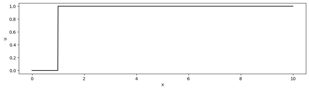
We have a step around [katex]x=1[/katex], and we can consider this a simple test case for how shock waves behave when approximated with a first-order numerical scheme. Using different CFL numbers in the time-stepping process, the following solutions are obtained when the discontinuity ought to be at [katex]x=5[/katex]:

Indeed, a CFL number of one (purple curve) results in no additional diffusion of the discontinuity. However, with a decreasing CFL number, the sharp interface is dissipated further into a smooth transition. This checks out as the artificial viscosity increases with a decreasing CFL number. Our theory is indeed confirmed.
Thus, the modified equation analysis demonstrates that upwind-based schemes introduce numerical dissipation through an additional diffusive term. We don't see the term in the discretised equation, but we can make it visible through the modified equation analysis.
The numerical scheme is not, however, the only source that introduces numerical dissipation. The computational grid plays just as much of an importance, and we will look at that next.
Grid resolution
As alluded to above, the computational grid is responsible for some numerical dissipation as well. For this consider the Figure below.
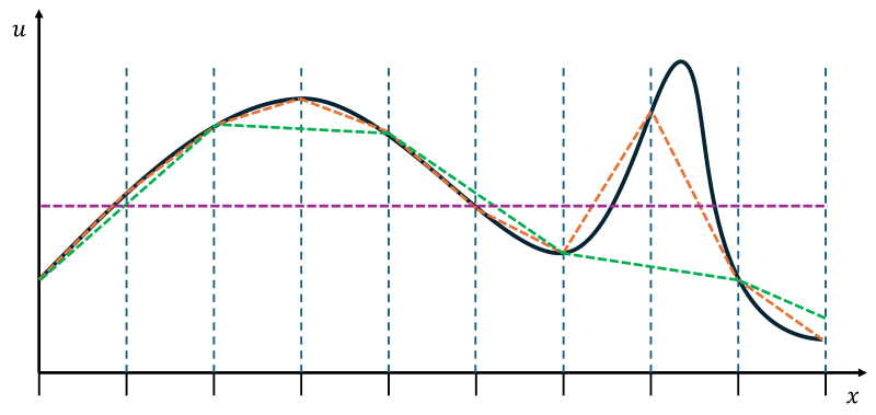
We have some analytic function of [katex]u[/katex] (black solid line) that we want to approximate. The blue dashed lines show the grid that we have along the [katex]x[/katex] axis. If we approximate this function on our grid, then the best resolution we are going to get is shown by the dashed orange line. It provides a fairly good approximation on the left side of the Figure, but it struggles to capture the sharp gradient on the right-hand side accurately.
Now consider the dashed green line. This line is obtained by omitting every second grid point, i.e. we have just made our grid coarser. It still does provide a reasonable approximation on the left, but we have no chance of capturing the sharp gradient on the right. As far as the coarse grid is concerned, there is no sharp gradient.
Now, imagine we only have a single grid point to approximate this function. We would simply get a flat line, which is indicated by the purple line. We could also say we are taking an average of the function at this point.
Now, let's investigate the diffusive term in the Navier-Stokes equation again. The diffusive term in the momentum equation is given as
\nu\frac{\partial^2 \mathbf{u}}{\partial \mathbf{x}^2} \tag{36}However, there are also diffusive terms in the energy equation (heat diffusion) and turbulent transport equation (e.g. diffusion of turbulent kinetic energy or dissipation). We saw in Eq.(33) and Eq.(35) that the artificial viscosity is also attached to a second-order derivative.
Diffusion acts against gradients and tries to equalise them. Consider the case of two metals at different temperatures. If we bring them into contact, their temperatures will, over time, equalise. We can calculate their new equalised temperature using a volume-averaged approach. If they have the same volume, then we simply take the average of the two temperatures. This is essentially what the Zeroth law of thermodynamics tells us.
Insert a tea bag into still water that has been boiled to 100 degrees. If we are careful enough and don't introduce any motion, then we'll see diffusion at play. Since there is no convection, the only process working on extracting the tea content with the water is diffusion. Again, we are trying to equalise gradients. In this case, we are equalising the concentration of tea, i.e. there is 100% in the tea bag and 0% in the water. We want the tea to be everywhere, and diffusion is helping us to do that.
If you are patient enough and had a way to measure tea concentration at different locations, you would see that eventually we would get tea everywhere, without any convective currents. Diffusion is slow, but over time, it will equalise gradients (e.g. in our two examples, temperature and tea concentration gradients).
Now go back to our figure above, we said that by creating a coarser grid, we take the average of the flow in the extreme case of having just a single grid point. But even if we have more than just one grid point, we saw that coarsening our grid results in a steady decrease in resolution. We saw how the resolution approached that of the average (just a single grid point), and so an under-resolved grid introduces numerical dissipation as well.
To add insult to injury, even if we have a fine grid, we can't win. We still get numerical diffusion if our cells are misaligned with the flow. We will look at this phenomenon next.
Grid and flow misalignment
So, the grid alignment also introduces numerical diffusion. How is that even possible? Well, we need to dig a bit deeper for this. We use an illustrative example again to help us see how this works. For this, we consider the following two cases:
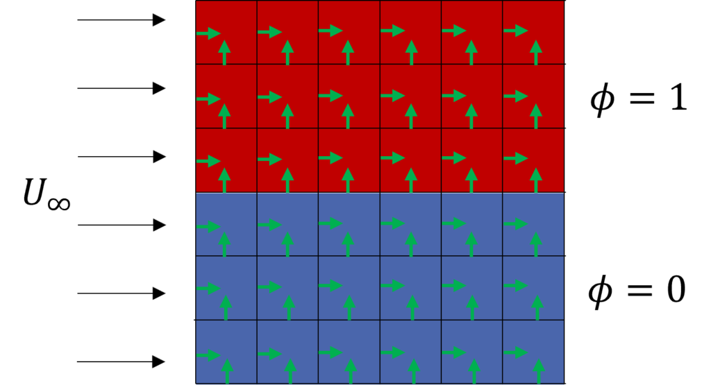
On the left, we have a square domain with structured cells where some flow is coming in on the left side of the domain. It does go through the domain and then leaves on the right. The top and bottom are symmetry boundary conditions, so that we don't introduce any unnecessary boundary layer.
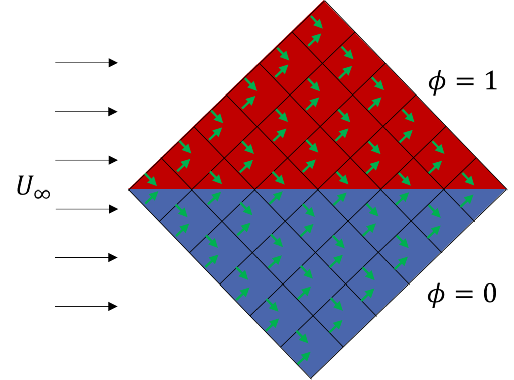
The second case on the right solves the exact same case and setup, with the only change being that the domain is turned by 45 degrees. This changes the orientation of the cells, where the normal vectors of each face, shown in green, are now at a 45-degree angle with the incoming flow. The first case has either a parallel or perpendicular alignment between its normal vectors and the incoming flow.
In both cases, we have added a passive scalar [katex]\phi[/katex]. If this is the first time you are hearing about a passive scalar, think of it as a quantity that is released into the flow to visualise its movement. The passive scalar is simply advected and diffused with the flow to visualise it.
The following video is a good demonstration of a passive scalar. Here, smoke is injected into a wind tunnel to visualise how flow is going around a car. The smoke follows the main flow but it does not influence it. Hence the name passive scalar.
The transport equation of a passive scalar is as follows:
\frac{\partial\phi}{\partial t}+u\frac{\partial\phi}{\partial x}=\Gamma\frac{\partial^2}{\partial x^2}\tag{37}We can see that it has a time derivative, so it can visualise changes in time (e.g. turbulent flow structures), it is being advected with the main flow's velocity [katex]u[/katex], and it has the capacity to diffuse with the flow, having a diffusion strength of [katex]\Gamma[/katex].
Now let's focus on the advection term [katex]u(\partial \phi/\partial x)[/katex], and bring that into context with our two cases we want to simulate above. In a finite volume discretisation, we have to discretise this term by taking a volume integral over each cell. This can be written as
\int_V u\frac{\partial \phi}{\partial x}\mathrm{d}V \tag{38}This integral is then transformed into a surface integral. We use the Gauss theorem (also called the divergence theorem) for that. This removes the derivative, and we now have to consider each facet of the cell (4 faces per cell for the quad cells we are considering in the two cases above), which introduces the normal vector of the face. This results in:
\int_A (u\cdot n\phi)_{f}\,\mathrm{d}A \tag{39}The surface integral has better conservation properties than the volume integral, and thus, we prefer this version of the integral over the volume integral. The last step in our approximation is to transform the volume integral into a summation. This requires us to only evaluate the surface integral at one discrete point on the face instead of considering how the flow changes over the entire face. In a sense, this is an averaging procedure. This results in:
\sum_{f=0}^{nFaces} u_f \cdot n_f \phi_f A_f \tag{40}We see that [katex]\phi_f[/katex] is now evaluated at the cell's faces (as indicated by the subscript). So, we need to find its value on the face. For this, consider the following case:
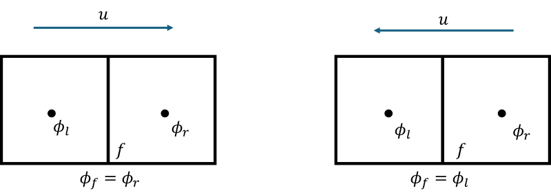
Here, we have two cells and want to obtain the value of [katex]\phi[/katex] at the face. For the case on the left, the velocity is going from the left to the right, and for the case on the right, it is going in the opposite direction, as indicated by the arrows above each case.
The naive approach would be to take a weighted average of its neighbouring values, i.e.
\phi_f=\frac{\phi_l+\phi_r}{2}\tag{41}However, this is a bad choice, and this scheme is unstable, leading to strong numerical oscillations in the solution. The oscillation occurs because we are not taking the direction of the flow into account. This has led to a flurry of new numerical schemes being developed that all take the direction of the flow into account.
One of them is the upwind scheme, which simply checks the direction of the flow and then sets the value at the face according to the following rule:
\phi_f=\begin{cases}\phi_l\quad u\ge 0\\\phi_r\quad u< 0\end{cases}\tag{42}The first case is what we see above on the left, i.e. the flow is positive, going from the left to the right, and so we set [katex]\phi_f=\phi_r[/katex]. In an upwind scheme, we set the value at the face based on the opposite direction of the flow (which is known as the upwind direction). So, if the flow is going from the left to the right, then we set the value at the face to whichever quantity is to its right. In this case, [katex]\phi_r[/katex]. This value goes from the right to the left to arrive from its cell centroid position at the face.
But now, consider the following case:
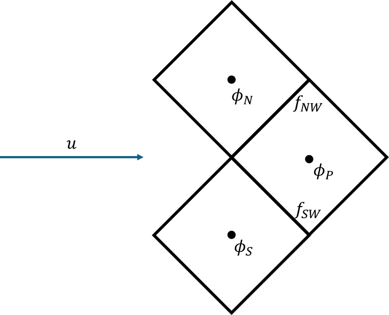
This was the second domain we considered above. The flow is still coming from the left and going to the right. But now, let's consider what happens at the interface of [katex]\phi[/katex], i.e. where its values change from 0 to 1, as we saw in the figure above. These are the two cases we may encounter:
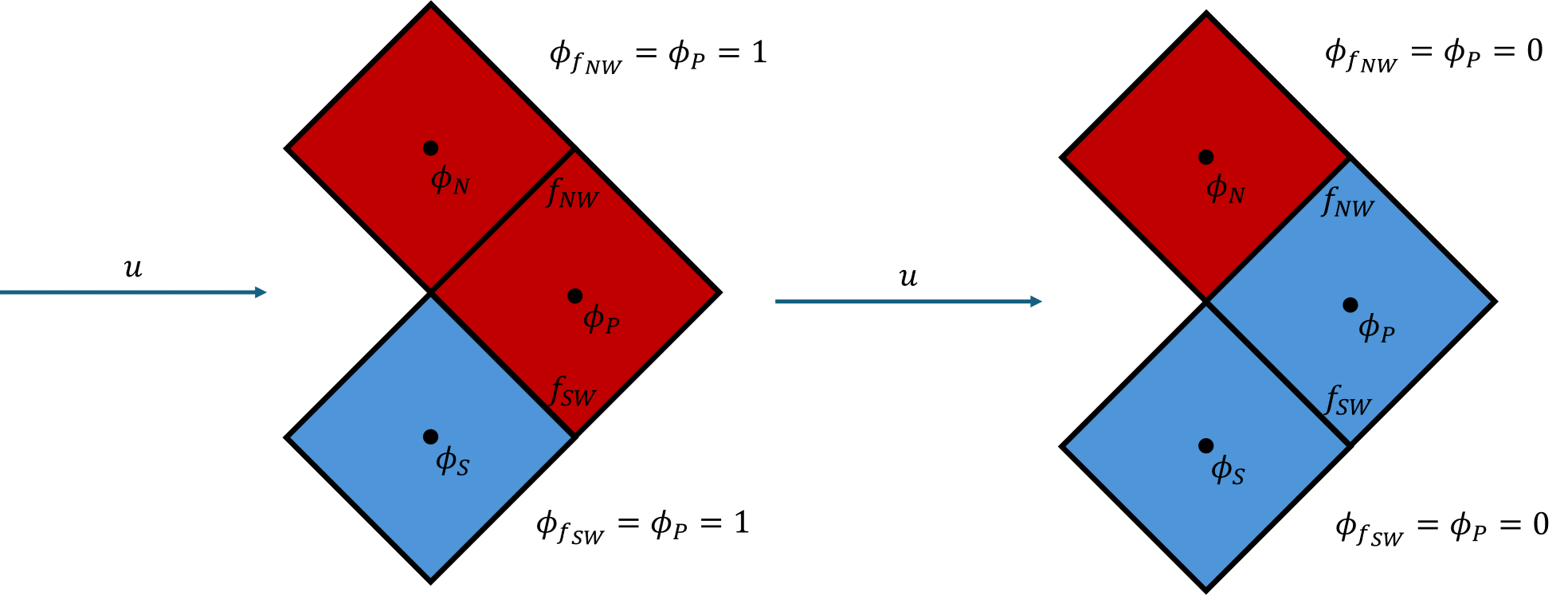
When we initialise the values of [katex]\phi[/katex] at each centroid, we have to make a decision as to which value to take, i.e. either 0 or 1. As the interface goes directly through some of the centroids, the choice here is arbitrary, and the values are set at random.
In the case the values are initialised to 1, then we see on the left-hand side of the figure above that this will result in a value of [katex]\phi_{f_{SW}}=\phi_P=1[/katex].
Thus, when we perform the summation as indicated in Eq.(40), there will be at least one face for which we have [katex]\phi_f=1[/katex]. Even though the cell to the south, as indicated with the centroid value of [katex]\phi_S[/katex], is below the interface, it still feels some influence of the values of [katex]\phi[/katex] from above the interface. This is purely through the influence of the upwind scheme.
We can see the same effect on the right-hand side of the figure, only now some of the values of [katex]\phi[/katex] below the interface are contaminating the solution above the interface. This mixing is, again, numerical diffusion, and the result of using an upwind scheme and having flow misalignment between the bulk flow and the normal vectors of faces.
We can simulate this case as well, which I have done and shown below. On the left-hand side, the bulk flow is aligned with the normal vectors (either parallel or perpendicular), while on the right-hand side, the domain was rotated by 45 degrees. In both cases, the diffusion strength is set to [katex]\Gamma = 0[/katex]. Thus, any diffusion we see is purely numerical.
I have also included a third case, shown in the middle, where I have set [katex]\Gamma > 0[/katex], just to show what physical diffusion would look like in the case of perfect alignment between the bulk flow and the normal vectors.
Below the three cases is a line plot which shows the values of [katex]\phi[/katex], taken on a line going from the bottom to the top of the domain. This line is located in the middle of the domain.
As we can see, the case on the right-hand side, even though there is no diffusion in the equation, it produces the same diffusive behaviour as seen for the case in the middle, where we have physical diffusion. They are indistinguishable. Let's consider why this is important. For this, we'll look at the following figure showing a typical structured and unstructured grid:
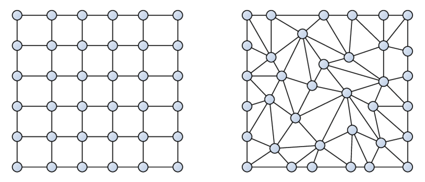
Imagine the flow coming from the left, and then the structured grid would yield no numerical dissipation due to grid misalignment. For the case on the right, however, we would get numerical dissipation in pretty much every cell. Thus, unstructured grids with triangular (2D) or tetra (3D) elements introduce numerical dissipation even if the flow is uniform and only flowing in one direction.
So, what is the influence of the unstructured grid? Well, Grid Pro made a nice comparison in their blog Do mesh still play a critical role in CFD? The following images are taken from their blog post. They considered two separate cases, but I am only going to concentrate on the first one, where they looked at the flow around a NACA 0012 airfoil. They generated several grids, which are shown below (with shockingly low resolution; someone needs to tell them how to unlock full HD resolution ...)
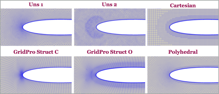
We have different approaches here for the meshing, and these represent common approaches taken these days by commercial and open-source mesh generators. If we look at the results, where the lift coefficient was obtained for different angles of attacks, these turn out as follows:
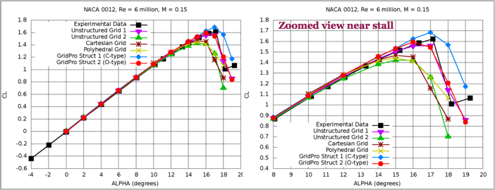
The plot on the right shows a zoomed-in version of the left plot around the angle of attack at which the flow separates and stall appears. Unsurprisingly, the Grid Pro generated grids (the O-grid in particular) perform the best (*cough*), but the point here is that they used structured grids, where the normal vectors were mostly aligned with the flow. Sure, there will be some misalignment, but overall, it will have the least compared to other grids, and the results reflect this.
That is the beauty of structured grids and the reason people still go to great lengths to generate them, even when unstructured grids are far easier to generate!
Strategies to control the numerical dissipation
Now that we have seen how numerical dissipation comes about, it is time to look at some mitigation strategies to see how we can avoid it. Sometimes, we want to have some numerical dissipation, typically to stabilise the flow when our simulations are diverging, but if divergence isn't an issue, we'd like to reduce numerical dissipation to a minimum so as to recover a high accuracy in our simulation. This section will look at steps we can take to achieve just that!
Using higher-order and high-resolution numerical schemes
The simplest strategy to employ is to use a higher-order or a high-resolution numerical scheme. As a rule of thumb, the higher the order of a numerical scheme, the lower the numerical dissipation.
In the grid misalignment case we considered above, I used a first-order upwind scheme as an example. However, second-order, third-order, and even higher-order upwind schemes can be easily constructed. Using one of them will reduce the numerical dissipation, but upwind schemes are prone to adding excessive numerical dissipation compared to other numerical schemes of the same order.
Instead of using a higher-order scheme, you may also want to employ a high-resolution scheme. The definition of a high-resolution scheme is that it is at least second-order accurate (in flow regions without any discontinuities) and that it is free of oscillations around discontinuous signals, though the order may drop to first-order in this region.
Typical examples of high-resolution schemes are MUSCL, TVD, ENO, WENO, and ADER schemes. This list is not exhaustive but these are the ones you likely encounter in the wild (the literature on numerical schemes to capture the non-linear term in the Navier-Stokes equation is vast and many specialised schemes exists).
In contrast, higher-order schemes only have to be at least second-order accurate, but they may oscillate around discontinuities. Typical examples are upwind-based schemes (upwind, Power law, QUICK). These can be combined with flux limiters (such as the minmod, van Albada, van Leer, or superbee limiter) to make them TVD (total variation diminishing), i.e. we can transform a higher-order scheme into a high-resolution scheme, though this does not work with all schemes.
One exception to the norm is central schemes with some numerical dissipation added to them. There are a few proponents, one of the more popular ones being the JST (Jameson-Schmidt-Turkel) scheme. While central schemes are typically unstable, this scheme is stablised by adding numerical dissipation explicitly. Thus, if we have direct control over the numerical dissipation by specifying a numerical value for it in our flow setup, we can arbitrarily reduce or increase it to get stable yet accurate results.
There is a whole class of similar and related numerical schemes, and you can find a good review of them in a report published by NASA.
On the time integration side of things, we have a few options available as well. In particular, multi-step schemes are very commonly used. Multi-step method evaluate the same equation several times, and in the process, subsequently refine the solution. This process is time consuming, but each additional step will enhance the overall accuracy. This is particularly useful for scale-resolved turbulence simulations (DES, LES, and DNS), where accuracy in time is a must.
Of these, the Runge-Kutta family (see this example for a full walkthrough) of time integration schemes is one of the more popular choices. It can be formulated as either an explicit or implicit time integration scheme, and we can add as many steps as we like, increasing the numerical order in the process.
However, each added step significantly increases the computational cost, so a balance between computational efficiency and accuracy is to be found. For explicit time integration, the 4th-order Runge-Kutta version is commonly used, though there is a 3rd-order scheme available that exhibits TVD properties (see Eq.(3.3) in the linked article), which is something we quite like in CFD, especially for compressible flows. An excellent review of implicit Runge-Kutta methods can be found over at NASA again.
For completeness, I shall mention the Adam-Bashforth scheme as well here, which is another multi-step method and sometimes used in CFD. I have only ever seen it implemented in one code, but the name comes up more frequently in literature, so I thought of giving it an honourable mention here as well.
Thus, our choice of numerical schemes will have a direct influence over how much dissipation is added. The better accuracy these higher-order or high-resolution schemes achieve is in part explained by their ability to reduce excessive numerical dissipation.
Using adaptive mesh refinement
We saw above that the grid resolution plays an important role when it comes to numerical dissipation. We looked at a simple example and said that lowering the grid resolution is akin to taking the average of several cells and lumping all of their individual contributions together. We also said that this is exactly the same behaviour any second-order partial differential will do, and thus, we could see the link between numerical dissipation and physical diffusion.
A strategy to circumvent this issue is to locally refine your mesh in areas where the gradients are strong. This is shown in the following figure, where the mesh has been locally adapted to capture the shock waves around the geometry with higher accuracy.

The idea behind adaptive mesh refinement is that if the gradients are strong, the flow must undergo rapid change, and we probably want to refine our flow in this region. This works well if our mesh has a good grid density, to begin with, but if we start with a very coarse mesh, we may not even be resolving any gradients, and thus, adaptive mesh refinement may fail. We saw that in a previous figure, reproduced here for convenience:
We said that the black solid line is the true physical solution, while the dashed lines represented approximation on different grid levels. If the vertical blue dashed lines represent our computational grid, then we obtain a solution as shown by the orange dashed line. This captures the gradient on the right to some extent, so adaptive mesh refinement would pick up this strong gradient and refine the mesh in this region.
If we coarsen the mesh, however, and use only every second grid point, then we obtain the solution shown by the green dashed line. The strong gradient of the physical solution is no longer captured. If we throw adaptive mesh refinement at the green dashed line, the gradients on the left-hand side of the curve are likely stronger, and so we will improve the resolution in an area that doesn't need improvement.
Thus, adaptive mesh refinement can help on grids that have already a good resolution to further tune the accuracy, but they are not a magical solution to throw at every problem. If it was, then it would not be one of the unsolved questions in NASA's 2030 CFD vision.
Using mesh refinement studies
In order to establish a grid on which solution properties of interest do not change anymore, a systematic grid convergence study needs to be done. This provides us with the grid-induced uncertainty, and keeping this low helps us to have more confidence in our solution. If we combine a low uncertainty in the grid with adaptive mesh refinement, we have better chances of succeeding to remove numerical dissipation.
There are challenges around grid convergence studies, especially when it is done incorrectly. In a nutshell, we can manipulate the grid convergence index (the measure of uncertainty) to give us a low reading, even if the real uncertainty is high. It would be too much to get into depth here again. But if you are interested, I have a dedicated article on grid convergence studies and common pitfalls to avoid, which details all of these problems.
Using a structured grid in areas of low numerical dissipation requirements
We saw in the previous section that a structured grid has superior behaviour when it comes to avoiding grid-induced numerical dissipation (which also goes under the name of false diffusion). This means that by using a structured grid, we may be able to avoid adding some diffusion in areas where it would have unfavourable consequences.
Take the flow around a wing. Without any treatment at the wingtip, and assuming that we have a lower pressure on the top than on the bottom of the wing (i.e. we are generating lift), then we will get a vortex forming around the wing tips, as demonstrated in this streamline visualisation of a CFD simulation:
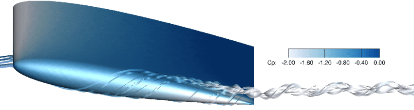
If you are tasked with capturing this vortex downstream, you'd be surprised how quickly this vortex dissipates if you don't have a really good grid resolution here. I had a student who had the (dis)pleasure of investigating exactly this phenomenon, and even after a few months of work, we weren't able to get results with an unstructured meshing approach (this included a proper grid convergence study and adaptive and local mesh refinement). It came down to creating a structured mesh, which finally solved the issue.
You don't have to create a completely structured mesh; you can also insert only locally structured meshing regions if your mesh generator allows it. Mesh the regions with a structured mesh where you absolutely require a nicely flow-aligned structured grid and reap the benefits of low numerical dissipation.
Depending on your mesh generator, you will pay the price (mainly in the form of insanity) to generate a mesh (depending on geometric complexity). Happy meshing!
Using numerical dissipation to our advantage
Up to this point, it may seem that numerical dissipation is a pest, and we need to eliminate it as best we can. But this would be beside the point. Numerical dissipation is extremely important in stabilising our numerical simulations and, in some cases, can be used to match physical dissipation, which may have been lost through modelling assumptions. Thus, in this section, it's time to show some love and appreciation for a quantity that is often misunderstood.
Turbulence modelling
Turbulence modelling is one of the greatest challenges in CFD! If all you did was to perform some RANS simulations in a commercial CFD solver, then you would likely think that turbulence modelling is a solved issue. Just use the [katex]k-\omega[/katex] SST RANS model, and you are good to go, right?
When I interviewed for my PhD position, I remember getting into an argument with one of the post-docs who was working in the wind tunnel. He tried to convince me that turbulence modelling was hard, that boundary conditions are a tricky business, especially for direct numerical simulations, but I just kept insisting that turbulence modelling was rather straightforward. There was a time I believed that, but then I started running DNS and large-eddy simulations (LES), and I realised that he was right!
Boundary conditions are just one of many issues that arise in turbulence modelling, but let's conceptually review the differences in the main modelling strategies. We have Reynolds-averaged Navier-Stokes (RANS), as well as the aforementioned LES and DNS. If we were to simulate the flow of a jet, using either of these approaches may result in the following contours for the velocity magnitude:
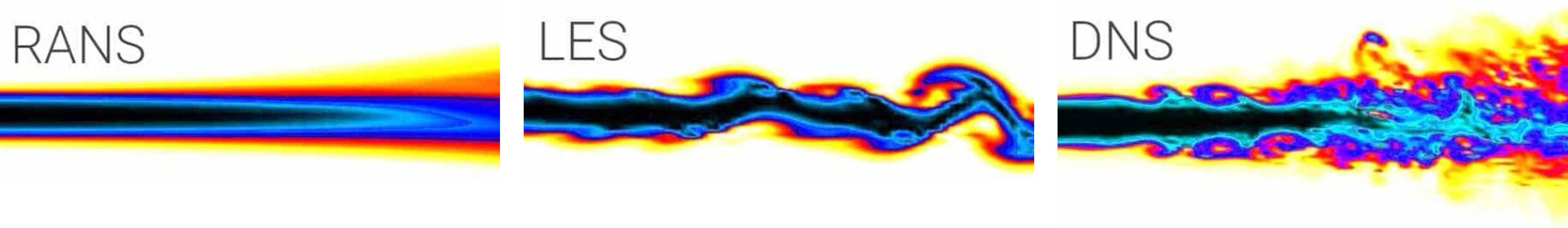
RANS provides us with a time-averaged result; thus, we get a smooth contour profile. Both LES and DNS provide us with time-resolved results, and thus we start to see some of the fluctuations that appear over time. More so in DNS than LES, which is also shown in the following figure:
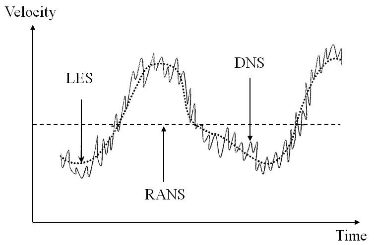
We see that taking the velocity signal over time at some point in the flow will give us an average for RANS (flat line), while LES captures the bulk movement. LES can't, however, resolve all of the small-scale fluctuations which appear in DNS simulations. Going from RANS to LES and from LES to DNS increases the computational cost significantly. In particular, we say that the computational cost scales as follows:
- RANS: [katex]~Re[/katex]
- LES: [katex]Re^2--Re^2.5[/katex]
- DNS: [katex]~Re^3[/katex]
Let's take an example. If we assume that we can perform a simple airfoil simulation at a Reynolds number of 1 million with RANS that takes about 5 minutes to compute, we can calculate how much longer that would take for LES and DNS. In this example, an LES simulation would take around:
\frac{LES_{cost}}{RANS_{cost}}RANS_{time}=\frac{Re^2}{Re}5 \,\mathrm{min}=10^6 \cdot 5\,\mathrm{min}\approx3472 \,\mathrm{days}\tag{43}If we now use high-performance computing (HPC) and a total of 1024 cores, we can get results with LES in about 3.4 days. For DNS, it is looking even worse:
\frac{DNS_{cost}}{RANS_{cost}}RANS_{time}=\frac{Re^3}{Re}5 \,\mathrm{min}=Re^2\cdot 5 \,\mathrm{min}=10^{12} \cdot 5\,\mathrm{min}\approx 10^7 \,\mathrm{years}\tag{44}Even if we were to use [katex]10^7[/katex] processors (assuming we have access to an HPC cluster that has a sufficient number of cores available and we are able to use all of them), we would still have to wait for a year to get our results. If we compare the steep increase from 5 minutes for a RANS simulation to one year using 10 million processors to get DNS resolution (resolving all turbulence scales, not making any modelling assumptions), we can quickly see the need to model at least some of the turbulence.
Let's view turbulence in terms of length scales. We saw above that by going towards DNS, we start to resolve smaller and smaller scales. The following figure shows how the turbulent kinetic energy changes over smaller and smaller length scales.
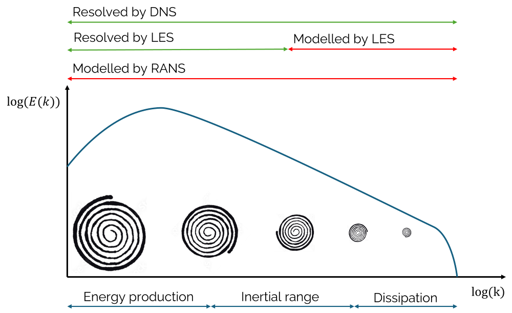
Here, the x-axis is in terms of the wave number [katex]k[/katex], which is the inverse of the length scale. Thus, as we move on the x-axis towards the right (higher wave numbers), the length scales decreases. I have shown this here by indicating that the turbulent eddies we would see in the flow are decreasing in size as we go to the right.
We can now categorise the flow into 3 separate regions. On the left, that is, for the smallest wave numbers and thus largest length scales, we have the energy production range. The turbulent eddies are produced here by the non-linear term in the Navier-Stokes equations, and they have the largest length scales. We can see schematically shown above the figure that both LES and DNS are resolving these scales, and this is what we were able to see in the figures above as well.
On the right, we have the dissipation range. This happens at the smallest length scales (highest wave numbers). Only DNS resolves these, while LES attempts to model them. In between the energy production and dissipation range, we have the inertial range, which follows a linear decay. Well, this is a log-log plot, so what we see as a linear decay here is, in reality, an exponential decay. This decay can be shown to follow an exponential function with the exponent of -5/3, a highly celebrated universal law in turbulence research due to Kolmogorov.
We see that only DNS is resolving this entire spectrum. Thus, in order to capture the smallest scales (high wave numbers towards the right of the plot), we need to have a sufficiently fine grid to capture the smaller and smaller length scales. This is where the cost of DNS is coming in. The grid requirements in terms of grid points required are astronomically high.
At the same time, we see that both LES and RANS model the turbulent structures at the dissipation range. In other words, we can make our grid much coarser compared to DNS, but doing so removes the smallest scale that dissipates turbulence into heat.
The scale that we do resolve, though, is the largest energy-containing one with LES, while RANS attempts to model these. Well, RANS captures some of that large energy, just not in a temporal sense (due to its time-averaging nature). Where does this energy come from? Simply put, we have some kinetic energy in our flow that is transformed from (laminar) kinetic energy into turbulent kinetic energy.
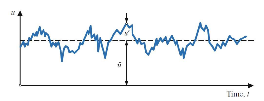
To see where it comes from, let's consider Reynolds' original velocity decomposition. Reynolds postulated that every instantaneous velocity signal can be decomposed into two parts: its time average and a fluctuating velocity component:
\underbrace{u}_{\mathrm{instantaneous}}=\underbrace{\overline{u}}_{\mathrm{average}} + \underbrace{u'}_{\mathrm{fluctuations}}\tag{45}This is also schematically shown in the following figure:
Let's consider the non-linear term in the Navier-Stokes equation, i.e. [katex](u\cdot\nabla)u[/katex]. We can expand it for the [katex]x[/katex], [katex]y[/katex], and [katex]z[/katex] direction as follows:
- [katex]x[/katex] momentum equation:
\frac{\partial uu}{\partial x}+\frac{\partial uv}{\partial y}+\frac{\partial uw}{\partial z}\tag{46}- [katex]y[/katex] momentum equation:
\frac{\partial uv}{\partial x}+\frac{\partial vv}{\partial y}+\frac{\partial vw}{\partial z}\tag{47}- [katex]z[/katex] momentum equation
\frac{\partial uw}{\partial x}+\frac{\partial vw}{\partial y}+\frac{\partial ww}{\partial z}\tag{48}In order to see where the turbulence is generated, we need to introduce Reynolds' decomposition. For two quantities [katex]a[/katex] and [katex]b[/katex], this can be written as:
\frac{\partial ab}{\partial x}=\frac{(\overline{a}+a')(\overline{b}+b')}{\partial x}=\frac{\overline{a}\overline{b}}{\partial x} + \frac{\overline{a}b'}{\partial x} + \frac{a'\overline{b}}{\partial x} + \frac{a'b'}{\partial x}\tag{49}Let's consider the time-averaged form of this Reynolds decomposition.
\frac{\partial \overline{ab}}{\partial x}=\frac{\overline{(\overline{a}+a')(\overline{b}+b')}}{\partial x}=\frac{\overline{\overline{a}\overline{b}}}{\partial x} + \frac{\overline{\overline{a}b'}}{\partial x} + \frac{\overline{a'\overline{b}}}{\partial x} + \frac{\overline{a'b'}}{\partial x}\tag{50}The average of an average is just the average itself, so the first term remains as it is. The second and third terms go to zero, as the average of the fluctuating velocity component is, by definition, zero ([katex]a[/katex] and [katex]b[/katex] are just placeholders for velocity components).
Look at the figure above; if we remove the average velocity field from the fluctuating velocity component, then we would get velocity fluctuations centred around a zero velocity. Integrating over time (taking a time average) would result in a velocity value of zero. Thus, the second and third velocity components are zero.
The fourth velocity component, on the other hand, is not zero. Therefore, we can write the non-linear term in the Navier Stokes equations as follows:
- [katex]x[/katex] momentum equation:
\frac{\partial uu}{\partial x}+\frac{\partial uv}{\partial y}+\frac{\partial uw}{\partial z}+\frac{\partial\overline{u'u'}}{\partial x} + \frac{\partial \overline{u'v'}}{\partial y}+\frac{\partial\overline{u'w'}}{\partial z}\tag{51}- [katex]y[/katex] momentum equation:
\frac{\partial uv}{\partial x}+\frac{\partial vv}{\partial y}+\frac{\partial vw}{\partial z} +\frac{\partial\overline{u'v'}}{\partial x} + \frac{\partial \overline{v'v'}}{\partial y}+\frac{\partial\overline{v'w'}}{\partial z}\tag{52}- [katex]z[/katex] momentum equation
\frac{\partial uw}{\partial x}+\frac{\partial vw}{\partial y}+\frac{\partial ww}{\partial z} +\frac{\partial\overline{u'w'}}{\partial x} + \frac{\partial \overline{v'w'}}{\partial y}+\frac{\partial\overline{w'w'}}{\partial z}\tag{53}To see that these additional quantities, the so-called Reynolds stresses, are not equal to zero, and this is best seen by measuring them in a flow. For example, the following plot shows measurements of [katex]u'u'[/katex], [katex]u'v'[/katex], [katex]v'v'[/katex], and [katex]w'w'[/katex] (which are written as [katex]<uu>[/katex], [katex]<uv>[/katex], [katex]<vv>[/katex], and [katex]<ww>[/katex]). They were measured near a wall, which created a boundary layer profile.
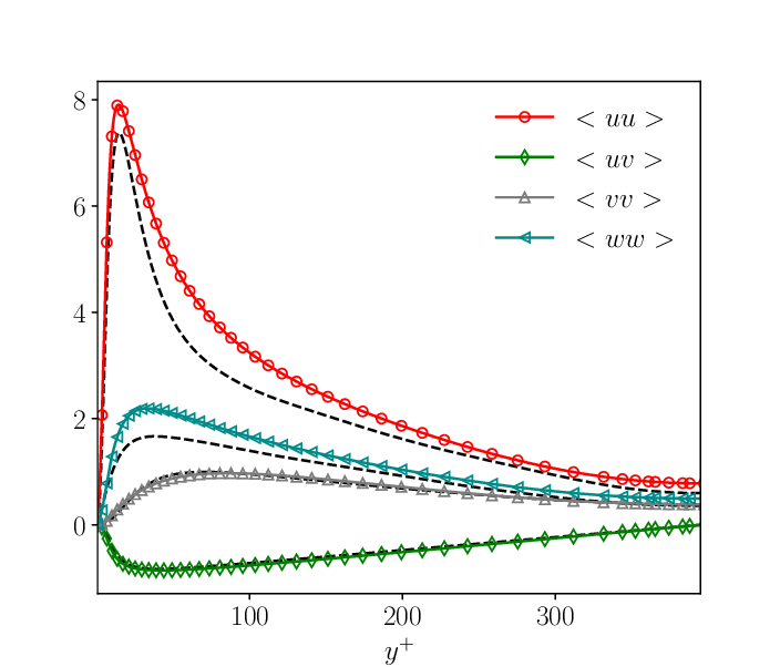
We can see that the Reynolds stresses are not equal to zero even far away from the wall (large [katex]y^+[/katex] values). It is precisely these additional terms in the Navier-Stokes equations which generate turbulence by converting (laminar) kinetic energy into turbulence kinetic energy.
The stronger the gradients, the stronger the Reynolds stresses, and thus, we see turbulence being generated in regions of high gradients. These typically appear in boundary layers, where the velocity has to be zero at the wall due to the no-slip condition but equal to the freestream velocity close to the wall. This creates large velocity gradients that drive the generation of turbulence, and the reason our boundary layer goes through a laminar, transitional, and then fully turbulent phase.
Thus, we can see that turbulence is generated by the non-linear term, and the role of turbulence modelling (e.g. RANS) is to find suitable values for these Reynolds stresses. The source of turbulence generation is, therefore, explicitly included in the equation.
Even if we consider a DNS, where the equations are not changed (no Reynolds stress terms are included), since we are resolving all fluctuations, we could manually decompose the velocity field into a mean and a fluctuating velocity component in each cell and recover the Reynolds stresses. In fact, when dealing with DNSs, this is commonly done to compute other quantities of interest, such as the dissipation rate.
OK, we know from high-school physics that whenever we are generating something out of "thin air" (here, turbulence), we have to balance it by destroying it (well, in high-school physics we learned that energy can't be created nor destroyed, it can only change its type. Here, we have conversion of laminar into turbulence kinetic energy).
So how does turbulence get destroyed? (how does it change its energy type and into what quantity?) Surely, we can all agree that all generated turbulence eventually has to go away if not sustained by an external energy source. If you stir your tea or coffee and then stop, eventually, the fluid will come to rest, and all turbulence you generated in your cup will go away. But how?
Well, this is where our energy cascade comes back from what we saw above. Let's look at that again:
At the smallest length scales (high wave numbers [katex]k[/katex]), all turbulence kinetic energy [katex]E(k)[/katex] is dissipated into heat. The term dissipated provides the clue. It is the diffusion term in the Navier-Stokes equations, i.e. [katex]\nu\nabla^2 \mathbf{u}[/katex], which is responsible for removing any small-scale turbulence and dissipates that into, well, heat. So energy is conserved, and our high-school physics teachers can sleep again at night (we learned that law of energy conservation correctly), but where does that leave us in our current discussion?
Well, looking at the figure, we see that only DNS resolves all scales. DNS can resolve the generation of turbulence at the largest length scales (low wave numbers), which we discussed are generated through the Reynolds stresses. Then, the flow goes through the energy cascade, where the energy contained in the turbulent flow is steadily decreased until we reach the smallest scales, where DNS dissipates that into heat.
LES can't resolve the smallest scales and, by definition, is designed in such a way that it captures all of the energy production range and most of the inertial range. So how does LES dissipate heat at the smallest scales? Well, this is where the sub-grid scales (SGS) model comes in. The SGS model provides the lost dissipation and thus balances the energy cascade again.
And for RANS? Well, everything is essentially modelled, and we can see that RANS turbulence modelling is nothing else than adjusting the amount of diffusion in our system. Boussinesq's eddy viscosity hypothesis states that the Reynolds stresses can be equated to mean flow gradients (strain rate tensor). Boussinesq's hypothesis reads:
\tau_{ij}=2\mu_t S_{ij}-\frac{2}{3}\rho k \delta_{ij}\tag{54}Here, the indices for [katex]i[/katex] and [katex]j[/katex] are 0, 1, and 2, representing the [katex]x[/katex], [katex]y[/katex], and [katex]z[/katex] direction. The Reynolds stresses are given by [katex]\tau_{ij}[/katex] and inserting, for example, [katex]i=1[/katex] and [katex]j=2[/katex] would result in [katex]\tau_{ij}=\tau_{12}=v'w'[/katex]. [katex]S_{ij}[/katex] is the strain rate tensor, [katex]\rho[/katex] is the density, [katex]i[/katex], [katex]k[/katex] is the turbulent kinetic energy, and [katex]\delta_{ij}[/katex] is the Kronecker delta.
If you see this for the first time, don't worry; you don't need to understand how this term comes about. The only thing that is important here is that the strain rate tensor is scaled by the turbulent eddy viscosity [katex]\mu_t[/katex]. It is the role of any RANS model to obtain this value. Then, you may find that your diffusive term in the Navier-Stokes equation is then written as
(\mu+\mu_t)\nabla^2 \mathbf{u} = \mu_{eff}\nabla^2\mathbf{u}\tag{55}Thus, a RANS model adds more diffusion to our system to balance the energy cascade and the dissipation effect that we lost at the smallest scales. We need to do this, as the grid for a RANS turbulence model is too coarse to resolve any of these effects. Thus, by simply tuning the diffusion with some additional turbulent viscosity, we can locally scale our diffusion to match the dissipation lost at the smallest scales.
You are probably already getting ahead and seeing how all of this comes back to numerical dissipation. I stated in the beginning that we need numerical dissipation in order to stabilise our flow, and this is exactly the reason why we need to do that. If we do not add numerical dissipation, using either a numerical scheme or modelled dissipation coming from a RANS or SGS model, then we bring our system into imbalance.
When you have more turbulence being generated at the largest scales, but then you don't have enough dissipation being added back to the system, your simulations will start to diverge (there are many different reasons for divergence; this is just one of them, i.e. if you encounter divergence next time, it may not necessarily be due to missing dissipation, but typically we add more dissipation to see if that stabilises the flow again).
Having said all that, we saw that there are rather striking similarities between numerical dissipation being added by a numerical scheme and modelled dissipation (diffusion) being added by a RANS or SGS model. What is stopping us from using numerical dissipation to replace either a RANS or SGS model?
The answer is nothing, and this is what people are doing. We can create a so-called Implicit Large-eddy Simulation, or ILES, where the SGS model is removed and we hope that the numerical dissipation alone is sufficient to capture the dissipation from the smallest of scales in the turbulent flow. Sometimes, ILES is also called a coarse or under-resolved DNS, and the name makes sense. The equations are the same as for DNS, we just use a coarser grid which doesn't resolve all scales.
I've always stated that the simplest turbulence model is the first-order upwind scheme. Upwind schemes add excessive dissipation, as we saw above when we looked at grid misalignment and how upwind schemes start to add diffusion. The only problem with this idea is that upwind schemes do not provide us with a mechanism to scale the dissipation. So, while they add dissipation, similar to a RANS model, it isn't a very accurate approach as we have no control over the amount of numerical dissipation.
And there you have it: numerical dissipation is crucial for balancing the production and destruction of turbulence if we want to avoid divergence. But there is more. Numerical dissipation helps not only with turbulence but also with compressible flows. Let's look at that next.
Shock-capturing methods
It is fair to say that the early days of CFD were concerned with finding ways to capture the strong gradients that arise in the Navier-Stokes equations through sophisticated numerical schemes (sophisticated for the 1950s, by today's standard they are rather straight forward, at least compared to some of the more advanced schemes we have nowadays).
First, we used the simple advection equation we saw above in the modified equation analysis, and then later, the non-linear version (Burgers equation). Eventually, we ventured into solving the (inviscid) Navier-Stokes equations, also known as the Euler equation. Regardless of the equation being solved, numerical scheme development was the name of the game. More sophisticated schemes were introduced, and the fact that CFD can seem so easy (if you are using a commercial solver) is thanks to the research efforts that have been carried out at this time.
When we talk about the Euler equation, we do not consider any physical dissipation. The equations can be written in conservative form as:
\frac{\partial \mathbf{u}}{\partial t}+\nabla(\mathbf{u}\otimes \mathbf{u})=-\frac{1}{\rho}\nabla p\tag{56}This equation is inviscid, meaning that there are no boundary layers that we need to resolve (turbulence is not considered here). However, while we saw in our discussion above that Reynolds stresses appear in region of strong gradients (boundary layers) which then need to be modelled, resulting in additional dissipation through either a RANS or SGS model, we still have strong gradients in the Euler equations, even without considering turbulence. And these are generated in regions where we have shocks.
A shock wave is, mathematically speaking, a discontinuity. Since the Navier-Stokes equations are typically given in differential form, we can see how discontinuities can pose problems. The derivative of a discontinuous function is infinity. This is rather challenging to deal with, and so typically, we transform the Navier-Stokes equation into an integral form, where we replace derivatives with integrals where we can.
Let's consider the Euler equation again, but now say that the pressure is constant in our flow, i.e. its gradient is zero everywhere. We obtain the following equation:
\frac{\partial \mathbf{u}}{\partial t}+\nabla(\mathbf{u}\otimes \mathbf{u})=0\tag{57}This is known as the Burgers equation. Yes, back in the day, you could take the Navier-Stokes equation, chop off bits and pieces, and then have whatever is left of an equation named after you. In 1D, we can write this equation in scalar form as:
\frac{\partial u}{\partial t}+\frac{\partial uu}{\partial x}=0\tag{58}If we now assume that we have an initial condition of [katex]u(x,t=0)=sin(x)[/katex] and we use Eq.(58) to solve it, then, after some time, we get the following results for the profile:
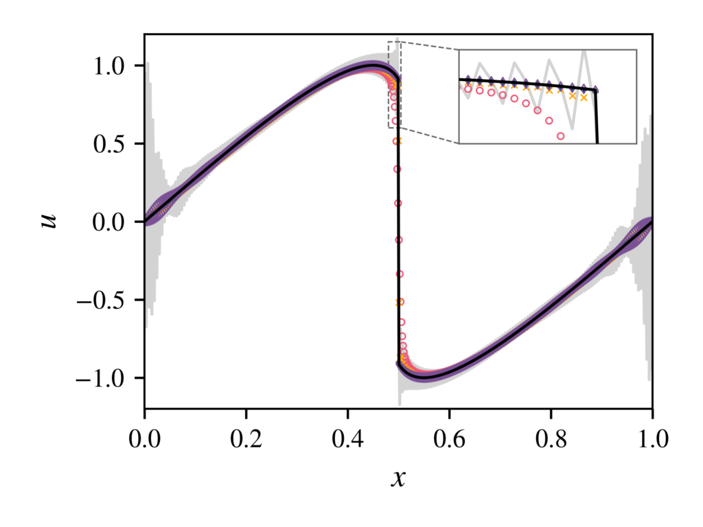
If we concentrate on the profile at [katex]x=0.5[/katex], we can see at the top right that the exact solution (solid black line) is approximated well by the solution provided by the red circles (some unspecified numerical scheme for now). Looking at the solid black line again, we can clearly see where a discontinuity is present. The solution using the numerical scheme indicated by the red circles has to provide some smoothing around the discontinuity to be able to resolve it.
This smoothing is, again, due to numerical dissipation. Thus, the solution of the red circles may be obtained using an upwind scheme, for example. The smoothed solution will have finite gradients again, which makes the problem easier to solve from a mathematical point of view (gradients are no longer going to infinity).
If we keep the numerical dissipation low, or, try to remove it altogether, then we get a behaviour that is similar to that shown by the grey solid line. We generate lots of over- and under-shoots. If they are strong enough, they can induce divergence.
This behaviour is problematic for another reason. Consider the case of the density. Let's say we try to approximate a discontinuity where the density is small on one side of the shock. If the over- and under-shoots are larger in magnitude than the density itself, we will obtain negative values for it locally. The density can't be negative, though, and this non-physical behaviour is a pure side-effect of the numerical scheme. Again, we'd rather deal with numerical dissipation than with numerical schemes that violate physical conservation laws!
A negative density may be the cause for locally induced divergence as well, so this is another reason we would like to avoid it. Furthermore, while we think of shock waves as discontinuities, they are only discontinuous to us humans. In reality, shock waves have the following structure:
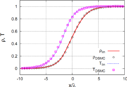
Here, we see values for the non-dimensional temperature and density across a shock wave. it looks rather smooth, doesn't it? Well, that is because the x-axis is now normalised by the mean-free path [katex]\lambda[/katex], i.e. the distance a molecule travels (on average) before hitting another molecule. For air at room temperature, this value is [katex]\lambda\approx 6.5\cdot 10^{-8}[/katex] meters. Thus, we can see that the shock thickness is ranging between [katex]-5\le x/\lambda \le 5[/katex], or about [katex]6.5 \cdot 10^{-7}[/katex] meters.
So, if we were to refine our mesh to have a mesh resolution of the order of [katex]\lambda[/katex], does it mean that we get the same smooth shock wave structure? Not quite. The Navier-Stokes equation is based on the continuum assumption; that is, we assume that we can describe the flow as a collective behaviour of the underlying particles. The figure above used the Direct Simulation Monte Carlo method (DSMC), which is based on a particle description. Therefore, it is able to resolve the shock wave smoothly.
Thus, numerical dissipation, again, mimics reality, just as we saw in the case of turbulence. In this case, though, shock waves (discontinuities) are smoothed excessively compared to the real thickness of shock waves.
Case study - Using low-dissipative numerical schemes to break the Navier-Stokes equations
We have looked now at how numerical dissipation comes about and why it is such a useful member of society! In this section, I want to put all of our discussion to the test and show you how all of this plays out in the real world. For this, we are going to consider the world's simplest geometry, a square domain on a Cartesian grid. All sides will have wall boundary conditions, and the only tweak we are doing is to set the top wall in motion by making it slide over the top layer of fluid. This is schematically shown in the following figure:
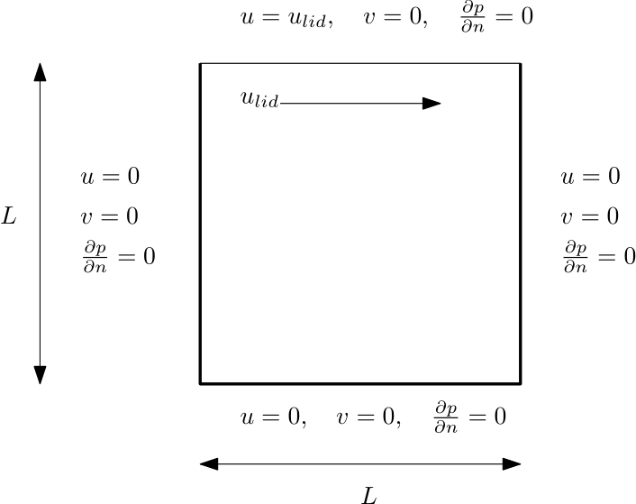
The experts among you will have recognised that I am indeed talking about the lid-driven cavity. This is a classical test case for incompressible flows and one of the first geometries you want to test your own solver on if you are writing one from scratch. The nice thing about this geometry is that the mesh is so simple to generate. You can do that within your solver. Yet, the flow structures that appear can be rather complex, based on the Reynolds number (where the characteristic length here is taken to be the length of the box).
As we set the top wall in motion, a main vortex will form in the middle, as is nicely demonstrated in this animation:
As the Reynolds number increases, smaller secondary, and even tertiary vortices will form in the corners of the domain. Turbulence starts to kick in and all of a sudden we have a complex flow to handle, even with this relatively simple set up.
What I have done is to write a solver that implements the Artificial Compressibility method for incompressible flows. The method is not the best, but it is usually a good method to get started as it is rather straightforward to implement. I have used two numerical schemes to approximate the values on the faces. One scheme is, on purpose, a rather low-dissipative numerical scheme, and given as:
\phi_f=\frac{5}{6}\phi_i - \frac{1}{6}\phi_{i-1}+\frac{1}{3}\phi_{i+1}\tag{59}The low-dissipative nature is obtained by choosing not to use any upwinding at all. As we saw above, upwinding is a typical cause of numerical dissipation. Now, this is a fairly risky strategy, as this will eventually introduce divergence. However, for our current discussion, it means that we are able to see what a low-dissipative scheme will do to our simulation!
The second scheme that I used is the Jameson-Schmidt-Turkel (JST) scheme, i.e. the central differencing approximation with user-defined dissipation. This can be written as
\phi_f=\frac{\phi_i+\phi_{i+1}}{2}+D_i\tag{60}Here, the term [katex]D_i[/katex] adds numerical dissipation explicitly through a second-order and a fourth-order term. It isn't important to understand for our discussion what this term looks like (there are a few steps involved), but if you want to know, look at Swanson et al.'s work (Section 2.1). Suffice it to say that [katex]D_i[/katex] has user-defined parameters that allow us to either increase or decrease the amount of dissipation.
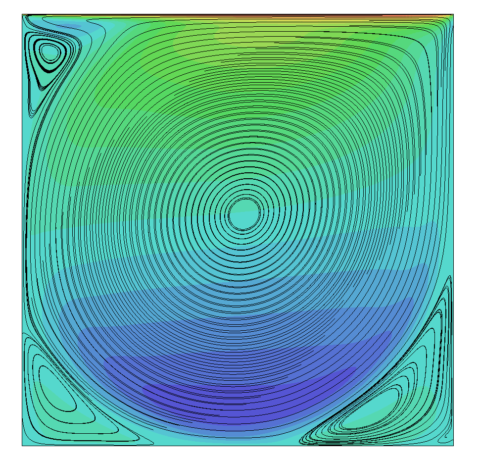
So let's look at some results, comparing the low-dissipation scheme (Eq.(59)) with the JST scheme that is adding numerical dissipation explicitly (Eq.(60)). The following figure shows results obtained for the lid driven cavity at a Reynolds number of [katex]Re=1000[/katex].
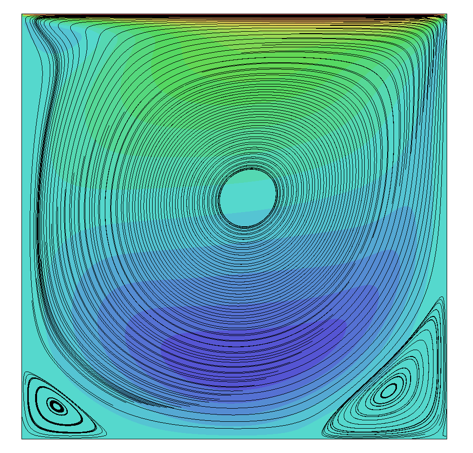
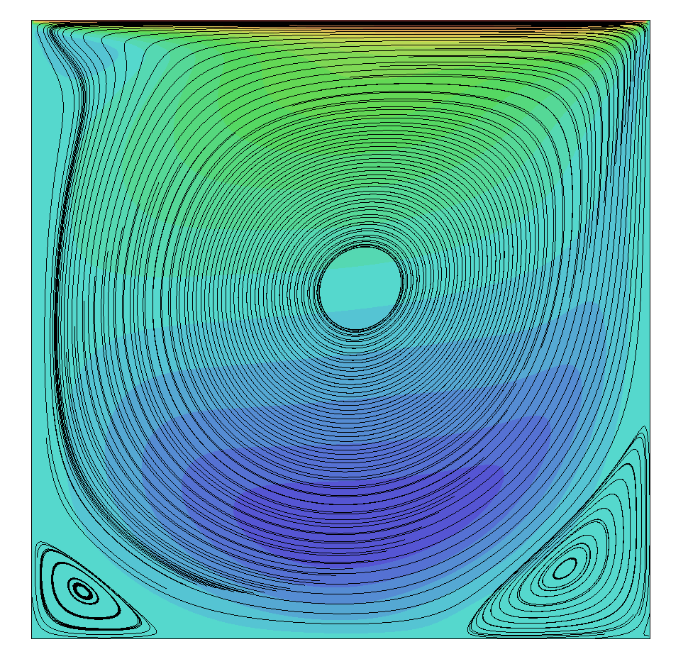
On the left, we see the results for the low-dissipative scheme and and on the right for the JST scheme, i.e. the one with explicit numerical dissipation. Both provide fairly similar results, and both resolve the primary vortex, as well as the secondary corner vortices rather well. So far so good.
But now, let's increase the Reynolds number and see what happens. The results for a Reynolds number of 5000 are shown below:
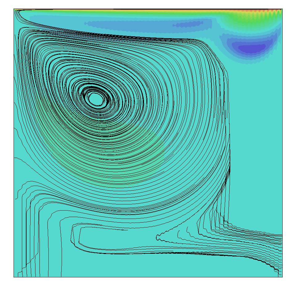
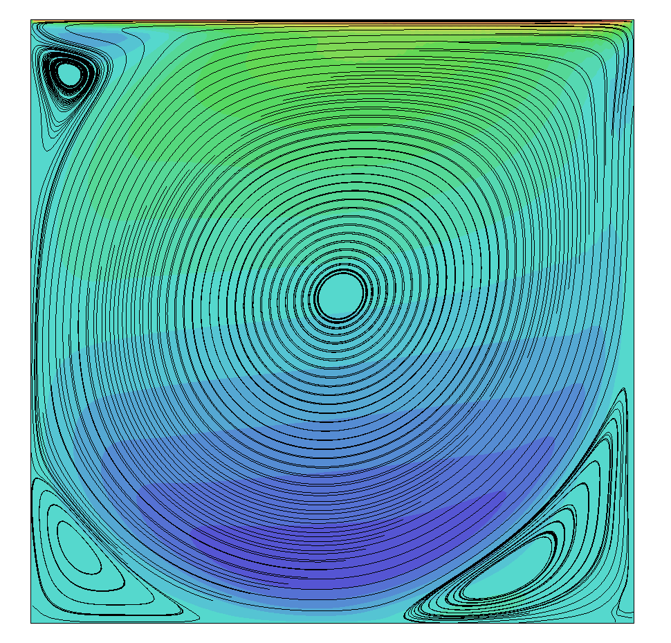
On the left, we see the results obtained with the low-dissipative numerical scheme (Eq.(59)). Compare that with results obtained with the JST scheme and numerical dissipation added (Eq.(60)) shown in the middle. The addition of numerical dissipation has stabilised the flow, while a low-dissipative scheme is unable to obtain physical results.
However, all is not lost. We can reduce the mesh spacing by a factor of two in both the x and y direction, and thus increase the mesh size. The results then obtained with the low dissipative scheme (Eq.(59)) are then obtained as shown in the figure above on the right. All of a sudden, we do get correct results again, can you guess why?
Well, it all comes down to what we discussed in the turbulence section before. Let's review the energy cascade again:
We said that the eddies at the dissipation range dissipate into heat. But what is their size? Well, there is a simple scaling relationship in turbulence modelling that states:
\frac{\eta}{l_o} \sim Re^{-3/4}Here, [katex]\eta[/katex] is the so-called Kolmogorov turbulence length scale, which is the smallest length scale in our flow (i.e. the smallest eddies having the smallest diameter). These are located on the far right in the figure above (not on the political spectrum). [katex]l_o[/katex] is a length scale associated with the largest length scales in the flow, and these are located on the far left in the figure above. These are typically your boundary layer height or similar macroscopic length scales we can easily observe.
In our case, [katex]l_0[/katex] is proportional to the size of the domain, which doesn't change, and thus an increase in Reynolds number produces smaller Kolmogorov turbulence length scales [katex]\eta[/katex]. A smaller length scale means higher wave numbers.
For our discussion, this means that if we use the same mesh size but we increase the Reynolds number, we resolve less of the above-shown energy cascade. Since we resolve less of the energy cascade, we introduce a larger imbalance between energy production and destruction, which at some point leads to divergence (the results we saw above on the left-hand side of the three contour plots).
So, we have now two options. Either, we increase the amount of dissipation through numerical dissipation (e.g. Eq.(60) or a turbulence model), or, we simple resolve more of the energy cascade. To do that, we have to decrease the mesh spacing, so that we can capture smaller scales of our flow. This is what I have done by increasing the mesh size and from the streamlines we saw above, it was evident that this also stabilised the flow.
This is the same reason why you see people doing LES using low-dissipative schemes such as the central difference scheme (perhaps with some limiting), which you would never dream of in RANS simulations. As we decrease our mesh spacing, we resolve more and more of the energy cascade and thus physical dissipation, alleviating the need for highly dissipative (but stable!) numerical schemes such as the upwind method.
Summary and outlook
And so, there you have it. Numerical dissipation is a concept we can't avoid and, as it turns out, don't want to either. Unless you read this post in a few years (decades?!), where we have adopted quantum computing and do direct numerical simulations (DNS) on a daily basis, then numerical dissipation is a concept you need to understand.
Numerical dissipation is a property that is mainly driven by the numerical schemes and computational grid arrangements we use. We saw that upwinding introduces excessive numerical dissipation, but it also stabilises the flow, so we may get away with using an under-resolved grid for fast calculation times. Grid alignment plays another crucial role, and we saw that unstructured grids using triangles (2D) and tetrahedra (3D) are particularly prone to introduce numerical dissipation compared to quad (2D) or hexa (3D) cells (i.e. structured grids).
If we want to reduce numerical dissipation to improve accuracy, we need to either use higher-order or high-resolution numerical schemes or adjust the mesh spacing. Adaptive mesh refinement may be one of the best tools we have to balance the amount of numerical dissipation locally.
However, we also saw that numerical dissipation is vital in helping us to get physical results for flows where we have large Reynolds numbers (turbulence) or high Mach numbers (shock waves). In the case of turbulence, numerical dissipation takes on the role of dissipating turbulent structures that would normally be dissipated at the smallest length scales. If the numerical scheme is doing so now, we no longer need the smallest scales and can simply remove them (i.e. make our grid coarser).
In the case of shock wave capturing, we saw that numerical dissipation smooths out gradients and, in a sense, recovers the true nature of shock waves, which are anything but discontinuous. Shock waves have a smooth transition from one state to another, it just happens to be on a length scale that is too small for our simulation (and, indeed governing equations) to resolve it. So numerical dissipation does, again, recover a correct physical solution, albeit with excessive dissipation in this case. Regardless, the simulation is stabilised as a result.
From now on, I hope you'll appreciate the role of numerical dissipation and the fact that it is always there, somewhere in your simulations, even if you can't see or quantify it (easily).
Think of it as chocolate; a bit of chocolate here and there is fine. But, if you consume too much of it, you'll be on a sugar rush and probably it isn't great for your health either. Our role is to ensure that our simulations undergo a healthy diet. Cut down on chocolate where you can, but don't remove it altogether, or you have a screaming toddler running around the house and throwing toys everywhere (the experts say that the simulation is diverging).
Acknowledgements
Special thanks to Ali Eken for helping me to improve this article! Check out how you can contribute, too.
Tom-Robin Teschner is a senior lecturer in computational fluid dynamics and course director for the MSc in computational fluid dynamics and the MSc in aerospace computational engineering at Cranfield University.