Space and time integration schemes for CFD applications

There are probably as many numerical schemes to solve the discretised Navier-Stokes equations as there are stars in the Milky Way. Well, perhaps a few less. Just have a look at OpenFOAM, and you’ll find over 60 discretisation schemes for the non-linear term in the Navier-Stokes equations. And, while that number seems impressive, I am still missing quite a few schemes in OpenFOAM that have established themselves in the CFD literature.

We can probably reason that we want to use different numerical schemes for various situations. So the goal of this article is to give you a well-rounded overview of which schemes exist in the finite difference method to approximate gradients, in the finite volume method to interpolate variables onto cell faces, as well as for integrating the equations in time.

By the end of this article, you will understand the different requirements we have towards a numerical scheme, as well as which schemes are commonly used in CFD to solve the discretised equations. Put on the kettle, have yourself a nice cup of tea, we are in for a ride, let’s go!

In this series

• Part 1: How to Derive the Navier-Stokes Equations: From start to end
• Part 2: What are Hyperbolic, parabolic, and elliptic equations in CFD?
• Part 3: How to discretise the Navier-Stokes equations
• Part 4: Explicit vs. Implicit time integration and the CFL condition
• Part 5: Space and time integration schemes for CFD applications

In this article

Introduction

Let’s quickly recap where we are in our series. In our first article, we derived the Navier-Stokes equation from start to end, with all the intermediate steps. I know, it was a lengthy article, but a necessary one; usually, the derivation of our governing equation for CFD applications does not get the depth they need and deserve!

Next, we classified the governing equations into hyperbolic, parabolic, and elliptic equations. We saw that the different characters brought about different mathematical behaviours that we can see in the flow field if we know what to look for.

After we derived and classified the governing equations, we looked at how we can discretise the equations using either the finite difference method (FDM) or the finite volume method (FVM). This was necessary as there is no direct (analytic) way for us to solve the governing equations.

We then took a deeper dive into the numerics and investigated the difference between explicit and implicit time integration methods and how their stability can be expressed through a non-dimensional time step: the CFL number. This brings us to the present article.

If you went through the articles in order, then you will have a good foundation to start solving the Navier-Stokes equations. But, in order to do so, we need to pick the right numerical schemes to do so. We looked a bit at time integration schemes in the previous article, but I want to formally introduce them here and also look at discretisation schemes in space.

I should caveat this article before we jump into the discussion: since the Navier-Stokes equations are non-linear, they are notoriously difficult to solve. Now, if you haven’t started your career as a CFD practitioner in the 1950s, you’ll be forgiven for thinking that solving these equations is simple. The reality is that we spent most of the second half of the 20th century figuring out which schemes work the best and are robust enough for the applications we want to solve.

Well, some people still spend time, effort, and research money on developing new numerical schemes, but it is fair to say the development of numerical methods has peaked, and people are nowadays far more interested in developing new models that can extend the reach of CFD into new fields. I’m not saying numerical scheme development is dead, I’m just saying there are bigger problems to focus.

Thus, there was a lot of focus on numerical methods in the past, and I am trying to summarise the developments here in one article. Behind most of the schemes you will see here is either a PhD thesis, research funding, or even a long history of development and incremental improvements. In other words, there is a lot of depth to each scheme. Thankfully, we do not have to go to the same depth to understand and use them, so I keep the discussion to a level that gets the point across.

I’ll focus my (and your) attention here on the most important developments (well, in my view anyway). We look at schemes that you will most likely find in your CFD solver of choice (or the one you will write yourself). I’ll contrast the schemes and show how they are different, and this article should set you up for using these schemes from now on.

I want to start this article with some general properties a numerical scheme should possess. All schemes that we will review broadly satisfy these criteria. Some of them are difficult to prove mathematically and typically require numerical experimentation on simple model equations to show evidence that they have certain properties rather than a mathematical proof.

Next, we will review numerical schemes for spatial derivatives using the finite difference method (FDM) and then look at how we can discretise the same derivatives with the finite volume method (FVM). Afterwards, we also look at common time integration schemes, which compliments the discussion we had about time integration schemes in our last article.

Sounds good? Then let’s go!

Properties of numerical schemes – Does a perfect numerical scheme exist?

In this section, we’ll review the seven properties that you want your numerical scheme to possess. As alluded to above, we do have some mathematical tools at our disposal to prove some of them, while others need to be demonstrated through numerical experimentation for simple model equations (or the full set of the Navier-Stokes equations).

Let’s review each and see which properties a perfect numerical scheme should have.

Consistency

When we approximate the solution of a partial differential equation (e.g. the continuity, momentum, energy, or turbulence equations), we do so by either using a finite difference or finite volume approximation. If you are particularly brave, you may opt for a finite element, or god forbid, a discontinuous Galerkin discretisation instead (good luck to you, Sir! On behalf of everyone else reading this article, we salute you!)

The consistency requirement states that if we had an infinitely small grid size (or an infinite amount of cells), the solution of the discretised equation should approach that of the exact solution (i.e. an analytic solution). Most of the time, we do not have an analytic solution available, so we limit ourselves to simple model equations for which we can obtain one if we want to investigate consistency.

A good example is the linear advection equation. It is given by

\frac{\partial u}{\partial t}+a\frac{\partial u}{\partial x}=0

The general analytic solution to this problem is given by

u(x,t)=u_o(x-at)

For example, if we used the initial condition u(x,0)=\sin(x), the analytic solution would become u(x,t)=\sin(x-at). Here, t is the time at which the analytic solution should be evaluated.

With this simple equation in hand, we can use numerical schemes to approximate the time and space derivative in the linear advection equation, initialise the solution with u(x,0)=\sin(x), calculate a few time steps and then compare the solution against u(x,t)=\sin(x-at). If we see that the difference (error) between the discretised equation and the analytic solution goes to zero as we decrease the mesh spacing (increase the number of cells), we have shown numerically that our scheme is consistent.

Stability

Stability, on the other hand, is something that we are able to prove mathematically, well, at least sort of. In our last article on explicit vs implicit time integration methods, we looked at the von Neumann stability analysis, and this is our best tool to show stability. In a nutshell, the von Neumann stability analysis checks for which time step numerical errors grow over time. For small time step sizes, it shows that errors will decrease over time, but as we increase the time step size, the errors will start to increase.

We can use the von Neumann stability analysis to determine when numerical errors amplify over time (i.e. for which time step size) and we saw in the above-linked article that we typically express that limit with a non-dimensional time step, which we identified as the CFL number. We saw that the stability condition for explicit schemes restricts us to use a CFL number of at most 0.5 for diffusion-dominated flows and a CFL number of at most 1 for convection-dominated flows (you can replace convection-dominated with turbulent flows here if that is easier to understand).

We also saw that the von Neumann stability analysis is making some pretty severe simplifications. First of all, it assumes that we are dealing with a linear problem (which typically we are not), and it assumes we are using periodic boundary conditions (which, again, typically we are not!). However, from experience, we know that results obtained from the von Neumann stability analysis translate pretty well to non-linear problems (e.g. the Navier-Stokes equations) that have arbitrary boundary conditions (e.g. walls, inlets, outlets, etc.)

Thus, when we talk about the stability of a numerical scheme, we typically talk about the von Neumann stability analysis unless we state otherwise.

Convergence

In CFD, we typically state that if a solution is converged, we have obtained results that are no longer changing for subsequent iterations or time steps. However, in terms of numerical schemes, convergence is an extension of the consistency and stability requirement, and it is often attributed to the Lax equivalence theorem. It states:

A consistent finite-difference scheme for a partial differential equation for which the initial-value problem is well posed is convergent if and only if it is stable.

Let’s translate fancy 1950s math-nerd-talk to modern, plain English. The Lax equivalence theorem states that if we approximate a partial differential equation (e.g. the Navier-Stokes equations) with the finite difference method, then we are only able to get convergence if we have a consistent and stable numerical scheme.

If it is not consistent, well, then we end up with a solution that no longer reflects the correct physics. If it is not stable, then we can’t obtain results from our solution either. Thus, we need to have both a consistent and stable scheme/approximation for convergence to occur. And, if we think about it, it makes sense. We usually refer to convergence as the point at which the solution does not change over iterations/time steps. At that point, we would expect to see stable results which reflect the solution to the equation we have solved (consistency).

I have omitted the well-posed part in the Lax equivalence theorem. A well-posed problem simply states that the problem we are solving has a solution and that the solution is unique. The opposite of that would be an ill-posed form. In most cases that you will investigate (if not all), you will deal with well-posed problems. For example, if you run the same simulation over and over again, you would expect to get the same results (well-posed problem). If you get different results each time you run the simulation, you have an ill-posed problem.

Sometimes, our problems are only well-posed in a statistical average sense. For example, you run a Large Eddy Simulation (LES). Sure, you have some randomness (potentially) at your inlet to generate some synthetic turbulence, which would give you different results if you were to compare results for two different simulations at the same point in time. But, if you were to average the results over time, you would still expect to get the same results, i.e. it is still a well-posed problem in a statistical average sense.

Transportiveness

Transportiveness is a property that looks at the propagation of information. We use it to determine the character of information propagation and use that to construct our numerical scheme. Let’s look at two examples. In the figure below, we look at two points (shown in black), and we look at the propagation of information from that point. If this seems abstract, think of the black dots as speakers, and we are broadcasting music into each direction. Then, we can get the following two scenarios:

For the case on the left, we see that information (e.g. sound waves from our speaker) are travelling in each direction at the same speed. We achieve this, for example, by making sure the speaker isn’t moving. In analogy, consider a hot cup of water where the fluid is at rest (no movement). If we carefully inserted a tea bag without creating any local velocity, then we would be able to observe the process of diffusion, i.e. how the tea concentration within the tea bag is diffused into the hot water. We would see that this would happen at the same rate in all directions.

Thus, diffusion is a process that propagates information in each direction equally. Convection, on the other hand, is a process where we do have some local velocity. Let’s assume we have the case on the right in the above figure, where some constant velocity is coming from the left-hand side.

In this case, diffusion is still present, but the information propagation is skewed heavily towards the right, as we have to superimpose the speed of diffusion with the incoming velocity. We can quantify this behaviour using the Peclet number, which is given as:

\mathrm{Pe}=\frac{\mathrm{Strenght\,of\,convection}}{\mathrm{Strength\,of\,diffusion}}=\frac{Lu}{\nu}

Here, L is a characteristic length, u the local velocity, and \nu the viscosity. Thus, for cases where we have pure diffusion (u=0), we get \mathrm{Pe}=0 and for pure convection (u>>\nu) we get \mathrm{Pe}\rightarrow\infty.

What does it mean for our numerical schemes? If we have a diffusion-dominated flow, we want to make sure that our numerical scheme is taking information from all sides equally in their discretisation. For a convection-dominated flow, however, we want to make sure that we use a biased discretisation and take information predominately from the direction from which the flow is coming.

In the figure above, we said that the flow is coming from the left, and it is going to the right. If I wanted to capture this behaviour, I want to make sure that my numerical scheme is taking more information from the left side from the black dot compared to the right side, as it is the flow coming from the left which is determining the flow pattern/characteristics to the right of the black dot.

To the best of my knowledge, some unique terminology is used here, which comes from the nautical sector. Here, it is important to know from which direction the wind is coming, relative to a point in space (for example, a ship). Anything which is going against the wind direction is said to be in the upwind direction, and anything which is going with the wind is said to be in the downwind direction.

Since our numerical schemes need to have a bias against the flow direction, we refer to these schemes as upwind schemes. We can also use downwind schemes, but these are unstable and not used.

Let’s look at an example in the following figure to bring home this point. We look at a shock wave travelling from the left to the right, as indicated by the flow direction. To the left, the shock wave has a certain velocity u, which is larger than the velocity to the right of the shock wave.

I have given here some points on the x-axis which indicate our computational grid. Let’s say we are currently at node i. If I use an upwind discretisation here, this means that my numerical scheme has to go against the flow direction and use information from node i-1 and possibly further nodes downstream, e.g. i-2, i-3, and so on. We see that this type of discretisation would capture the shock wave.

Consider now a downwind discretisation, i.e. one where we take values exclusively from i and then i+1, i+2, i+3, and so on. In this case, none of these points is yet aware of the shock wave and thus has no way of capturing it and predicting that it is going to the right. Since none of that information is included in downwind schemes, they are unstable and simply diverge as soon as you try to use them. We could also say that downwind schemes are not convergent (because they are unstable).

Conservation

Conservation is a pretty important concept in CFD in general. In general, when we talk about the Navier-Stokes equation and solve it numerically, we could also say that we have a system of conservation laws (a lot of people, especially in the compressible flow community, do use this terminology). That is, we have the conservation of mass (continuity equation), momentum, and energy.

If we look at the continuity equation and assume for a moment that we have a non-conservative approach. This would mean that we are creating/destroying density and thus, by extension, we would not be able to conserve mass (if we multiplied the density by the volume of our computational grid/domain, we end up with a mass of the system).

In other words, we may have a flow through a channel or a pipe where we put in some mass flow rate at the inlet, which isn’t the same as the mass flow rate at the outlet. If that is the case, we have violated the laws of physics and thus obtained a solution that no longer conserves density/mass.

This is actually quite a common problem in CFD solvers. The solution? Whenever you have a problem with an inlet and outlet boundary condition, calculate the mass flow rate at both the inlet and outlet and scale the velocities at the outlet by the mass flow ratio at the inlet and outlet. If we are losing some mass flow, well, then we simply increase the velocities at the outlet, which gives us the correct mass flow rate and, hopefully, the correct velocity field. CFD is full of approximations; this is just one more in a sea of approximations …

Another issue that could arise if we have a non-conserving numerical approximation for the density is that it could, locally, become negative. If our numerical scheme is prone to overshooting/undershooting the actual value, then, for low-density values, it may falsely predict a negative density, which isn’t possible last time I checked.

Thus, we want to, ideally, make sure our conservation laws are respected and that we are not messing with that through our numerical schemes.

The finite volume method, for example, automatically satisfies this under certain conditions. Here, we typically replace volume integrals with surface integrals. Volume integrals do not automatically satisfy the conservation property, but surface integrals do. I have looked at that in my article on how to discretise the Navier-Stokes equations, which you may want to consult to read up on this property.

In essence, surface integrals form a so-called telescoping series, where all fluxes at the faces will cancel out each other, and all that we are left with are the boundary conditions on either side of the domain. Thus, whatever goes in on one side of the domain has to go out on the other side (think about the mass flow; if it is the same, mass flow is conserved). This is a natural property of the finite difference approximation, which makes it so popular (as well as the fact that finite volume methods allow for unstructured grids).

We just have one problem that we need to take care of. Using the finite volume method, we can actually introduce a non-conservative behaviour through our numerical schemes. Take a look at the following example:

Here, we are approximating some quantity \phi on a grid with three cells. Within the finite volume method, we calculate fluxes across the faces that are shared between cells, and that means that all numerical schemes for the finite volume method are concerned with interpolation.

The simplest scheme would be to look at what values we have stored at the center of the volume and then simply copy that value to each face on the left and right side of the cell. If we were to do that, as we can see from the figure above, then we would get two different values at each face, stemming from a left-sided and right-sided interpolation (well, in this case, we simply copy values from the centroid to the faces).

This would be a non-conservative approach as well and, depending on which variable we would use, either the left-sided or right-sided interpolated variable, we would get different results (or, to use terminology introduced earlier, we could argue that this constitutes an ill-posed problem (we get different solution depending on which variable we choose)).

So, we need a method to consolidate both the left-sided and right-sided values into a single value. This is known as the Riemann problem, and we use Riemann solvers in CFD applications to achieve this. The Riemann solver will take both left-sided and right-sided interpolated values and then compute a new, single value at the face. Depending on the complexity of the Riemann solver, it may take some local flow effects into account (i.e. is the flow subsonic or supersonic).

If you want to know more about how to use Riemann solvers and how to implement them in a working CFD solver, you might also be interested in my free eBook Write your first CFD solver in less than a weekend, which covers numerical schemes and Riemann solvers as part of the solver implementation.

Boundness

Imagine that you are investigating a situation in which you want to resolve the concentration of a particular quantity. This could be your tea bag again, where you measure the tea concentration in water, or mixing of two phases (air and water at a free surface, for example), to name two examples. You would expect that your concentration field would be clamped between 0 and 1 (or 0% and 100%). If you get a concentration of 101%, surely this isn’t physically possible.

Or, consider the density field, which is undergoing discontinuous changes due to shock waves. A numerical scheme may introduce some fluctuations near the discontinuities, which may produce negative values of density at a few points. This isn’t physically possible, either.

Boundness, then, requires the numerical scheme to produce results which are bounded by physical constraints (such as the concentration or density field example provided above). While it is difficult to prove that a scheme possesses these global boundness properties, we typically restrict ourselves to the local level.

Take a look again at the previous figure from the conservation section. We can see that quantities at faces that connect two faces should be bound between the values that prevail in the adjacent cells, i.e. the left and right cells provide a lower and an upper bound. If our numerical scheme were to interpolate values to the cell’s face beyond these two constraints, then we would say that the scheme is unbounded.

When we deal with discontinuities (shock waves), we typically have the issue of introducing some spurious oscillations, at least if we go beyond a first-order scheme. Second-order and other higher-order schemes are particularly prone in this situation to introduce non-bounded solutions.

As a remedy, we have to use flux limiters, which we will look at further below, at least for highly compressible flows. Flux limiters may be used for incompressible flows with a smooth solution, but they don’t have to be used (and typically aren’t).

Accuracy

Finally, we want our schemes to not just give us a solution, but rather an accurate solution. This seems to be a no-brainer, but the devil is, as so often, in the details. In my article on how to discretise the Navier-Stokes equations, we looked at the Taylor-series expansion and how we can read off the order of the numerical scheme directly from the truncation term.

Thus, we saw an easy way of creating arbitrarily higher-order terms, so why don’t we? Well, as we saw in the previous section, higher-order terms introduce oscillations, which can lead to non-bounded solutions. This is bad. OK, but then you might say, “I just heard about flux limiters, so why don’t I just use them in combination with my higher-order scheme?”. And yes, sure, you can do it (and, in fact, this is commonly done), but there is a cost to pay.

Higher-order schemes are easy to implement on a Cartesian grid, but once you leave the comfort of axis-aligned coordinate systems, you will have to treat your higher-order scheme with care (well, that is true for any other scheme as well, but a higher-order scheme will just take more attention as the code you will need to write grows quickly). Once you leave structured grids and go to unstructured ones, all hope is lost and implementing your higher-order schemes here becomes a painful task.

OK, but let’s say we are stubborn or really gifted, and we want to implement our higher-order schemes on unstructured grids. We even throw in a flux limiter to ensure our solution is bounded. After we have spend an mouth-watering amount of taxpayers’ research funding to get these damn schemes implemented, debugged, and validated, we realise oh, they are really, really slow! Who would have thought that the amount of code we write correlates with the time it takes to execute the same code …

If we live in a vacuum (hint: we don’t), then, sure, higher-order schemes are always to be preferred. But, once you realise that you introduce so many errors along your solution approximation, you’ll see that higher-order schemes only give you a perceived accuracy, and you will always only be as accurate as the weakest part in your solution approximation.

So what are common sources of modelling inaccuracies? Well, here is a short list to get you started, but you can find more!

• Using linear mesh elements t approximate curved geometries
• Using a turbulence model to approximate the effect of turbulence
• Using a linear eddy viscosity hypothesis to couple turbulence models with our non-linear momentum equation
• Modelling unsteady, anisotropic turbulent behaviour with a steady-state, isotropic RANS turbulence model
• Pretending we know what turbulent quantities exist at open boundaries and imposing them as boundary conditions
• Linearising the momentum equation to solve a linear system of equations, e.g. \mathbf{Ax}=\mathbf{b}.
• Hoping our simulation has converged based on some arbitrary convergence condition.
• Assuming that density is constant below Mach=0.3 and thus completely decoupling velocity and pressure, destroying the character of the very equation we are trying solve (i.e. the Navier-Stokes equations)
• Using a higher-order scheme to get really, really good accuracy while the underlying discretisation method (for example, the finite volume method) is only second-order accurate by definition.
• …

This list goes on, but hopefully, you have gotten a taste. Pay attention to the last point. If we really wanted to have true higher-order schemes, the finite volume method can’t be used. But, we like the finite volume method as it conserves our conservation laws, e.g. mass, momentum, and energy.

If we wanted to have a higher discretisation order, then we need to use the finite element method, preferably the discontinuous Galerkin method, and then we have pure higher-order methods at our fingertips. But don’t be fooled; we may have gotten higher-order to work correctly now in our favour, but we have invited a whole set of other problems by switching to the finite element method now.

For example, the discontinuous Galerkin method works really well for first-order derivatives (convection and pressure), but struggles with second order derivatives (diffusion). Sure, there are remedies in place, and we can solve the full Navier-Stokes equation, and we can keep playing this game, but to make it brief, we will always have some adverse side effects. There is always a price to pay in CFD for our modelling choices and, well, as the saying goes, there is no such thing as a free lunch.

So, to summarise, using higher-order schemes is great for accuracy, that is, if we can control the oscillations, but they typically take a longer time to solve and even then, they may only provide us with a perceived accuracy gain, which may not correlate with real accuracy. If our choices elsewhere mean that we are going to get wrong results, then we can say that higher-order schemes give us wrong results with great accuracy!

As is often the case, a compromise has to be found, and typically, second-order is fine, while in special cases, you may go up to even third or fifth order. You can go higher, but that is probably only really required if you have a really good reason to do so. For most applications, especially industrial and engineering-relevant applications, second-order schemes will be your friend.

Numerical schemes for finite-difference discretisations

In this section, we will continue our discussion on the finite difference method from our article on how to discretise the Navier-Stokes equation. In that article, we looked at the Taylor series and how we can use it to approximate derivatives numerically. We will use that knowledge here to construct numerical schemes that are most commonly used when using the finite difference discretisation.

I’m going to assume that you feel comfortable with the Taylor series for the rest of this article, if you don’t, have a look at the above linked article first, specifically the section on the finite difference method, and then come back. I’ll wait here … You’re back? Cool, then let’s continue!

Approximating first-order derivatives

The Navier-Stokes equation consists of first-order (time-derivative, convective term, pressure gradient) and second-order (diffusive term) derivatives. In this section, we will review methods to approximate the first-order derivatives that satisfy our numerical scheme properties set out above.

In my previous article on the finite difference method, we actually already approximated first-order derivatives, but I provided a few different solutions and I didn’t specify which one to use for which situation, and I want to clarify that in this section.

Let’s review the three approximations we found and write them out here again to investigate their properties. We obtained the following three schemes:

• Forward difference:

\frac{\mathrm{d} \phi}{\mathrm{d} x} \approx \frac{\phi(x+\Delta x) - \phi(x)}{\Delta x}+\mathcal{O}(\Delta x)=\frac{\phi_{i+1}-\phi_i}{\Delta x}

• Backward difference:

\frac{\mathrm{d} \phi}{\mathrm{d} x} \approx \frac{\phi(x) - \phi(x-\Delta x)}{\Delta x}+\mathcal{O}(\Delta x)=\frac{\phi_i-\phi_{i-1}}{\Delta x}

• Central difference:

\frac{\mathrm{d} \phi}{\mathrm{d} x}\approx\frac{\phi(x+\Delta x) - \phi(x-\Delta x)}{2\Delta x}+\mathcal{O}(\Delta x^2)=\frac{\phi_{i+1}-\phi_{i-1}}{2\Delta x}

Here, I’m concentrating on schemes for spatial derivatives, we will look at time derivatives later. Let’s look at each of the schemes and review their properties in the context of the properties outlined at the beginning of this article.

All three schemes do posses consistency, stability, and convergence properties, and thus satisfy the Lax equivalence theorem. This is something we can show by using these schemes on a model equation, one for which we have an analytic solution available, and then compare the solution obtained on different grids against the analytic function. We would see that the error would go to zero as we decrease the grid spacing.

The transportiveness, on the other hand, is different for these schemes. We can see for both the forward and backward difference approximation, that our stencil takes values from either the left or right side, i.e. i+1 or i-1, respectively. Thus, these schemes will be excellent choices for terms that have a convective behaviour.

The convective term in the Navier-Stokes equations (i.e. the non-linear term) does have this physical property. Imagine you release a biodegradable (don’t pollute the environment just to quench that CFD knowledge thirst of yours!) paper ship on a stream of water, for example, a river. The process responsible for transporting your ship with the flow is due to this non-linear, or convective term (\mathbf{u}\cdot\nabla)\mathbf{u}.

The diffusive term, on the other hand, has an elliptic behaviour, i.e. information is propagated into all direction equally. Throw your favourite tea bag into a still cup of hot water and you will see that tea diffuses equally in all directions. I recommend Yorkshire tea, and no, they are not today’s sponsor. Did you really think someone would sponsor a CFD blog?

Conservativeness is more difficult to prove, but in general, from experience, we can say that these schemes do not have any issues with it. The forward and backward difference equations are bounded (all first-order methods are; this is due to Godunov’s theorem, which states that only first-order methods will not introduce any new local minima or extrema), but the central scheme is second-order and thus not necessarily bounded. However, in practice, this isn’t really an issue.

In terms of accuracy, we have second-order accuracy for the central scheme and only first-order accuracy for the forward and backward difference. This is a trade-off. Either we go for higher-order accuracy, or boundness. Though, as we will see later, when we talk about flux limiters, for finite volume methods we can extend boundness for higher-order methods, though we invite problems elsewhere, there is no such thing as a free lunch …

OK, so we have a good idea now about the properties of the schemes; let’s use them to derive schemes we can actually use in our approximations of first-order derivatives within the Navier-Stokes equations.

First-order upwind scheme

When we discussed the property of transportiveness, I showed you that for discontinuous signals such as shock waves, it is beneficial to use a stencil that goes against the flow. So if the flow is coming from the left and is going to the right, I want to make sure that my stencil is orientated against the flow direction, in this case, to the left. This means I would use the backward difference approximation here.

But what happens if the flow is coming from the right and going to the left? Well, in this case, I want to make sure I use a forward difference approximation, as my stencil is now going against the flow direction, i.e. to the right.

The direction that is against the flow direction is called the upwind direction, as we have hinted at before, and thus if I make sure that I always choose a stencil that has an upwind orientated based on the local velocity, I make sure that I have a stable approximation. If I don’t, then my numerical scheme will invite divergence and I will never be able.

So how can I construct such an upwind-biased scheme? Well, we are going to start with a combination of both schemes, which I will write as follows:

\frac{\mathrm{d}u}{\mathrm{d} x} \approx \delta^+\frac{u_{i+1}-u_i}{\Delta x}+\delta^-\frac{u_i-u_{i-1}}{\Delta x}

I have introduced here the two variables \delta^+ and \delta^-, and their role is to be either zero or one, depending on which direction the local velocity u_i is coming from. Let’s assume we have a 1D flow and the x-axis is orientated to go from left to right. Then, if u_i is positive, the flow is going from left to right, and if u_i is negative, the flow is going from right to left.

If this is the case, then we can find the following relations for \delta^+ and \delta^-:

\delta^+=\begin{cases}1\quad\quad\quad u_i<0\\0\quad\quad\quad u_i\ge 0\end{cases}

\delta^-=\begin{cases}0\quad\quad\quad u_i<0\\1\quad\quad\quad u_i\ge 0\end{cases}

These definitions can then be implemented with an if/else statement. Using this approach will allow us to have a consistent upwind discretisation, and this will make our scheme stable. In 2D or 3D, we also need to check for the v and w velocity components in the y and z directions.

We use upwind methods predominantly for the convective (non-linear) term in the Navier-Stokes equations. At least, this is the case for incompressible flows. For compressible flows, we would apply the upwind scheme to the inviscid fluxes, which includes the non-linear term, as well as the pressure gradient term.

While we can use upwind methods for compressible flows, upwind method themselves are very dissipative and thus not a good idea. We typically prefer to use higher-order methods together with flux limiters and/or approximate Riemann solvers. They have shown to provide far better results. OpenFOAM is famous for ignoring this and using upwind methods regardless. The numerical results we obtain with OpenFOAM are thus rather poor, especially for strong shocks.

Second-order upwind scheme

The upwind method we have discussed above was first-order; if we wanted to have a more accurate representation, then we could go to a second-order scheme. To derive a second order accurate upwind method, we not only need a Taylor-series about f(x+\Delta x), but also about f(x+2\Delta x). If we wanted to have a third-order upwind method, then we also need a Taylor-series about f(x+3\Delta x), and so on.

The general procedure is to write down a Taylor series and retain as many derivatives as the order we are trying to achieve. So, for a first-order upwind method, we only need one derivative, and that is what we saw in the previous section. For a second-order upwind scheme, we need to retain not just the first-order derivative but also the second-order derivative in the Taylor series. So let’s do that. First, the Taylor-series for f(x+\Delta x) is:

f(x+\Delta x)=f(x)+\frac{\Delta x}{1!}\frac{\mathrm{d}f(x)}{\mathrm{d}x}+\frac{\Delta x^2}{2!}\frac{\mathrm{d}^2f(x)}{\mathrm{d}x^2}+\mathcal{O}(\Delta x^3)

Next, we also find the Taylor series for f(x+2\Delta x), which is:

f(x+2\Delta x)=f(x)+\frac{2\Delta x}{1!}\frac{\mathrm{d}f(x)}{\mathrm{d}x}+\frac{(2\Delta x)^2}{2!}\frac{\mathrm{d}^2f(x)}{\mathrm{d}x^2}+\mathcal{O}(\Delta x^3)

Now, our goal is to combine the two in a way that eliminates the second-order derivative. But before we do that, let’s write the above-derived Taylor series in a more compact notation. We replace f(x+\Delta x) with \phi_{i+1}, f(x) with \phi_i, \mathrm{d}f(x)/\mathrm{d}x with \phi'_i, and \mathrm{d}^2f(x)/\mathrm{d}x^2 with \phi''_i. Then, for f(x+\Delta x) we get:

\phi_{i+1}=\phi_i+\Delta x\phi'_i+\frac{\Delta x^2}{2}\phi''_i+\mathcal{O}(\Delta x^3)\tag{T1}

Similarly, for f(x+2\Delta x) we get:

\phi_{i+2}=\phi_i+2\Delta x\phi'_i+2\Delta x^2\phi''_i+\mathcal{O}(\Delta x^3)\tag{T2}

Now we can eliminate the second-order derivative by adding both equations together. Specifically, we perform \mathrm{T2}-4\cdot\mathrm{T1}. If we carry out this step, then we get:

\phi_{i+2}-4\phi_{i+1}=-3\phi_i-2\Delta x\phi'_i

We can now solve for the first-order derivative, which yields:

\phi'=\frac{\mathrm{d}\phi}{\mathrm{d}x}=\frac{-3\phi_i + 4\phi_{i+1}-\phi_{i+2}}{2\Delta x}

This is the second-order accurate version of the forward difference. We can now go ahead and do the same for the backward difference scheme, which requires two Taylor-series for f(x-\Delta x) and f(x-2\Delta x), or \phi_{i-1} and \phi_{i-2}. These Taylor-series can be written down as:

\phi_{i-1}=\phi_i-\Delta x\phi'_i+\frac{\Delta x^2}{2}\phi''_i+\mathcal{O}(\Delta x^3)\tag{T3}

For \phi_{i-2} we have:

\phi_{i-2}=\phi_i-2\Delta x\phi'_i+2\Delta x^2\phi''_i+\mathcal{O}(\Delta x^3)\tag{T4}

Now we compute \mathrm{T4}-4\cdot\mathrm{T3}, which results in:

\phi_{i-2}-4\phi_{i-1}=-3\phi_i +2\Delta x\phi'_i

Solving this for the first-order derivative results in:

\phi'=\frac{\mathrm{d}\phi}{\mathrm{d}x}=\frac{3\phi_i - 4\phi_{i-1}+\phi_{i-2}}{2\Delta x}

To obtain the second-order accurate upwind scheme from the obtained forward and backward difference results in

\frac{\mathrm{d}u}{\mathrm{d} x} \approx \delta^+\frac{-3\phi_i + 4\phi_{i+1}-\phi_{i+2}}{2\Delta x}+\delta^-\frac{3\phi_i - 4\phi_{i-1}+\phi_{i-2}}{2\Delta x}

The definition for \delta^+ and \delta^- are the same as for the first-order upwind scheme.

Arbitrary higher-order upwind schemes

If you wanted to derive third-order, fourth-order, or even higher-order upwind schemes, the process is similar to the second-order scheme we derived above. As I mentioned, we need to write down as many Taylor series as the order we want to achieve. So, for a third-order upwind scheme, we need f(x\pm \Delta x), f(x\pm 2\Delta x), and f(x\pm 3\Delta x). Each of these Taylor-series then also needs three derivatives (i.e. we retain derivatives up to third-order).

Then, we will take the first two Taylor series and eliminate the second-order derivative from them by adding or subtracting them together as we have done above. Since we retained all derivatives up to the third order, we will still have a third-order derivative in this new combined equation. We then use the third Taylor series and add or subtract that to this new formula to eliminate the third-order derivative and then solve for the first-order derivative. This will give us the third-order accurate forward and backward difference, and we can combine them into a third-order accurate upwind formulation using \delta^+ and \delta^-.

What should we do near the boundaries? If we use a second-order, third-order, or even higher-order upwind scheme near boundaries, we will eventually reach beyond the boundary with our stencil. For example, if we want to evaluate the backward difference (3\phi_i - 4\phi_{i-1}+\phi_{i-2})/(2\Delta x) at the point next to the boundary, and we assume that the boundary starts at i=0, then we are at location i=1. In our stencil, this means \phi_{i-2} is now outside of our domain.

We can’t evaluate this expression, and there are two remedies. The only remedy we can currently understand is to use a lower-order scheme near the boundary, that is, we replace the second-order backward difference here with a first-order backward difference, i.e. (\phi_i-\phi_{i-1})/(\Delta x). This ensures that all points are evaluated on the inside of the domain, but it also means that we reduce the order near the boundary to first order.

The second approach requires us to extend the domain beyond the boundary and populate the vertices with values based on the boundary conditions. These additional cells are typically referred to as ghost cells, and we will take a closer look at them in the article on boundary conditions.

Second-order central scheme

We can also use the central scheme that we looked at above for first-order derivatives. Typically, we only make use of that for the pressure gradient for incompressible flows. For compressible flows (hyperbolic equations), the pressure term is typically grouped together with the non-linear convective term to form the inviscid fluxes, and both of them are approximated together. For completeness, the scheme was given as

\frac{\mathrm{d} \phi}{\mathrm{d} x}\approx\frac{\phi_{i+1}-\phi_{i-1}}{2\Delta x}

We can develop also higher-order versions of this scheme, but it is honestly not worth the trouble. The accuracy of our simulation will only marginally improve, and in most cases, we probably can’t even measure any improvement in accuracy. So the above formula is all you’ll ever need for central differencing of first-order derivatives.

However, don’t use this scheme for the nonlinear convective term. As we have established above, its transportiveness is such that it favours flow that spreads in all directions equally (i.e. in an elliptic manner). Convection is the complete opposite of that. Unless we introduce heavy damping through numerical dissipation (or other limiters), this scheme will not be stable, and it will also invite divergence!

Approximating second-order derivatives

Moving on, within the Navier-Stokes equation, diffusive processes are governed by second-order derivatives, and we need to approximate these as well. Thankfully, things get a lot easier with second-order derivatives, as we generally only have to deal with linear differentials here.

Second-order central scheme

There really only is one scheme that you need to know about, and that is the second-order central approximation for second-order derivatives. We already derived this scheme in the previous article on the finite difference approximation, so I only repeat it here below. But if you want to follow the step-by-step derivation, you can go back to the article and review the steps involved to arrive at the equation provided below:

\frac{\mathrm{d}^2\phi}{\mathrm{d}x^2}\approx =\frac{\phi_{i+1}-2\phi_i+\phi_{i-1}}{\Delta x^2}

Similar to the above discussion on the central differencing scheme for first-order derivatives, we can come up with higher-order derivatives here, but they really do not make any difference in terms of accuracy gain. Whenever you see a diffusive term in the Navier-Stokes equations, you can safely use the approximation given above.

Honorable mentioned

Well, that’s really it. The schemes we looked at are sufficient to solve the discretised Navier-Stokes equation now. But that doesn’t mean that there aren’t more schemes we could use to solve the Navier-Stokes equations. I wanted to close this section by mentioning a few schemes that have been used in the past (or are still being used today) that may be useful in specific situations.

I have decided not to dive into them in detail, as these are schemes you would only really look into in very specific situation. My goal is not to review all possible schemes (I can’t, and you wouldn’t read an article with 10 hour+ read time!) but I wanted to provide you with the gist of some additional schemes. In no specific order, these are discussed below.

Compact schemes

When we developed our Taylor series, we had to drop some higher-order terms so that we could find an approximation to derivatives. Dropping these higher-order terms meant that the overall order of our numerical scheme was reduced. Let’s take a look at an example. Let’s say we want to approximate a first-order derivative with a forward difference approach. We saw that we can develop the following Taylor series for this purpose:

\phi(x+\Delta x) = \phi(x)+\frac{\Delta x}{1!} \frac{\mathrm{d}\phi}{\mathrm{d}x}+\frac{\Delta x^2}{2!} \frac{\mathrm{d}^2\phi}{\mathrm{d}x^2}+\mathcal{O}(\Delta x^3)

When we derived the forward difference approach first, we dropped the third term, which provided us with the following approximation:

\phi(x+\Delta x) = \phi(x)+\frac{\Delta x}{1!} \frac{\mathrm{d}\phi}{\mathrm{d}x}+\mathcal{O}(\Delta x^2)

Since we have dropped the last term, the order of approximation has dropped from third-order to second-order. But let’s retain the last term and solve this for the first-order derivative. Then, we obtain the following form:

\frac{\mathrm{d}\phi}{\mathrm{d}x} = \frac{\phi(x+\Delta x) -\phi(x)}{\Delta x} - \frac{\Delta x}{2!} \frac{\mathrm{d}^2\phi}{\mathrm{d}x^2}+\mathcal{O}(\Delta x^2)

Let’s shorten this and write it as:

\frac{\mathrm{d}\phi}{\mathrm{d}x} = \frac{\phi_{i+1} -\phi_i}{\Delta x} - \frac{\Delta x}{2} \phi''+\mathcal{O}(\Delta x^2)

If we can somehow get an approximation for the second-order derivative, i.e. here the second-term on the right-hand side \phi'', then we are able to obtain a second-order accurate approximation while using the same number of points in our stencil (i.e. i and i+1).

To get an approximation of \phi'', we need to derive the equation we are solving (for example, the Navier-Stokes equations) two times. This provides two problems:

• Firstly, for an equation like the Navier-Stokes equation, we have just made the problem we are trying to solve substantially more complicated
• Secondly, the derivative is dependent on the equation we are solving and thus we can’t generalise this approach. We need to find this derivative for each new equation we want to solve. If you are solving the continuity, momentum, energy, and turbulence equation, that is 4 separate equations that you have to deal with.

But, if we are OK with these two points, then we have created a way of increasing the numerical accuracy of our scheme without increasing the size of our stencil. For this reason, we call this class of schemes compact schemes.

PADE approximations

I don’t think I have ever come across a CFD solver using the PADE scheme, but then again, I haven’t seen each in-house code developed at universities and I am fairly certain some people use PADE schemes in their codes, so why not discuss them briefly.

When we looked at the Taylor series, we essentially created a polynomial approximation of first-order and second-order derivatives. This can be written as:

f(x+\Delta x)=f(x)+\Delta xf'(x)+\frac{1}{2}\Delta x^2f''(x)+...+\mathcal{O}(\Delta x^3)

The problem here is that as \Delta x increases, the terms with higher powers of \Delta x will become dominant. If you move too far away from x, your Taylor series approximation will diverge, and the results will be pretty bad. This is a problem we always have to deal with as long as we truncate the Taylor series. This is necessary, as the Taylor series is only exact for an infinite number of derivatives, which is obviously not practical (nor achievable).

PADE schemes get around this issue by introducing a ratio of two polynomials as:

f(x+\Delta x)=\frac{a_0+a_1\Delta x+a_2\Delta x^2+...+\mathcal{O}(\Delta x^3)}{b_0+b_1\Delta x+b_2\Delta x^2+...+\mathcal{O}(\Delta x^3)}

This changes the asymptotic behaviour of our approximation, i.e. instead of having a divergent Taylor-series for large values of \Delta x, the approximated behaviour with a PADE scheme is closer to the expected solution. The following (short) video explains this very well and has a few examples:

In my view, though, PADE approximations don’t provide much value for us CFD practitioners. If we want to approximate a general function like \sin(x), then I can see the value of using a PADE approximation. But, if we are dealing with CFD codes, we typically already have very small values of \Delta x, and so the advantage that PADE schemes provide us for larger values of \Delta x are never realised.

JST scheme

The Jameson-Schmidt-Turkel scheme, or JST scheme in short, is an attempt to use the central difference scheme for first-order derivatives and stabilise it through some form of numerical dissipation. This scheme can be written as:

\frac{\mathrm{d} \phi}{\mathrm{d} x}\approx\frac{\phi_{i+1}-\phi_{i-1}}{2\Delta x}-D_i

Here, we introduced a new quantity D_i, which I call the diffusion operator, and depending on its value, we can correct the otherwise unstable central difference scheme to make it stable. This operator essentially adds a bit of numerical dissipation, and as we discussed in my article on numerical dissipation, this is often required to stabilise simulations.

If you look at the JST scheme, you will find that the numerical dissipation we add is a user-specified amount. That means that it is up to us to decide how much dissipation is enough. This provides the following problem:

• Too much dissipation will result in gradients being smoothed excessively, and thus, the overall accuracy will suffer
• Too little dissipation means that our discretised equation behaves more like the central difference approximation, which is unconditionally unstable

So how much is too much or too little? Well, this is case-dependent, and you will need to answer that for your case. There are a set of default values that work most of the time, but that is not a guarantee that this scheme will always work as expected.

The strangest thing about this scheme is that it is predominately used for compressible flows, i.e. for capturing shock waves. Given that it is based on a central difference approximation, I still find this surprising. But then again, it is just a question of how much dissipation you want to shove into your simulation. At some point, I suppose, any scheme will work if sufficiently damped by dissipation …

Flux-vector splitting

Flux vector splitting schemes use the eigenvalues of the Navier-Stokes equations to identify the local flow direction. This allows, smilar to upwinding, to construct fluxes that are always stable. Since we require the eigenvalues, this only works for hyperbolic equations, and these tend to be the compressible form of the Navier-Stokes equations.

For compressible flows, the finite difference method has become obsolete. Since we are approximating gradients here, strong shocks will produce gradients that go to infinity across their interface. This is a big problem for finite difference methods, but flux vector splitting schemes were an attempt to overcome this limitations.

Eventually, though, people moved exclusively to the finite volume method when dealing with hyperbolic (compressible flows). As a result, flux vector splitting schemes have become a footnote in the history of CFD, at lest in the context of finite difference approximations, but they re-emerged in the finite volume world as approximate Riemann solvers, where we can use their properties to get better flux estimates across cell faces.

Numerical schemes for finite-volume discretisation

In this section, we will turn our attention now to the finite volume discretisation. As we saw in our article on the finite volume discretisation, the main task we have is to interpolate the values from cell centroids to their cell faces. We do that for all the quantities that we are solving for, e.g. pressure, velocity, temperature, turbulent quantities, etc.

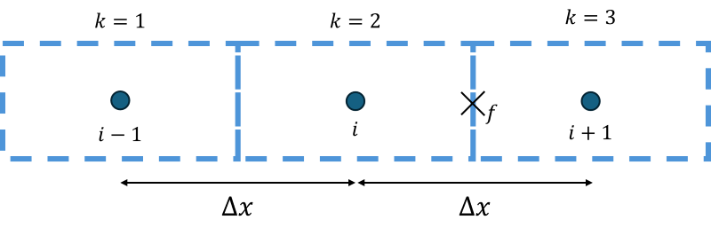
As a reminder, let’s review the following schematic of three cells connected with each other.

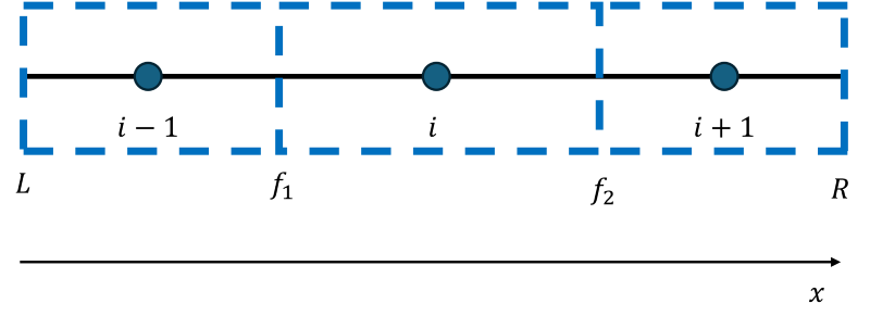
We have values for pressure, velocity, temperature, etc., stored at the cells’ centroids, i.e. at i-1, i, and i+1. Our job now is to provide values at locations f_1 and f_2 based on the values we have at the centroids.

The easiest interpolation scheme we can devise is the central scheme which would give us f_1=(\phi_{i-1}+phi_i)/2 and f_2=(\phi_i+\phi_{i+1})/2, where \phi is just the pressure, velocity, temperature, for example. If life was that easy, I would probably be out of a job and no longer teach CFD, this website would be a joke (or meme), and a monkey could run simulations for us. No, life (and the Navier-Stokes equations, too) is non-linear, and it makes for a fun ride.

In the following sections, we will look at some classical schemes you would likely find in most CFD solvers and then switch to some more advanced schemes that brought CFD from mere higher-order schemes to high-resolution schemes. We’ll discuss them at the end of this section.

First-order upwind scheme

We start with the first-order upwind (FOU) scheme. Similar to the first-order upwind scheme that we saw above for finite differences, the upwind scheme for finite volume methods also involves checking the direction of the flow. Using the notations in the above figures, let’s say we want to approximate the generic variable \phi at the faces f_1 and f_2.

Instead of writing \phi_f_1 and \phi_f_2, we use a more common finite volume notation where we have f_1=i-1/2 and f_2=i+1/2. This, we have \phi_f_1=\phi_{i-1/2} and \phi_f_2=\phi_{i+1/2}.

If we ignore the upwind direction for the moment, we can use the so-called piecewise constant reconstruction to obtain a first-order reconstruction at our faces. For example, we could write \phi_{i-1/2}=\phi_{i-1} and \phi_{i+1/2}=\phi_i. Or, we could write \phi_{i-1/2}=\phi_i and \phi_{i+1/2}=\phi_{i+1}. So which one should we use? Well, similar to the discussion above, when we looked at the upwind scheme in the context of the finite difference method, we have to find the upwind direction.

This is done by checking the local flow velocity, and based on that velocity, we decide which direction to pick. Thus, we can write the first-order accurate upwind scheme for the finite volume method as:

\phi_{i+1/2}^{FOU}=\delta^+\phi_{i+1}+\delta^-\phi_i

For completeness, \phi_{i-1/2} is given as:

\phi_{i-1/2}^{FOU}=\delta^+\phi_{i}+\delta^-\phi_{i-1}

Though, from now on, we will only deal with the face at i+1/2, we can always formulate the same scheme at i-1/2 by shifting the indices i by one to the left, as we saw above.

Similar to the finite difference method, we define \delta^+ and \delta^- as:

\delta^+=\begin{cases}1\quad\quad\quad u_i<0\\0\quad\quad\quad u_i\ge 0\end{cases}

\delta^-=\begin{cases}0\quad\quad\quad u_i<0\\1\quad\quad\quad u_i\ge 0\end{cases}

I have mentioned the piecewise constant reconstruction scheme here, so let’s review that as well for completeness. This scheme is schematically shown below.

With the piecewise constant scheme, we are saying that the values within the cell are constant and do not change. This makes sense; we have a single centroid per cell, and with just one value per cell, we can only really represent a constant state. What we are saying with the piecewise constant reconstruction now is that we can find values at the cell faces by simply copying values from the centroid to the face. If we do so, we see that we get two different values at the cell face, one from the left and one from the right.

Since the piecewise constant scheme does not care about the upwind direction, it doesn’t know which value to take here, so the scheme by itself is not useful. But, we can combine this numerical approximation for the left-sided and right-sided extrapolation with a Riemann solver. The Riemann solver will take both states from the left and the right and consolidate both states into a single value.

If you want, you can think of upwind schemes as the world’s simplest Riemann solver. (Well, upwind schemes are not Riemann solvers, I should be clear about it, but both the upwind scheme and Riemann solvers are trying to find the best possible value at the face through different mechanisms).

Riemann solvers are only applicable to hyperbolic equations, and, for that reason, you will only really find them used for compressible flows (and sometimes, some exotic researchers (like myself, I suppose) use Riemann solvers for incompressible flows as well). I have written a lot more on Riemann solvers in my (free) eBook on how to write your first CFD solver, which may be of interest to you if you want to find out more.

Upwind methods, on the other hand, are more commonly used for incompressible flows. So, depending on the type of flow you are solving, you may want to use one or the other. However, again, these first-order methods are really not that great in terms of accuracy; they both have a lot of numerical dissipation. For that reason, we prefer to use higher-order schemes, which we discuss in the next sections.

Second-order upwind scheme

Similar to the finite difference discussion, we can introduce a second-order accurate version of the upwind method. In some literature, you will also find the acronym SOU (second-order upwind), so if you come across that, this is what it means.

Let us build this second order upwind scheme with some intuition. In the second-order upwind scheme that we discussed in the finite difference context above, we saw that the key to increasing the order is to include additional points in our stencil. So if the first-order upwind method only requires information from cell i in the finite volume context, it stands to reason that for the second-order upwind method, we ought to include information from i+1 or i-1, depending on the upwind direction.

Let’s say we want to find the value of \phi_f_2=\phi_{i+1/2} and the upwind direction is against the x-direction, that is, we want to use \phi_i and \phi_{i-1} in our stencil. I am using the following figure again for the notation in my stencil:

When we looked at the Taylor series expansion in my article on how to discretise the Navier-Stokes equations, I started with the example of wanting to predict the temperature for some time in the future. Let’s assume for a moment that the x-axis above represents time, \phi_i represents the temperature now, and we want to find what the temperature is at some point in the future, i.e. \phi_{i+1/2}.

In the above-linked article, we said the simplest approximation is to say that the temperature at \phi_{i+1/2} is the same as now, i.e. at \phi_{i}. This does look an awful lot like the first-order upwind method, doesn’t it? (Time is always flowing in the same direction; the upwind direction is always against the flow of time in this case).

How did we get a better approximation for the temperature prediction? Well, we said that if we also had information from yesterday, then we could calculate how much the temperature increased or decreased over the last day and use that to correct this first-order approximation of the temperature. Calculating the change in temperature (or, in general, for \phi) and normalising that by the distance over which this change was measured (e..g. one day), provides us with the gradient of temperature (of \phi)

So, to improve our first-order upwind method, we can include the upwind gradient to get a better approximation. This can be written as:

\phi_{i+1/2}=\phi_i+\frac{\phi_i-\phi_{i-1}}{\Delta x}r

We have introduced r here, which is the distance from i to i+1/2. If we have a grid where \Delta x is constant for all cells, then r=\Delta x/2, as the face at i+1/2 is halfway between two centroids or half a cell’s width away. If we have a non-uniform grid spacing, e.g. we are using an unstructured grid with triangles or tetrahedra, then we need to compute r for each cell individually.

In a similar manner, we can also define a forward version for the approximation introduced above for \phi_{i+1/2}. This will use \phi_i and \phi_{i+1} in our stencil. This can be written as:

\phi_{i+1/2}=\phi_{i+1}-\frac{\phi_{i+1}-\phi_{i}}{\Delta x}r

We can now construct our second-order upwind scheme as per the usual approach, that is:

\phi_{i+1/2}^{SOU}=\left[\phi_i+\frac{\phi_i-\phi_{i-1}}{\Delta x}r\right]\delta^-+\left[\phi_{i+1}-\frac{\phi_{i+1}-\phi_{i}}{\Delta x}r\right]\delta^+

Here, we used the same definitions for \delta^+ and \delta^- as before.

Central scheme

The central difference (CD) scheme is pretty straightforward. If we have an equidistant spacing in our mesh, that is, each cell has the same dimension, then we can find a simple approximation for values at cell faces as:

\phi_{i+1/2}^{CD}=\frac{\phi_i+\phi_{i+1}}{2}

This is the same as saying that we are taking an average of neighbouring centroid values to find the value at the cell faces. It only gets slightly more complicated if the spacing is non-uniform, as the following figure shows:

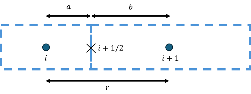
Now we have to weight each cell’s contribution to the value calculated at i+1/2. This can be written as:

\phi_{i+1/2}^{CD}=\frac{b}{r}\phi_{i}+\frac{a}{r}\phi_{i+1}

As the point i+1/2 gets closer to i, a becomes smaller and smaller, while b approaches the value of r. Thus, we weight the contribution at i with b/r, which will get closer and closer to 1 as the face approaches the centroid in i. Thus, the centoid value that is closest to the face should have the largest weight, and this is what the above equation ensures.

For the special case that we have an equidistant spacing again, we have a/r=0.5 and b/r=0.5, i.e. we recovered the simplified version that we started our section on the central scheme with.

We use the central scheme anywhere but the non-linear term. We can use it within the diffusive term, the pressure gradient, and the continuity equation. This is true, at least, for incompressible flows in a non-conservative formulation. For compressible flows, we like to group all of our flow quantities together in a vector form and then use the same scheme for all quantities alike, and we will see that in more detail in the article on incompressible vs. compressible flows.

For completeness, let’s also look at the modified version of the central scheme. We saw in the finite difference section above that we can modify the central differencing scheme to be stable even for convective flows if we supply it with some additional dissipation. We stated that as

\phi_{i+1/2}^{CD}=\frac{\phi_i+\phi_{i+1}}{2}-D_i

Here, we can approximate the dissipation term with the JST scheme, for example, as highlighted above. I wanted to mention this here as it will become important in the next section.

QUICK scheme

The QUICK (Quadratic Upstream Interpolation for Convective Kinematics) scheme uses a polynomial expansion to approximate values at the cell interface. It is nominally third-order accurate, but that may reduce on unstructured grids (for which it is more difficult to implement as well, where some modifications have to be made).

The QUICK scheme outlines an approach that can be extended to any higher order, in theory, making it a general framework. However, it is most commonly presented in the form that I will show below, and most textbooks don’t bother to derive it. But once you understand the derivation, it is actually very easy to derive higher orders yourself.

The QUICK scheme starts with a polynomial description, where we are trying to approximate some quantity \phi_f at the face of the cell. This can be written in compact summation form as:

\phi_{i+1/2}=\sum_{j=1}^n P_j(x)

In theory, we can have as many polynomial coefficients P_j(x) as we want, but the QUICK scheme, where the Q stands for quadratic, only uses three, i.e. n=3, to obtain a quadratic polynomial. I am assuming here that we are only deriving this scheme in one direction (here, the x-direction), hence the polynomial depending on x. The question then becomes what polynomial description we should use for P_j(x).

When Leonard introduced his QUICK scheme in 1979, we already knew about Lagrangian polynomials, which made his job a lot easier. These allow us to calculate the polynomial coefficients of arbitrarily large polynomials. The general formula is given as:

P_j(x)=\phi_j\prod_{\substack{k=1\\k\ne j}}^n\frac{x_f-x_k}{x_j-x_k}=\phi_j\cdot a_j

Here, \phi_j are the values at the various grid points, e.g. \phi_{i-1}, \phi_i, \phi_{i+1}, and so on. So the only thing we have to evaluate is the product, i.e. the a_j coefficient. If we assume that these coefficients are known, for the moment, then our general polynomial description, using the two formulas given above, can be written as:

\phi_{i+1/2}=\phi_{i-1}\cdot a_1+\phi_i\cdot a_2 + \phi_{i+1}\cdot a_3

So, let’s introduce some additional notation, which is done in the figure below:

When we are looping with k from one to n, then we are looping over the three centroids, as shown in the figure above. So k=1 is the location at i-1, k=2 is at location i and k=3 is at location i+1.

For the QUICK scheme, we say that we have two bracketing nodes, that is, both nodes i and i+1 bracket the face value at location i+1/2=f (we could also say f is surrounded by i and i+1). We supplement the stencil now with an upstream node, which we assume to be at i-1, i.e. the flow is coming from the left and is going to the right. Since we introduce upwinding here again, we satisfy the transportiveness criterion for our numerical scheme.

Let’s look at the product again above. We loop here from k=1 to n, which in this case is n=3 as we are considering three centroids. But, if k=j, then we are not including this in our product. j is coming from the summation in the first equation.

Ok, so let’s evaluate the first product a_1. In this case j=1 and so we are only using k=2 and k=3. Keeping in mind the above mapping between k and the cell centroid locations, we get:

a_1 = \prod_{\substack{k=1\\k\ne 1}}^n\frac{x_f-x_k}{x_j-x_k}=\frac{x_f-x_2}{x_1-x_2}\frac{x_f-x_3}{x_1-x_3}=\frac{x_{i+1/2}-x_{i}}{x_{i-1}-x_i}\frac{x_{i+1/2}-x_{i+1}}{x_{i-1}-x_{i+1}}=\frac{\Delta x/2}{(-\Delta x)}\frac{(-\Delta x/2)}{(-2\Delta x)}=-\frac{1}{2}\frac{1}{4}=-\frac{1}{8}

If we have, for example, x_1 - x_2, then we have to translate that into locations i first. This results in x_{i-1}-x_i. We can see that this is just \Delta x from the figure above, but because of the order of the subtraction, it is -\Delta x. Since each term depends on \Delta x, it cancels out, and we can write the coefficient independent of \Delta x.

The other thing to look out for is that the location at the face f is \Delta x/2 away from both location i and i+1, i.e. we are assuming a uniform grid here. If our grid is non-uniform or even unstructured, then we need to evaluate the above product for each cell. If it is equidistant and it stays constant for all cells, then we only need to evaluate it once, as we have done above.

Thus, the first coefficient a_1=-1/8 has been found, and now it is a matter o repeating the produces. For a_2, we have:

a_2 = \prod_{\substack{k=1\\k\ne 2}}^n\frac{x_f-x_k}{x_j-x_k}=\frac{x_f-x_1}{x_2-x_1}\frac{x_f-x_3}{x_2-x_3}=\frac{x_{i+1/2}-x_{i-1}}{x_{i}-x_{i-1}}\frac{x_{i+1/2}-x_{i+1}}{x_{i}-x_{i+1}}=\frac{1.5\Delta x}{\Delta x}\frac{(-\Delta x/2)}{(-\Delta x)}=\frac{3}{2}\frac{1}{2}=\frac{3}{4}=\frac{6}{8}

In this case, j=2 and so we have k=1 and k=3. Then we figure out the distances again and arrive at the second coefficient, which in this case is a_2=6/8.

For a_3, we have j=1 and so k=1 and k=2, which results in:

a_3 = \prod_{\substack{k=1\\k\ne 3}}^n\frac{x_f-x_k}{x_j-x_k}=\frac{x_f-x_1}{x_3-x_1}\frac{x_f-x_2}{x_3-x_2}=\frac{x_{i+1/2}-x_{i-1}}{x_{i+1}-x_{i-1}}\frac{x_{i+1/2}-x_{i}}{x_{i+1}-x_{i}}=\frac{1.5\Delta x}{2\Delta x}\frac{\Delta x/2}{\Delta x}=\frac{3}{4}\frac{1}{2}=\frac{3}{8}

Thus, we have obtained a_3=3/8. With these coefficients found, we can insert them into our first equation and obtain the following approximation for \phi_f:

\phi_{i+1/2}=-\frac{1}{8}\phi_{i-1}+\frac{6}{8}\phi_i + \frac{3}{8}\phi_{i+1}

Let’s rewrite this equation in a slightly different form. Let’s decompose the second and third terms into two separate components, as shown in the following:

\phi_{i+1/2}=-\frac{1}{8}\phi_{i-1}+\left(\frac{4}{8}\phi_i + \frac{2}{8}\phi_i\right) + \left(\frac{4}{8}\phi_{i+1}-\frac{1}{4}\phi_{i+1}\right)

Now, we can write this in a different form:

\phi_{i+1/2}=\frac{\phi_i+\phi_{i+1}}{2}-\frac{\phi_{i-1}-2\phi_i+\phi_{i+1}}{8}

This is just the central scheme with some additional corrections. Does this remind you of something? How about the central scheme with artificial dissipation?

\phi_{i+1/2}=\frac{\phi_i+\phi_{i+1}}{2}-D_i

While the JST scheme puts some user-defined dissipation here, the QUICK scheme simply provides a correction here (to be precise, a quadratic correction) to the linear approximation of the central scheme, and this makes the scheme stable.

We saw that we needed to include an upwind node at the beginning of the derivation, and I just assumed that to be at i-1. But what if the flow is going the other direction? Then my bracketing nodes would still be i and i+1, but this time, the upwind node would be at i+2!

We can carry out the evaluation of the polynomial coefficients in the same manner for this stencil, and the approximation for \phi_f would result in

\phi_{i+1/2}=\frac{3}{8}\phi_i+\frac{6}{8}\phi_{i+1}-\frac{1}{8}\phi_{i+2}

They have the same coefficients, just differently arranged. Now, if we want to construct a general scheme where the flow can either come from the left or right, we introduce our \delta^+ and \delta^- coefficient as we did in the upwind scheme and obtain

\phi_{i+1/2}^{QUICK}=\left[-\frac{1}{8}\phi_{i-1}+\frac{6}{8}\phi_i + \frac{3}{8}\phi_{i+1}\right]\delta^-+\left[\frac{3}{8}\phi_i+\frac{6}{8}\phi_{i+1}-\frac{1}{8}\phi_{i+2}\right]\delta^+

MUSCL scheme

The Monotonic Upstream-centered Scheme for Conservation Laws, also known by its street name MUSCL, is an attempt to recover higher-order accuracy for flows with strong non-linear effects such as shock waves and, in general, discontinuous signals. Thus, it is very much a scheme for highly compressible flows, but it can be used for incompressible flows with some modifications as well. Let’s look at the scheme in detail.

To understand the motivation for the MUSCL scheme, we have to understand a fundamental limitation that existed up until the 1970s, i.e. up until Van Leer introduced his MUSCL scheme over a series of 5 papers between 1973-1979 in two different journals (why write only one paper when you can spread your knowledge over five paper, and have them published several years apart? I shall, from now on, publish all my papers with sequels in mind to make me look really research active …)

In 1954, Godunov introduced and proved the following statement, which has become known as the Godunov theorem:

Linear numerical schemes for solving partial differential equations (PDE’s), having the property of not generating new extrema (monotone scheme), can be at most first-order accurate.

What this means in plain English is that only first-order schemes, such as the first-order upwind method, can be used without introducing new min and max values. Take the following simulation, for example, where the advection equation u_t+au_x=0 is solved with an initial box profile. The solution for the first-order upwind scheme is shown on the left, while a second-order scheme is shown on the right.

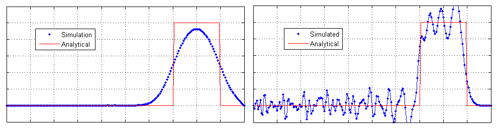
Let’s say that the box itself has a y value of 1, i.e. the largest (max) value we would expect is 1. Where we have no profile, i.e. just a flat line, the y value is 0; thus, the lowest (min) value is 0. The first-order accurate scheme is between these two min/max values. Or, using Godunov’s terminology, we do not introduce any new extrema.

Compare that with the second-order scheme on the right. Here, the interpolation results in values that are above the max value of 1 and below the min value of 0. Thus, the second-order scheme does introduce new extrema. If this profile represented the density, for example, we would run risk of computing a negative density, and this would result in all sorts of numerical, and physical. problems.

Thus, Godunov found and proved that in order to retain interpolated values that do not produce new extrema, we need to use first-order schemes. But, first-order schemes are really dissipative, more so than we like, as I have already alluded to a few times (talking about the first-order upwind method).

For smooth signals, i.e. those where we don’t have any shock waves or other discontinuities (e.g. interfaces), this isn’t too much of a problem. We would still like higher-order accuracy if we can, but we can live with first-order schemes if we have to. For compressible flows, though, first-order schemes are too dissipative, and a solution was needed.

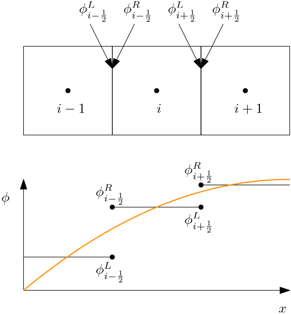
Van Leer went on to solve this issue, starting with his first paper in 1973 and then publishing his solution all the way into 1979. The main idea of the MUSCL scheme is as follows: Take a first order accurate approximation for the value at the cell face, without knowing the upwind direction, this could come from either side of the face. This scheme is known as the piecewise constant reconstruction and given as:

\phi_{i+1/2}^L=\phi_i\quad\quad\quad\phi_{i+1/2}^R=\phi_{i+1}

To understand this notation, let’s review the following figure:

Here we can see that \phi_{i+1/2} can have two possible values, either using a left-sided or right-sided interpolation. If we approach the face from its left face, then we are in cell i and so \phi_{i+1/2}^L=\phi_i. Equally, if we approach the cell to its right face, we get \phi_{i+1/2}^R=\phi_{i+1} as the interpolation. From the diagram below the cells, where the orange line represents the continuous solution we have, we see that both of these approximations simply take the value at their centroid and copy that to the cell’s face.

This means that \phi_{i+1/2}^L\ne\phi_{i+1/2}^R. We can now introduce our upwinding mechanism again, using \delta^+ and \delta^-, and this provides us with the first-order upwind scheme we looked at above. Or, we could solve the Riemann problem, which is what Godunov and others have done. Solving the Riemann problem is only applicable to hyperbolic equations, though, and thus, it is typically only performed for compressible flows. Incompressible flows would use upwinding here.

OK, so now we have the starting point for the MUSCL scheme. We could now improve upon this first-order reconstruction, i.e. the piecewise constant reconstruction, and introduce a piecewise linear reconstruction. This would be second-order accurate. For an equidistant grid, this can be written as:

\phi_{i+1/2}^L=\phi_i+0.5(\phi_{i+1}-\phi_i)\quad\quad\quad\phi_{i+1/2}^R=\phi_{i+1}-0.5(\phi_{i+2}-\phi_{i+1})

Here, we take the value at the cell centroid i for the left-sided interpolation and i+1 for the right-sided interpolation and correct this constant value. For example, referring to the figure above, we can see that 0.5(\phi_{i+1}-\phi_i) would provide us with a more accurate prediction at \phi_{i+1/2}, if we add that to the value of \phi_i. This is what this correction is doing, essentially, i.e. predicting a better approximation for values at the face connecting two cells.

But we saw previously that this type of central stencil essentially violates the transportiveness property, and the result was shown above in the comparison between first-order and second-order schemes. So, the scheme presented above is not yet finished.

In order to ensure that no new extrema were introduced, van Leer introduced a limiter \Psi(r), which he inserted into the scheme as:

\phi_{i+1/2}^L=\phi_i+0.5\Psi(r_i)(\phi_{i+1}-\phi_i)\quad\quad\quad\phi_{i+1/2}^R=\phi_{i+1}-0.5\Psi(r_{i+1})(\phi_{i+2}-\phi_{i+1})

The function of the limiter is two-fold. If the signal is smooth and no discontinuity is present, then the limiter should be switched off, i.e. produce a value of 1, so that it does not interfere with the solution. If \Psi(r)=1, then it does not influence the interpolation, and we recover the original second-order accurate description.

If the flow does have discontinuities, though, then the limiter should detect these, and in regions of discontinuities, it should produce a value of \Psi(r)=0. This means that the second term in our numerical approximation formula above is zero, and we recover the piecewise constant reconstruction. We know that this piecewise constant reconstruction will not introduce new extrema, thanks to Godunov’s theorem, and as a result, we will get an overall better accuracy in our simulation.

The original MUSCL scheme was introduced with the formula given below, which was also referred to as the \kappa-scheme in some references. For the left-sided interpolation, we obtain:

\phi_{i+1/2}^L=\phi_i+\frac{1}{4}\Psi(r_i)\left[(1-\kappa)(\phi_{i}-\phi_{i-1})+(1+\kappa)(\phi_{i+1}-\phi_{i})\right]

And, for the right-sided interpolation, we obtain:

\phi_{i+1/2}^R=\phi_{i+1}-\frac{1}{4}\Psi(r_{i+1})\left[(1+\kappa)(\phi_{i+1}-\phi_{i})+(1-\kappa)(\phi_{i+2}-\phi_{i+1})\right]

Here, we have a new parameter \kappa, and depending on its value, we recover different versions of this scheme. In general, \kappa can be set between -1 and +1, though the following values are generally used:

• \kappa=-1: This results in the second-order upwind scheme
• \kappa=0: This results in the second-order Fromm scheme (less used these days)
• \kappa=1/3: This results in the third-order MUSCL approximation. Don’t tell van Leer that this is only second-order accurate, or he may go ballistic …

To understand the full MUSCL scheme, we need to look at the limiter \Psi(r) and its argument r, which we will do in the next section.

Flux limiters

I’ve spent quite some time trying to find a good angle to talk about flux limiters, and I realised that giving them a proper introduction would require an entire article on its own. Whatever depth I would be able to cover on flux limiters in this already excessively long article would do it an injustice. So, here’s the deal: I’ll introduce them more broadly in this section and then follow up with a blog post on the proper derivation of flux limiters. Deal? (Well, this is rhetorical; I can’t hear you scream at your screen … Let’s continue, then.)

There are two parts to flux limiters that we need to understand. Smoothness and total variation. Total variation is just the sum of subsequent entries in a vector containing our flow solution for \phi. This can be expressed as

TV(\phi)=\sum_{i=1}^{n-1}(\phi_{i+1}-\phi_i)

In the section above on the MUSCL scheme, we looked at two simulation results for the box profile. One was smooth, and the other had quite a few oscillations. If we generate these oscillations, they will only grow over time, and thus, the total variation will increase with time. We can use this property to construct flux limiters that will keep the total variation the same (or reduce it) over time. If this is the case, then we have a total variation diminishing (TVD) scheme, and we have removed spurious oscillations from our simulations.

The smoothness, on the other hand, is measured as the ratio of two subsequent gradients. For example, we could express the gradients at two adjacent grid points i and i+1 as:

\frac{\partial \phi_i}{\partial x}\approx\frac{\phi_i-\phi_{i-1}}{\Delta x}\quad\quad\quad\frac{\partial \phi_{i+1}}{\partial x}\approx\frac{\phi_{i+1}-\phi_{i}}{\Delta x}

The ratio of the two gradients is then computed as:

r=\frac{\frac{\phi_i-\phi_{i-1}}{\Delta x}}{\frac{\phi_{i+1}-\phi_{i}}{\Delta x}}=\frac{\phi_i-\phi_{i-1}}{\phi_{i+1}-\phi_{i}}\frac{\Delta x}{\Delta x}=\frac{\phi_i-\phi_{i-1}}{\phi_{i+1}-\phi_{i}}

r is known as the smoothness indicator. Let’s investigate a few possible cases for how r can look. For that, let’s investigate the following figure, which shows a few possible solutions that are either smooth or discontinuous:

For the first case on the left, we have a relatively smooth profile of r, and we can compute it using the values given at the top right corner of the plot. This then results in

r=\frac{\phi_i-\phi_{i-1}}{\phi_{i+1}-\phi_{i}}=\frac{1.25-1.5}{1.0-1.25}=\frac{-0.25}{-0.25}=1

If we compare that with the actual gradients (assuming \Delta x=1):

\frac{\partial \phi_i}{\partial x}\approx\frac{\phi_i-\phi_{i-1}}{\Delta x}=\frac{1.25-1.5}{1}=-0.25\\
\frac{\partial \phi_{i+1}}{\partial x}\approx\frac{\phi_{i+1}-\phi_{i}}{\Delta x}=\frac{1.0-1.25}{1}=-0.25

We see that these gradients are indeed the same values used in the smoothness indicator r. Furthermore, we can see that for smooth regions, in which there is no sudden change in gradients, the smoothness indicator will return a value of near 1, or 1 exactly if adjacent gradients are exactly the same.

Let’s review the second case in the figure above. Here we have a sudden drop in \phi, which could, for example, represent a shock wave (arguably a not so well resolved shock wave!). If we perform the same calculation here, then we get a smoothness indicator of r=8. Thus, near discontinuities, the smoothness indicator will increase and take on values far away from 1.

Thus, the smoothness indicator does provide an effective measure for separating smooth regions from discontinuous profiles. What about the last case, i.e. the plot on the right? We have a constant profile, no change, and the gradients are zero, so what is its smoothness? We would expect a value of 1, but if we insert the actual values, we get

r=\frac{1-1}{1-1}=\frac{0}{0}=trouble

In regions where the flow is giving no gradients, the concept of smoothness breaks down. We have to modify the smoothness indicator in the region, and we do that by adding a small number to the denominator (typically 10^{-10}\le\varepsilon\le 10^{-6}). If we don’t do this, we are in trouble.

Say you want to use the smoothness indicator for limiters in your simulation; then, at the beginning of your simulation, you may initialise the flow with uniform values in the entire domain, giving you NaN (not a number) for your smoothness indicator everywhere. This will propagate in your calculations, and your simulation will crash within the first time step or iteration. Thus, we want to introduce the above modification, which results in

r=\frac{\phi_i-\phi_{i-1}}{\phi_{i+1}-\phi_{i}+\varepsilon}

Thus, if there are no gradients, r\rightarrow\infty. As we will see in a second, this isn’t a problem, though.

Now that we have a concept of smoothness, let’s review the limiter \Psi(r) itself. Based on the smoothness indicator, we want to transform. This is the part where I mentioned that we need an entire article on its own to derive the required stability limits. So, for now, we will accept them as they are and then return back to them in due time.

In 1984, Sweby derived the required limits for \Psi(r) to provide a second-order accurate reconstruction. This can be graphically shown in a \Psi(r)-r diagram, which we also call the Sweby diagram. This is given below:

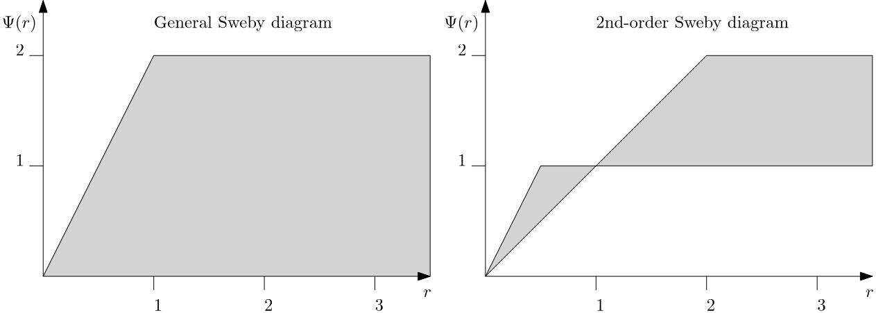
The shaded gray area provides a region where reconstructed schemes will retain second-order accuracy. So, let’s step back and discuss what that means. On the x-axis, we see the smoothness indicator r. We saw that for large values of it, we enter regions of stronger differences in gradients. For discontinuities, we get very large values of r. If we now construct a limiter \Psi(r) that will produce values regardless of r that always fall within the gray-shaded area, then we have a second-order scheme.

This means that we have just gone beyond Godunov’s theorem and shown that we can construct schemes that do not introduce new extrema while being second-order. This was a massive achievement in the field of CFD and one that we still greatly benefit from today. The introduction of limiters has greatly advanced the field of CFD.

I should mention here that I have only shown the Sweby diagram here for values of r up to about 3, but it does extend to infinity, i.e. regardless of the value of r, if r\ge 2 and 1\le\Psi(r)\le 2, we have a stable and second-order accurate scheme.

A few popular limiters are given below:

• van Leer: \Psi(r)=(r+|r|)/(1+|r|)
• van Albada: \Psi(r)=(r^2 +r)/(r^2 +1)
• minmod: \Psi(r)=\max[0,\min(1,r)]
• superbee: \Psi(r)=\max[0, \min(2r, 1), \min(r, 2)]

There are just as many limiters as turbulence models, and you can even develop your own limiter. As you can see, it isn’t that difficult; as long as you are within the gray shaded area, you are guaranteed to get a second-order accurate reconstruction. And since this is a very straightforward process, many people published their own limiters to get name recognition, I suppose.

The examples I have picked above are on purpose; you can see that the first two limiters are differentiable, while the last two are not (in other words, the first two limiters will provide a smooth profile, while the last two limiters have discontinuous jumps in their limiter function). This can affect your convergence rate if you are operating near one of these discontinuities in your limiter.

This doesn’t mean that differentiable limiters are always to be preferred over non-differentiable limiters; it is very much a case of checking which limiter works best for your application and then using it. But you may need to use a different limiter for your next project, so testing is important here.

Wikipedia has a good overview of different limiters, not just their equation, but also a visual representation of each limiter, i.e. how they fit into the Sweby diagram, which I have blatantly ripped off from them for your viewing pleasure. See below:

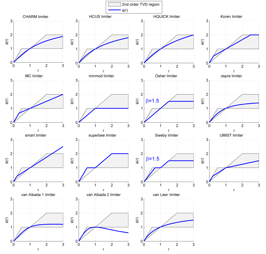
You see that not all schemes are within the shaded gray area. This just means that they aren’t second-order accurate and, potentially, may not work well with high values of r, i.e. in regions of strong shocks. Again, testing is important, and a good portion of belief and religion into which limiter to worship will also go a long way.

My favourite limiter, you ask? I’m glad you did (I thought you would never ask!). Well, there are so many fantastic limiters to choose from, but my favourite must be the Tom limiter that I literally just came up with. This is given as:

\Psi^{TOM}(r)=\begin{cases}
r &r<1\\
1+(r-1)^2 &1\le r<2\\
\frac{3}{2}+\frac{1}{2}\cos[\pi (r-2)]\quad\quad &r\ge 2
\end{cases}

If we plot it, we get this beauty:

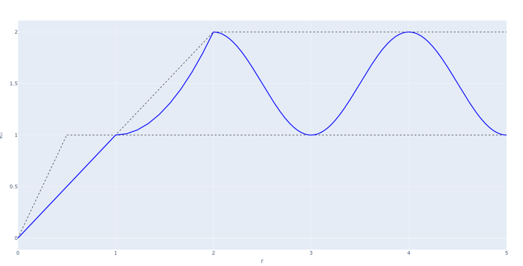
I haven’t tested it, but I don’t need to, either; it’ll work! And no, this isn’t taking the piss (perhaps just a little), I’m using a smooth cosine function here which is differentiable for non smooth regions to give you smooth convergence for your strong discontinuities. My question to you is, can you come up with a limiter that is even more ridiculous?

Well, jokes aside, limiters are really powerful, as we have seen, as they allow us to recover second-order accuracy and extend Godunov’s theorem. But there is just one problem. Let’s look at the definition of the MUSCL scheme again (we’ll use the second-order version, but the general \kappa scheme would work as well here):

\phi_{i+1/2}^L=\phi_i+0.5\Psi(r_i)(\phi_{i+1}-\phi_i)\quad\quad\quad\phi_{i+1/2}^R=\phi_{i+1}-0.5\Psi(r_{i+1})(\phi_{i+2}-\phi_{i+1})

We have seen that it is possible for the smoothness indicator to take on large values. We saw that this was the case for a discontinuity, where we go from a large to a low value. If we repeat this process, but now go from a low to a large value across the discontinuity, the value for r will approach zero. In this case, we have \Psi(r=0)=0, and this forces the scheme to become locally first-order, i.e. our reconstruction scheme with \Psi(r)=0 reduces to:

\phi_{i+1/2}^L=\phi_i\quad\quad\quad\phi_{i+1/2}^R=\phi_{i+1}

So, in areas of strong discontinuities, we switch to a first-order description while we go back to second-order in smooth regions. This is one limitation we have to accept with limiters, but we know from experience that this isn’t a practical limitation. Overall, results with limiters are much better than without.

WENO scheme

OK, so if flux limiters deserve their own article as they are a bit more complicated, then WENO schemes deserve their entire own series as they are rather complex and multi-faceted. They provide enough ammunition to fill an entire book on their own. So, as with flux limiters, we’ll concentrate here on the essentials, trying to get an understanding of what WENO schemes are and how to implement them, but I’ll have to take a shortcut on the mathematics. There are quite a few things I have to gloss over, but that shouldn’t stop us from getting an understanding of what WENO schemes are.

If we want to understand WENO schemes, we first have to start with ENO schemes. ENO stands for essentially non-oscillatory, and the idea behind this scheme is to approximate a value \phi_{i+1/2} by a polynomial. Well, this is essentially what we did with the QUICK scheme above, so what’s the difference?

When we used the QUICK scheme, we only used a single polynomial to construct the value at \phi_{i+1/2}. In ENO schemes, we construct more than one polynomial to approximate \phi_{i+1/2}, and then we check which gives us the smoothest solution.

For the MUSCL scheme, we saw that we can introduce a limiter and suppress oscillations based on some smoothness indicator. In ENO schemes, we simply construct more polynomials and then hope that at least one of them is smooth. Whichever is smoothest will be selected for computing \phi_{i+1/2}.

To make this more concrete. For the QUICK scheme we used a stencil that included points at S(i-1,\, i,\, i+1) to compute \phi_{i+1/2}, assuming here that the upwind direction is in the negative x-direction (and thus the upwind node at i-1).

For ENO schemes, we may construct three polynomials with stencils S_1 (i-2,\, i-1,\, i), S_2 (i-1,\, i,\, i+1), and S_3 (i,\, i+1,\, i+2). We then check the smoothness of each polynomial, and then either select S_1, S_2, or S_3 depending on the smoothness indicator, which is differently defined for ENO and WENO schemes comared to what we saw previously in the MUSCL scheme and flux limiters.

WENO schemes take the idea of ENO schemes one step further by not simply selecting the smoothest polynomial reconstruction but instead combining all of them in a weighted fashion. By doing this, we increase the size of the stencil and, thus, the order of the overall approximation.

WENO schemes have become the gold standard for approximating discontinuities in compressible flows, and they produce outstanding results on even coarse grids. So now that I hopefully made you crave for more, let’s quench that WENO thirst of yours and look at how we can actually implement that.

We start by constructing our polynomials. We first have to decide how many polynomials we want to use. A common choice is to use three polynomials with a 3-point stencil, similar to the example that I provided above. This will result in a 5^{th} order accurate WENO reconstruction for \phi_{i+1/2}, at least in smooth regions. Our three polynomials can be defined as:

\phi^{(1)}_{i+1/2} = \frac{1}{3}\phi_{i-2}-\frac{7}{6}\phi_{i-1}+\frac{11}{6}\phi_{i}\\[1em]
\phi^{(2)}_{i+1/2} = -\frac{1}{6}\phi_{i-1}+\frac{5}{6}\phi_{i}+\frac{1}{3}\phi_{i+1}\\[1em]
\phi^{(3)}_{i+1/2} = \frac{1}{3}\phi_{i}+\frac{5}{6}\phi_{i+1}-\frac{1}{6}\phi_{i+2}

Now, we need to calculate the smoothness indicator for each stencil. This means we look at the values of \phi that are used in each stencil. Thus, we do not look at each polynomial reconstruction itself, but rather the values that are used for creating these polynomial reconstructions in the first place. Then, if there are any large jumps in values of \phi, we will know that the underlying polynomial reconstruction is based on non-smooth input data, and thus, we would obtain a large value for the smoothness indicator itself.

A large value in the smoothness indicator, as we will see shortly, would then effectively suppress this polynomial by giving it a low weight. So, let’s compute these smoothness indicators. Note, in the WENO literature, smoothness indicators are expressed by the letter \beta (or sometimes IS) instead of r, so I will follow the same nomenclature here. \beta can be calculated for each stencil as:

\beta^{(1)}=\frac{13}{12}(\phi_{i-2}-2\phi_{i-1}+\phi_{i})^2+\frac{1}{4}(\phi_{i-2}-4\phi_{i-1}+3\phi_{i})^2\\[1em]
\beta^{(2)}=\frac{13}{12}(\phi_{i-1}-2\phi_{i}+\phi_{i+1})^2+\frac{1}{4}(\phi_{i-1}-\phi_{i+1})^2\\[1em]
\beta^{(3)}=\frac{13}{12}(\phi_{i}-2\phi_{i+1}+\phi_{i+2})^2+\frac{1}{4}(3\phi_{i}-4\phi_{i+1}+\phi_{i+2})^2

Now that we know what the smoothness indicators are, we can compute the weights that we need to compute a weighted sum of all polynomials. For that, we first define a set of linear weights as:

\gamma^{(1)}=\frac{1}{10}\quad\quad\quad\quad\gamma^{(2)}=\frac{3}{5}\quad\quad\quad\quad\gamma^{(3)}=\frac{3}{10}

Now we can combine these linear weights with the smoothness indicator as:

\alpha^{(1)}=\frac{\gamma^{(1)}}{(\beta^{(1)}+\varepsilon)^2}\\[1em]
\alpha^{(2)}=\frac{\gamma^{(2)}}{(\beta^{(2)}+\varepsilon)^2}\\[1em]
\alpha^{(3)}=\frac{\gamma^{(3)}}{(\beta^{(3)}+\varepsilon)^2}

Finally, we want to normalise our weights so that the sum of all of them is equal to one. This can be achieved with the following equations:

w^{(1)}=\frac{\alpha^{(1)}}{\alpha^{(1)}+\alpha^{(2)}+\alpha^{(3)}}\\[1em]
w^{(2)}=\frac{\alpha^{(2)}}{\alpha^{(1)}+\alpha^{(2)}+\alpha^{(3)}}\\[1em]
w^{(3)}=\frac{\alpha^{(3)}}{\alpha^{(1)}+\alpha^{(2)}+\alpha^{(3)}}

Now that we have obtained our final weights, we can construct our weighted polynomial interpolation, which is given by the following equation:

\phi_{i+1/2}=w^{(1)}\phi_{i+1/2}^{(1)}+w^{(2)}\phi_{i+1/2}^{(2)}+w^{(3)}\phi_{i+1/2}^{(3)}

This provides us with the fifth-order WENO reconstruction. Unlike the MUSCL scheme, which provided us with a left-sided or right-sided interpolation, i.e. \phi_{i+1/2}^L and \phi_{i+1/2}^R, the WENO scheme provides us with the interpolated value at the face directly.

It is possible to extend the above procedure to obtain left-sided and right-sided interpolations again, but this is not without complications. A good reference is Chapter 10 in the book Relativistic Hydrodynamics for a general introduction or Procedure 2.6 to Procedure 2.10 in ENO and WENO Schemes for Hyperbolic Conservation Laws. This reference is more complete (and freely available) but will require some time to read. Instead of \phi_{i+1/2}^L and \phi_{i+1/2}^R, the second reference uses \hat{f}_{i+1/2}^- and \hat{f}_{i+1/2}^+ instead (i.e. the interpolated fluxes, not primitive variables).

With a left-sided and right-sided interpolation available again, we can include the Riemann problem for an even better approximation, though you will see in the second reference that the splitting into left-sided and right-sided interpolation may already include a Riemann solver (e.g. the Roe Riemann solver).

Finally, let’s investigate what happens near a discontinuity. Here, we would obtain large values for \beta for stencils that have a discontinuous signal. Thus, our weights \alpha would become small, and the polynomial constructed on the non-smooth stencil would receive little weight in the final reconstruction. In the worst-case scenario, only one stencil is smooth, and the order of reconstruction reduces locally to the order of the polynomial.

This isn’t necessarily a problem, as WENO schemes provide a smooth transition at discontinuities, even at lower order reconstructions, avoiding oscillations altogether. This is why WENO schemes have become the norm for high-resolution methods for compressible flows, at least in research codes. Commercial solvers do not go anywhere near WENO schemes, as their implementation on an unstructured grid is possible but complicated. While this can be achieved, the computational cost is vastly higher than a simple MUSCL scheme with a single polynomial reconstruction.

Thus, you will likely find MUSCL schemes to be used more frequently in combination with limiters, but a lot of work has happened in the WENO literature over the past decades, so don’t be surprised to see them featured more frequently in CFD solvers.

Numerical schemes for time integrations

In this section, I also want to touch upon common numerical schemes you can use for integrating equations in time. In general, we will have a time derivative of the form partial\phi/\partial t, and we have different choices available for discretising this term.

The good news is that all the work we have done with the Taylor series and the discretisation of finite difference equations can be carried over into the discretisation of the time derivative again. Furthermore, since the time derivative is linear, discretising this term becomes straightforward again. So, in this section, we will review some common choices for discretising our equations in time. Let’s get straight into it.

Euler time integration

This is the most straightforward time integration there is. Whenever you start implementing a new solver, you want to start with this scheme as it is so easy to implement, i.e. it is very difficult to get wrong. The first-order Euler time integration is given as:

\frac{\partial \phi}{\partial t}\approx\frac{\phi^{n+1}-\phi^n}{\Delta t}

This is just a forward difference in the classical Taylor series and finite difference method sense. There is no need for upwinding here, time usually only marches in one direction (i.e. forward), but if you know how to reverse the direction of time and become younger rather than older, let me know! (in return, I show you how to apply a backward difference in time then, I think this is a fair deal …)

This type of time integration is, well, straightforward, but similar to first-order methods we saw before, it is dissipative in time. Most of the modelling error will come from the spatial (non-linear) gradients, so the error we are making here with a first-order Euler in time is not that much of a problem, but if you are investigating some phenomena in time, like turbulence, you likely want to use a higher-order scheme here as well.

Second-order backward

So if you want to get higher-order, well, then the second-order backward scheme is a good starting point. Again, this is a very simple scheme, but it can achieve better accuracy compared to the first-order Euler scheme. It is given as:

\frac{\partial\phi}{\partial t}\approx\frac{3\phi^{n+1}-4\phi^n+\phi^{n-1}}{2\Delta t}

Looks familiar? Yes, this is just the second-order backward approximation we saw in the finite difference method when we looked at second-order upwind approximations. The same Taylor series approach for finding this backward approximation can be used here again to arrive at the results shown above, though in this case, we need a Taylor series for t-\Delta t and t-2\Delta t.

You see, all of that work on the finite difference method using Taylor series isn’t lost on us, even if we want to use the finite volume method exclusively.

The first-order Euler and the second-order backward approximation are good starting points for discretising your flow and likely the time integration schemes you’ll be using in any commercial and even open-source CFD solver. But we can do better than that. Next, I want to look at time integration techniques originally introduced for ordinary differential equations, but these have shown great properties for CFD applications and thus are commonly used, especially if you need a good accuracy in time.

Runge-Kutta type methods

Runge-Kutta type methods are a bit of magic. They can be expensive to use, but they have been tweaked, improved, and optimised for CFD applications over the years that they have become really useful for solving unsteady flows.

The main idea behind the Runge-Kutta method is that we want to find an approximation to the time derivative through a number of stages. Within each stage, we compute an updated solution based on the previous stage and at the end, we sum all approximations together to get a weighted approximation, that usually is very close to the analytic value. Let’s look at an example to see how this works.

The following figure shows this procedure, where we use four stages to approximate the function shown in blue.

First, we start by finding the slope at t_0. This is shown by k_1. We use this slope to go up until t_0+h/2=t_0+\Delta t/2, which gives us the value y_0 +hk_1/2=y_0+\Delta t k_1/2. We can see that the function we are trying to approximate (in blue) has a different slope here, and so when we repeat this process to obtain k_2, we get a better intermediate slope prediction. We repeat this process to get y_0+hk_2/2=y_0+\Delta tk_2/2, i.e. we are trying to iteratively improve our slope prediction. The last predicted slope is at y_0+hk_3=y_0+\Delta t k_3.

Now all that we have to do is to computed a weighted sum of all of these slopes (k_1 -- k_4), which gives us the point shown in green, i.e. (t_1,y_1). As we can see, this value is quite close to the blue line itself. Compare that to the slope k_1, which is essentially our first-order Euler scheme. k_1 would intersect the line t_0+h=t_0+\Delta t at a much lower point on the y-axis compared to the result we obtained with the Runge-Kutta method here.

This is one of the reasons we like to use it for CFD applications, i.e. it is very accurate. However, it should also be stated here that Runge-Kutta methods can be very slow. While we only need one pass to compute the first-order Euler or even second-order backward scheme to obtain our time derivative approximation, in the Runge-Kutta method, we need to compute the time derivative as many times as we have stages. In our example above, we need to compute the time derivative 4 times, and this will slow down your computation significantly.

However, the number of stages typically directly correlates with the order of the time integration scheme. So for example, using 4 stages as we have done above, results in a fourth order Runge-Kutta time integrations scheme. This holds true for Runge Kutta methods up to fourth order (and thus 4 stages), if certain conditions are met, but for fifth-order methods and above, we typically need more stages than the order of the scheme.

In the next section, I want to show you how we can represent Runge-Kutta methods in a compact notation, and then we look at how we can use that compact notation to derive the actual time integration schemes we can implement into our CFD solver.

The general Runge-Kutta method

Typically, Runge-Kutta methods are represented with a so-called Butcher tableau. The general form is given below

\begin{array}{c|cccc}
c_1 & a_{1,1} & a_{1,2} & \dots & a_{1,nCol}  \\
c_2 & a_{2,1} & \ddots & & \vdots \\
\vdots & \vdots & & \ddots & \vdots \\
c_{nRow} & c_{nRow,1} & c_{nRow,2} & \dots & c_{nRow,nCol} \\
\hline \\
 & b_1 & b_2 & \dots & b_{nCol}
\end{array}

OK, so what’s going on here? Typically, this is what you will find when looking up the Runge-Kutta method. I always found the notation confusing, especially when I wanted to bring the Butcher tableau into a form that I can actually implement into code, so let me go over this step in greater detail.

First, there are two conditions that we want to satisfy. The first is that all values of b, when summed up, give a value of one, i.e.

\sum_{i=1}^{nCol}b_i=1

This condition ensures that the Runge-Kutta method is consistent. We will use the values of b later to weigh the different stages. We saw in the WENO section that we also needed to weigh the different polynomials and use weights that sum up to one, otherwise we would be scaling our approximation either up or down.

The second condition, which is not necessarily required but typically enforced to ensure we get the highest-order possible for the number of stages we are using, is that for each row in the butcher tableau, all coefficients of a, when summed up, give the value of c in the same row. This can be expressed as:

c_k=\sum_{i=1}^{nCol}a_{ki}

OK, so with the definitions out of the way, let us now derive the numerical schemes we can use for the time integration. We start with an example, the fourth-order Runge-Kutta scheme we have looked at above in a schematical manner.

Step 1: Define the Butcher tableau

The Butcher tableau for the fourth-order Runge Kutta method can be written as:

\begin{array}{c|cccc}
0 &  0 & 0 & 0 & 0  \\[0.5em]
\frac{1}{2} & \frac{1}{2} & 0 & 0 & 0 \\[0.5em]
\frac{1}{2} & 0 & \frac{1}{2} & 0 & 0 \\[0.5em]
1 & 0 & 0 & 1 & 0 \\
\hline\\[-0.7em]
& \frac{1}{6} & \frac{2}{6} & \frac{2}{6} & \frac{1}{6}
\end{array}

Step 2: Derive equations for each stage

In our case, we see that we have 4 rows in the Butcher tableau (above the horizontal line), which means that we have 4 stages. We ignore the last row for now; this will become important in the next step. The general equation for deriving a single stage s in the Runge-Kutta method is given as

k_s=f\left(t_n+c_s h, y_n+h\sum_{i=1}^{nCol}a_{s,i}k_{i}\right)

Here, n is the current time level (and our goal is to advance to the next time level n+1 using the Runge-Kutta method). This is the notation you will generally find in the Runge-Kutta method, but let’s translate that into something that looks more familiar with standard CFD notation, then we get:

\mathbf{U}^{(s)}=f\left(t_n+c_s \Delta t, \mathbf{U}^{n}+\Delta t\sum_{i=1}^{nCol}a_{s,i}RHS\left(\mathbf{U}^{(i)}\right)\right)

Here, we have \mathbf{U} as the velocity vector, and a subscript of n just denotes that it is at time level n. h has now become the time step \Delta t, and with each stage, our goal is to calculate an updated velocity vector at stage s, i.e. \mathbf{U}^{(s)}.

A larger striking change is the last argument, which changed from k to RHS(\mathbf{U}). Let’s remind ourselves what we want to achieve here. We typically want to solve some variation of the Navier-Stokes equations, i.e.

\frac{\partial \mathbf{U}}{\partial t}+(\mathbf{U}\cdot\nabla)\mathbf{U}=-\frac{1}{\rho}\nabla p +\nu\nabla^2\mathbf{U}

Let’s separate the time derivative from the rest of this equation, i.e. everything except the time derivative has to go on the right-hand side (RHS):

\frac{\partial \mathbf{U}}{\partial t}=-(\mathbf{U}\cdot\nabla)\mathbf{U}-\frac{1}{\rho}\nabla p +\nu\nabla^2\mathbf{U}

Since we are changing the velocity vector \mathbf{U} during each stage of the Runge-Kutta method, we have to update the right-hand side of this equation in each stage. So, we could also write this equation as

\frac{\partial \mathbf{U}}{\partial t}=RHS(\mathbf{U})

where we have introduced the right-hand side RHS as

RHS(\mathbf{U})=-(\mathbf{U}\cdot\nabla)\mathbf{U}-\frac{1}{\rho}\nabla p +\nu\nabla^2\mathbf{U}

Sure, there is also the pressure p, density \rho, and viscosity \nu, but these don’t change during the different stages, so we can assume them to be constant coefficients as far as the Runge-Kutta update is concerned. So, when we encounter a statement like k_{i} or RHS(\mathbf{U}^{(i)} in our Runge-Kutta scheme, we simply have to evaluate the equation we want to solve with the velocity vector we have obtained at stage \mathbf{U}^{(i)}

OK, so let’s start to derive the equations for the 4 different stages. For the first stage, we saw that c_1=0 and there are no a coefficients (in other words, they are all zero). That means our generic Runge-Kutta scheme becomes

\mathbf{U}^{(1)}=f\left(t_n+0\cdot\Delta t, \mathbf{U}^{n}+\Delta t\sum_{i=1}^{nCol}0\cdot RHS\left(\mathbf{U}^{(i)}\right)\right)=f\left(t_n,\mathbf{U}^n\right)=\mathbf{U}^n

Thus, the first stage simply set’s \mathbf{U}^{(1)}=\mathbf{U}^n, i.e. the velocity vector we already have from the current time level.

OK, let’s look at the second row in the Butcher tableau. Now we have c_2=1/2 and a_{21}=1/2. This means we can write our generic Runge-Kutta scheme as

\mathbf{U}^{(2)}=f\left(t_n+\frac{1}{2}\Delta t, \mathbf{U}^{n}+\frac{1}{2}\Delta t\cdot RHS\left(\mathbf{U}^{(1)}\right)\right)=\mathbf{U}^n + \frac{1}{2}\Delta t\cdot RHS\left(\mathbf{U}^{(1)}\right)

We calculated what \mathbf{U}^{(1)} is in the previous Runge-Kutta stage, so based on that, we can now calculate what the new right-hand side is, i.e. in this case, the momentum equation.

The next stage looks very similar in the Butcher tableau, we have c_3=1/2 and a_{32}=1/2, so that our general Runge-Kutta scheme becomes:

\mathbf{U}^{(3)}=f\left(t_n+\frac{1}{2}\Delta t, \mathbf{U}^{n}+\frac{1}{2}\Delta t\cdot RHS\left(\mathbf{U}^{(2)}\right)\right)=\mathbf{U}^n + \frac{1}{2}\Delta t\cdot RHS\left(\mathbf{U}^{(2)}\right)

And, finally, we can compute the last row in our Butcher tableau (before the horizontal line), where we have coefficients of c_4=1 and a_{43}=1, which results in

\mathbf{U}^{(4)}=f\left(t_n+\Delta t, \mathbf{U}^{n}+\Delta t\cdot RHS\left(\mathbf{U}^{(3)}\right)\right)=\mathbf{U}^n + \Delta t\cdot RHS\left(\mathbf{U}^{(3)}\right)

We see that the c_s coefficients only indirectly influence our calculation, i.e. they determine at which time level the individual stages are evaluated (and thus, generally speaking, we have 0\le c_s \le 1). But since we require that all coefficients of a summed up per row should result in the value of c_s, it is implicitly included in our evaluation (i.e. it affects the factor in front of our time step size \Delta t).

Step 3: Evaluate the weighted sum of individual stages

Now that we have computed the velocity vector at each stage s, i.e. we have \mathbf{U}^{(s)} for each stage, now it is time to find the weighted sum of all of them. This is where the b coefficients come in. We simply multiply each stage by its corresponding b coefficient (there are exactly as many b coefficients as there are stages). This can be written in compact form as:

\mathbf{U}^{n+1}=\sum_{i=1}^{nCol}b_i\mathbf{U}^{(i)}

In our example for the fourth-order Runge Kutta scheme, we can write this explicitly as:

\mathbf{U}^{n+1}=\frac{1}{6}\mathbf{U}^{(1)}+\frac{2}{6}\mathbf{U}^{(2)}+\frac{2}{6}\mathbf{U}^{(3)}+\frac{1}{6}\mathbf{U}^{(4)}=\frac{1}{6}\left(\mathbf{U}^{(1)}+2\mathbf{U}^{(2)}+2\mathbf{U}^{(3)}+\mathbf{U}^{(4)}\right)

Congratulations, you can now integrate your equations with fourth-order time accuracy. There is a lot more to Runge-Kutta methods, but if you understand everything up until this point, then you have mastered most of what there is to know about Runge-Kutta. We will look at some common examples below, and then I’ll point you in the direction where you can learn more about some niche-specific applications.

First-order Runge-Kutta … surprise!

Let’s start with a first-order Runge-Kutta method. We can reason that we need one stage for a first-order method. So, let’s have a look at the Butcher tableau. It is given as

\begin{array}{c|c}
0 &  0\\[0.5em]
\hline\\[-0.7em]
& 1
\end{array}

This is what we saw before. The first stage in the fourth-order Runge Kutta method has precisely the same row, and we saw that we have

\mathbf{U}^{(1)}=f\left(t_n+0\cdot\Delta t, \mathbf{U}^{n}+\Delta t\sum_{i=1}^{nCol}0\cdot RHS\left(\mathbf{U}^{(i)}\right)\right)=f\left(t_n,\mathbf{U}^n\right)=\mathbf{U}^n + \Delta t\sum_{i=1}^{nCol}0\cdot RHS\left(\mathbf{U}^{(i)}\right)

I have kept the RHS contribution for the moment, even if we weight it by a coefficient a_{11}=0. We can modify the above equation to read

\frac{\mathbf{U}^{(1)}-\mathbf{U}^n}{\Delta t}=\sum_{i=1}^{nCol}0\cdot RHS\left(\mathbf{U}^{(i)}\right)=0

Since we also have only a single b coefficient, we only weigh the stage that we have with a value of one. In other words

\mathbf{U}^{n+1}=\sum_{i=1}^{nCol}b_i\mathbf{U}^{(i)}=1\cdot\mathbf{U}^{(1)}

Thus, we can also write the previous equation as

\frac{\mathbf{U}^{n+1}-\mathbf{U}^n}{\Delta t}=0

Looks familiar? Yes, this is just the first-order Euler method in disguise. So when you are using a first-order Runge Kutta method, you really are just using Euler. OK, but let’s have a look at a few more examples.

Second-order Runge-Kutta method (Heun’s method)

The Butcher tableau for a two-stage, second-order Runge Kutta method can be given as:

\begin{array}{c|cc}
0 &  0 & 0\\[0.5em]
1 & 1 & 0 \\[0.5em]
\hline\\[-0.7em]
& \frac{1}{2} & \frac{1}{2}
\end{array}

This is another classical Runge-Kutta method, and also known as Heun’s method. The first stage is evaluated just like before as:

\mathbf{U}^{(1)}=f\left(t_n+0\cdot\Delta t, \mathbf{U}^{n}+\Delta t\sum_{i=1}^{nRow}0\cdot RHS\left(\mathbf{U}^{(i)}\right)\right)=f\left(t_n,\mathbf{U}^n\right)=\mathbf{U}^n

And, for the second stage, we have:

\mathbf{U}^{(2)}=f\left(t_n+\Delta t, \mathbf{U}^{n}+\Delta t\cdot RHS\left(\mathbf{U}^{(1)}\right)\right)=\mathbf{U}^n + \Delta t\cdot RHS\left(\mathbf{U}^{(1)}\right)

These can now be combined with an equal weight of one 1/2 according to our b coefficients to give us:

\mathbf{U}^{n+1}=\frac{1}{2}\mathbf{U}^{(1)}+\frac{1}{2}\mathbf{U}^{(2)}

Strong Stability Preserving (SSP) third-order Runge Kutta

There are a few third-order methods out there that we can construct, but one particular method stands out, which is the strong stability preserving (SSP) version of the Runge Kutta method. SSP is a mathematical property that ensures we are not introducing spurious oscillations, as long as we do not go beyond the maximum allowable CFL number. Sounds familiar? We looked at the concept of total variation diminishing (TVD) schemes in the flux limiter section, and both TVD and SSP embody the same fundamental idea.

It is popular for compressible solver where we are dealing with strong discontinuities, and we can write the Butcher tableau for its three stages as:

\begin{array}{c|ccc}
0 &  0 & 0 & 0\\[0.5em]
1 & 1 & 0 & 0 \\[0.5em]
\frac{1}{2} & \frac{1}{4} & \frac{1}{4} & 0 \\[0.5em]
\hline\\[-0.7em]
& \frac{1}{6} & \frac{1}{6} & \frac{2}{3}
\end{array}

This looks a bit different from before, so let’s derive the stages here again. The first stage is just as before, and we have

\mathbf{U}^{(1)}=f\left(t_n+0\cdot\Delta t, \mathbf{U}^{n}+\Delta t\sum_{i=1}^{nRow}0\cdot RHS\left(\mathbf{U}^{(i)}\right)\right)=f\left(t_n,\mathbf{U}^n\right)=\mathbf{U}^n

Even the second stage hasn’t change compared to the second-order Heun’s method, and so we have

\mathbf{U}^{(2)}=f\left(t_n+\Delta t, \mathbf{U}^{n}+\Delta t\cdot RHS\left(\mathbf{U}^{(1)}\right)\right)=\mathbf{U}^n + \Delta t\cdot RHS\left(\mathbf{U}^{(1)}\right)

The third stage is a bit different, though, from what we saw before. Now we have two distinct values for our a coefficients, and so we need to evaluate the right-hand side twice, based on previously obtained velocity vectors at different stages. This can be written as

\mathbf{U}^{(3)}=f\left(t_n+\frac{1}{2}\Delta t, \mathbf{U}^{n}+\Delta t\sum_{i=1}^{nRow}a_{3,i}\cdot RHS\left(\mathbf{U}^{(i)}\right)\right)=\mathbf{U}^n +\Delta t\left[\frac{1}{4}RHS\left(\mathbf{U}^{(1)}\right)+\frac{1}{4}RHS\left(\mathbf{U}^{(2)}\right)\right]

We can see, though, that we already evaluated the first term in the square brackets, i.e. RHS(\mathbf{U}^{(1)}), in the previous stage. Thus, as long as we store this evaluation, we only have to evaluate the right-hand side vector once. If we have done that, we can obtain the velocity vector at the next time step as

\mathbf{U}^{n+1}=\frac{1}{6}\mathbf{U}^{(1)}+\frac{1}{6}\mathbf{U}^{(2)}+\frac{2}{3}\mathbf{U}^{(3)}

Standard fourth-order Runge-Kutta

We have looked at the classical fourth-order, four stage Runge-Kutta method before. Just for completeness, I repeat the Butcher tableau here and the individual stages, for a more detailed explanation you can refer to the write-up above on the Runge-Kutta method.

The Butcher tableau is given as

\begin{array}{c|cccc}
0 &  0 & 0 & 0 & 0  \\[0.5em]
\frac{1}{2} & \frac{1}{2} & 0 & 0 & 0 \\[0.5em]
\frac{1}{2} & 0 & \frac{1}{2} & 0 & 0 \\[0.5em]
1 & 0 & 0 & 1 & 0 \\
\hline\\[-0.7em]
& \frac{1}{6} & \frac{2}{6} & \frac{2}{6} & \frac{1}{6}
\end{array}

The first stage is given as

\mathbf{U}^{(1)}=\mathbf{U}^n

The second stage is given as

\mathbf{U}^{(2)}=\mathbf{U}^n + \frac{1}{2}\Delta t\cdot RHS\left(\mathbf{U}^{(1)}\right)

The third stage is given as

\mathbf{U}^{(3)}=\mathbf{U}^n + \frac{1}{2}\Delta t\cdot RHS\left(\mathbf{U}^{(2)}\right)

And, finally, the fourth and final stage is given as

\mathbf{U}^{(4)}=\mathbf{U}^n + \Delta t\cdot RHS\left(\mathbf{U}^{(3)}\right)

We now compute the weighted averages of each stage to give us the final updated velocity vector at time level n+1 as

\mathbf{U}^{n+1}=\frac{1}{6}\left(\mathbf{U}^{(1)}+2\mathbf{U}^{(2)}+2\mathbf{U}^{(3)}+\mathbf{U}^{(4)}\right)

How about a diagonally dominant Runge-Kutta method?

So far in our discussion, we have only considered Butcher tableaus where the lower triangular matrix was filled with a coefficients. But what happens if we place some on the main diagonal or even the upper triangular matrix? Well, let’s find out. Let’s take the example again from the Euler method, but now, let us write the Butcher tableau as

\begin{array}{c|c}
0 &  1\\[0.5em]
\hline\\[-0.7em]
& 1
\end{array}

We just have a single entry, which we could consider to sit on the main diagonal of the matrix. Well, it is a 1 by 1 matrix, not too interesting, but compared to the first-order Euler method we looked at above, the above Butcher tableau is different. So let’s write out the stages again; in this case, we only have one. It is given as

\mathbf{U}^{(1)}=f\left(t_n+0\cdot\Delta t, \mathbf{U}^{n}+\Delta t\sum_{i=1}^{nCol}1\cdot RHS\left(\mathbf{U}^{(i)}\right)\right)=\mathbf{U}^n + \Delta t \cdot RHS\left(\mathbf{U}^{(1)}\right)

Since we have again a single b coefficient, we can also write

\mathbf{U}^{n+1}=\sum_{i=1}^{nCol}b_i\mathbf{U}^{(i)}=1\cdot\mathbf{U}^{(1)}

Thus, with the substitution \mathbf{U}^{n+1}=\mathbf{U}^{(1)}, we can now write the previous equation as

\mathbf{U}^{n+1}=\mathbf{U}^n + \Delta t \cdot RHS\left(\mathbf{U}^{n+1}\right)

Re-arranged, the is written as:

\frac{\mathbf{U}^{n+1}-\mathbf{U}^n}{\Delta t} =RHS\left(\mathbf{U}^{n+1}\right)

This is the first-order implicit Euler method, as the right-hand side is now evaluated at \mathbf{U}^{n+1}.

We can generalise this for arbitrary Runge-Kutta methods. As soon as we have just a single element on the main diagonal, we have an implicit system on our hands. What happens if we have coefficients of a on the upper triangular coefficient matrix? Well, more implicitness (I just came up with that word; I’m pretty sure it doesn’t exist… Grammarly is giving me the death stare … let’s move on …). We just get more equations for our linear system of equations that we now have to solve for our implicit system of equations.

Let’s look at a popular scheme that you will most likely have heard of. The Crank-Nicolson scheme. This scheme is implemented in many CFD solvers, and we can express it as an implicit, two-stage Runge Kutta method of second-order accuracy. The Butcher tableau is given as:

\begin{array}{c|cc}
0 &  0 & 0\\[0.5em]
1 & \frac{1}{2} & \frac{1}{2} \\[0.5em]
\hline\\[-0.7em]
& \frac{1}{2} & \frac{1}{2}
\end{array}

We now have a contribution on the lower triangular coefficient matrix, which is a_{21}=1/2, as well as on the diagonal component with a_{22}=1/2. Before, I said that any diagonal or upper triangular matrix contribution would lead to implicit methods. Similarly, any coefficients on the lower triangular coefficient matrix will lead to an explicit time integration method.

If you inspect the methods that we looked at before (first-order to fourth-order Runge Kutta variants), you will see that all of them had only coefficients on the lower coefficient matrix. Thus, all of those schemes were explicit time integration schemes.

Now, we have a mix of coefficients on the lower triangular matrix, i.e. coefficient a_{21}, as well as coefficients on the diagonal, i.e. a_{22}, thus, we have a mixed system of an explicit and implicit time integration method. So how do the stages look like? Well, the first stage is given as

\mathbf{U}^{(1)}=\mathbf{U}^n

The second stage is given as

\mathbf{U}^{(2)}=\mathbf{U}^n+\Delta t\left[\frac{1}{2}RHS\left(\mathbf{U}^{(1)}\right)+\frac{1}{2}RHS\left(\mathbf{U}^{(2)}\right)\right]

We know the values of \mathbf{U}^{(1)} from the previous stage and thus can explicitly evaluate the first term in the square brackets, but the second term prompts us to solve a linear system of equations as we do not yet know \mathbf{U}^{(2)}.

Then, we can find the updated velocity at the next time level n+1 in the usual way by weighting each velocity vector obtained at the two different stages with the coefficients of b. In this case, we obtain:

\mathbf{U}^{n+1}=\sum_{i+1}^{nCol}b_i\mathbf{U}^{(i)}=\frac{1}{2}\mathbf{U}^{(1)}+\frac{1}{2}\mathbf{U}^{(2)}

Why do we bother mixing explicit and implicit contribution? Well, there is a good reason. As we have seen by now, we can construct arbitrary higher-order time integration schemes using the Runge-Kutta framework. This is good, we like higher-order, but if we take soley explicit methods, we end up with a very expensive time integration procedure. Thus, if we can throw in some implicitness (there, I used it again, silly me), i.e. we add some coefficients to the main diagonal of our coefficient matrix, then we can relax our time step restrictions.

For purely explicit methods, we are limited to a CFL number of 1 for convection-dominated flows and 0.5 for diffusion-dominated flows. We looked at this in my article on the CFL number when we derived stability limits for the two different cases. If we have some coefficients on the main diagonal now, then we are allowed to use larger time steps. Assuming the accuracy in time is not reduced, we can now use larger time steps and offset some of the additional computational cost by now having to solve a linear system of equations.

If we only consider the main diagonal, without adding coefficients to the upper triangular coefficient matrix, then we call these methods diagonally-implicit Runge-Kutta, or DIRK, in short. We saw that the Crank-Nicolson scheme could be seen as one of the simplest DIRK schemes. There is quite a bit more to DIRK, and there is an excellent report by NASA which summarises them in an exchaustive manner. If you need more details, this is where you can go down the rabbit hole.

Other popular implicit versions of the Runge-Kutta method include the Gauss-Legendre, Lobatto, and Radau methods. These typically have a full coefficient matrix, i.e. we have, in general, a_{ij}\ne 0. If you want to have a look at them, along with some additional Butcher tableaus for explicit and DIRK methods, there is a good overview on wikipedia that can serve as a good starting point.

Summary

So, there you have it. A brief summary of the most popular schemes in the world of CFD. Trying to summarise this in a single article while attempting to cover spatial schemes for the finite difference and finite volume method, as well as explicit and implicit time integration schemes in a read time of just over an hour, was a challenge.

This article is by no means exhaustive, and I had to take a few shortcuts. We didn’t derive the Sweby diagram to an extent that I would have liked, and similarly, we only covered the basics of WENO schemes. We couldn’t dive into a lot of detail for implicit Runge Kutta methods either, and all of them have so much more depth to them that probably a separate article at some point needs to be written on them. Let’s see. But for the moment, what you have in this article should be all you ever need to get started writing your own solver.

As I mentioned at the beginning of this article, the literature on numerical schemes is vast, and you can specialise in just one family of schemes and form your research career just around that family of methods. Just look at the development of WENO schemes, and you will always find the same author names coming up.

However, in this day and age, I wouldn’t recommend losing too much sleep over numerical schemes. We have reached a pretty mature state, and the schemes that we have available will be good for the vast majority of applications. Some special cases exist where specific schemes may result in superior results, but for the most part, there isn’t a reason for you to come up with new schemes (the exception, of course, is to beat my silly limiter that we looked at in the flux limiter section).

Hopefully, you have a good overview now. I certainly have reached the end of my sanity, and my text editor is crumbling under the weight of equations that it has to store and render (seriously, I’m using several GBs of RAM to render this article while writing. Who implemented garbage collection in php?!). Before this house of cards collapses under its own weight, let’s finish here, and I’ll see you in the next article.

---

Tom-Robin Teschner is a senior lecturer in computational fluid dynamics and course director for the MSc in computational fluid dynamics and the MSc in aerospace computational engineering at Cranfield University.