How to determine the best stopping criterion for CFD simulations

Have you ever stopped and asked yourself, how do I know if my CFD simulation has actually converged? Well, you are not alone. Judging convergence is one those topics that, at first glance, doesn’t seem to be a very complicated matter, but upon further inspection you realise that this is a deep rabbit hole.

In this article, we will review common ways to judge convergence and highlight the issues that arise with each approach. Afterwards, we will develop a framework that will help us automatically determine an optimal stopping criterion. This is achieved by reverse engineering an optimal stopping criterion for an existing simulation, which has to be done once and can be reused for other similar cases, such as parametric studies.

By the end of this article, you will understand the intricate issues with judging convergence and how to get around them, as well as how to use the framework I’ve mentioned above to determine an optimal point of convergence. You no longer have to guess what the best stopping criterion is; instead, you can make an informed decision and have confidence that your simulations will converge.

Download Resources

All developed code and resources in this article are available for download. If you are encountering issues running any of the scripts, please refer to the instructions for running scripts downloaded from this website.

Download: https://github.com/tomrobin-teschner/pycfd-osc

Introduction

One issue is common across all computational disciplines. Whether you work on computational solid or fluid mechanics, computational geometry, computational biology or chemistry, or even machine learning, what unites these fields is the need to find a stopping criterion for iterative algorithms.

In CFD, we have to determine some form of stopping criterion to determine when to stop a simulation. For steady-state simulations, we want to stop when the flow is no longer changing in time, but for high-Reynolds number flows, particularly those based on RANS turbulence modelling, a steady state may never be reached.

For unsteady flows, it may be sufficient to march the simulation until a certain flow time is reached, though sometimes we would like to use an unsteady solver to march a solution in time until a steady-state solution is reached so that we can benefit from certain properties time-dependent simulations offer. In this case, we face the same issues presented by the steady-state solution process.

The question then arises of how to judge convergence to a steady state. As it turns out, there is no easy answer to this question. To this date, we have no robust mechanism in place that can guide us in this process, although a few useful mechanisms exist that work well if you know what you are doing.

This means that an experienced CFD practitioner is needed to determine whether a simulation has converged or not, as there is no universal answer to this question. Residuals, integral quantities, and perhaps even some measures of uncertainties or comparisons against experimental data, if available, may be used for this. The only commonality among different simulations is that there are no commonalities to judge convergence across simulations. Each simulation is unique and requires testing.

This is a dilemma that I and one of my students faced some time ago. The student was doing his thesis for a company that ran its simulations for a set number of iterations, but they wanted to introduce a stopping criterion that would stop the simulation as early as possible but only after each integral quantity, such as the lift, drag, and side force coefficient, had converged.

We proposed a framework that could uniquely determine the best stopping criterion for a given simulation. This was particularly useful for cases where parametric runs were envisaged. In this case, the simulations were deemed similar enough that a stopping criterion could be found that would work across different cases.

Over time, I have continued to work on this topic and refined the framework. In fact, there were several improvements and simplificiations that I made and found useful, so I thought I would share them with you in this article. This article goes well with my previously written article on managing uncertainties in CFD. Both present tools that we can use to judge uncertainties that exist in CFD simulations, with the optimal stopping criterion presenting a tool to judge iterative convergence.

In this article, I’d like to introduce you to common ways of judging convergence in CFD. I will then point out the issues with these approaches and present you with my framework for optimising the stopping criterion for your CFD simulations.

Let’s get started.

How convergence is commonly judged

In this section, we will review the most common techniques to judge convergence, as alluded to above. There are more ways to do so, as, for example, discussed in my article on managing uncertainties in CFD, but the ones presented in this section are the ones you’ll likely find in the solver you are working with.

Residual-based convergence

Residual-based convergence is likely the most used way to determine convergence. For a long time, this was pretty much the only way to judge convergence until somewhat more clever ways were introduced. There are different residuals we can calculate, and in this section, we are going to look at the three types I have seen used in practice.

Regardless of the type, the main idea always remains the same:

First, we will calculate some form of a residual that is representative of the quantity we are solving for (e.g. velocity, pressure, temperature, etc.) for each timestep (or iteration)
We then subtract residuals between two subsequent timesteps (or iterations) and determine by how much the solution has changed between these two timesteps (or iterations)
Once the change is deemed small enough, we can claim a converged solution.

Let’s review the three different methods that are most commonly used to calculate these residuals.

Iteration-based residuals

If we are calculating the solution to a steady-state problem, we have to iterate over our solution until a steady-state solution is reached. When we do that, we calculate the solution of the quantities we are solving for (e.g. velocity, pressure, temperature, etc.) at each grid point or centroid.

This means that for each grid point or centroid, the solution changes for each iteration slightly, and we want to quantify how much the solution changes. Take the following simple example:

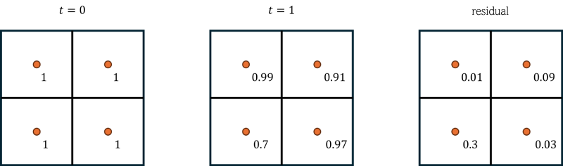
Here, I am showing what the solution values for a given quantity (this could be velocity, pressure, or temperature, for example) are at two different time steps $t=0$ and $t=1$ on the left and middle of the figure. The values are stored at the centroid, which is common for a finite volume discretisation.

On the right of the figure, I am calculating the residual based on the iteration, i.e. by how much the simulation is changing from one time step (or iteration) to the next. Say the values that I am showing in the figure are denoted by the generic quantity $\phi$ , and that the solution is given at time step $n$ (left) and $n+1$ (middle). In this case, we can compute the residual as:

\mathrm{residual}=\phi^{n+1}-\phi^{n}

Thus, for each timestep (or iteration), we can compute a residual value at each grid point for each quantity $\phi$ . This is not helping us much, as we can now say by how much the simulation is changing per quantity and per grid point, but we want to be able to judge by how much our quantity $\phi$ is changing from one timestep (or iteration) to the next.

To do so, we write all the residuals in a vector, like so:

\phi_{\mathrm{residual}}=[0.01,\,0.09,\,0.3,\,0.03]^T

In order to get a single value that represents the change from one timestep (or iteration) to the next, we can compute different vector norms. There are three common norms we use:

$L_\infty$ -norm
$L_1$ -norm
$L_2$ -norm

A vector norm is defined as follows:

|\phi|_p=\left(\sum_i |\phi_i|^p\right)^{\frac{1}{p}}

Here, $p=1, 2, ..., n$ represents the order of the norm. We saw above that the most commonly used types are the $p=1$ and $p=2$ norms. We can be written out using the above equation:

$L_1$ -norm

|\phi|_1=\sum_i |\phi_i|

$L_2$ -norm

|\phi|_2=\left(\sum_i |\phi_i|^2\right)^{\frac{1}{2}}=\sqrt{\sum_i |\phi_i|^2}

I also mentioned the special case of the $L_\infty$ -norm, sometimes also written as the $L_0$ -norm (although this may be confusing since the above definition of the vector norm does not allow a solution for $p=0$ !). This norm is defined as

|\phi|_\infty=\max_i |\phi_i|

This is a very conservative norm, as it will pick the highest residual. It does not work well with cases where we are using limiters on our numerical schemes (which we typically do). Limiters can change values in a few cells near discontinuities, for example, resulting in rather large and almost random-looking residuals. In this case, the $L_2$ -norm is better suited. For smooth solutions without the use of limiters, the $L_\infty$ -norm may be used as well.

Let’s calculate the different norms based on the residual vector we had. As a reminder, we had $\phi_{\mathrm{residual}}=[0.01,\,0.09,\,0.3,\,0.03]^T$ . Applying the various vector norms results in:

$L_\infty$ -norm

|\phi|_\infty=\max_i|\phi_{\mathrm{residual,i}}|=0.3

$L_1$ -norm

|\phi|_1=\sum_i|\phi_{\mathrm{residual,i}}|=0.01+0.09+0.3+0.03=0.43

$L_2$ -norm

|\phi|_1=\sqrt{\sum_i|\phi_{\mathrm{residual,i}}|^2}=0.01^2+0.09^2+0.3^2+0.03^2=0.0001+0.0081+0.09+0.0009=0.0991

If in doubt, use the $L_2$ -norm. It is the most robust out of the three. What we have gained now is the ability to state by how much the simulation has changed, in an average sense (at least for the $L_1$ – and $L_2$ -norm). We can now compute this residual for each quantity we are interested in (e.g. velocity, pressure, temperature) and have a mechanism to state by how much the simulation has changed for the current timestep (or iteration).

Since vector norms grow as we increase the number of grid points, we commonly apply normalisation to the residuals, which can be categorised into two different categories:

Normalise by the first residual
Normalise by the number of grid points

In the first case, we divide each residual by the residual that we computed for the first timestep (or iteration). This can be written as:

|\phi|_{\mathrm{normalised}}^n=\frac{|\phi|^n}{|\phi|^{n=0}}

Thus, by definition, we have $|\phi|^{n=0}=1$ . This is a common normalisation you will find in CFD solvers, and you can spot that easily if your residual is 1 for the first timestep (or iteration).

The second normalisation is to divide the residual by the number of grid points. This can be written as:

|\phi|_{\mathrm{normalised}}^n=\frac{|\phi|^n}{N_{\mathrm{grid}}}

Here, $N_{\mathrm{grid}}$ represents the number of cells or vertices in the solution (depending on where the solution is stored). If we store the solution at the cell centroids, as shown above, then $N_{\mathrm{grid}}$ is the number of cells. If we store the solution at the vertices instead, then $N_{\mathrm{grid}}$ is the number of vertices.

Again, we can spot this normalisation as well by inspecting our first residual. If it is not equal to one, then it has most likely been normalised by the number of cells or vertices.

This type of residual calculation is very robust. If you ever need to implement residual calculations into your own solver, then I would recommend this type. But let’s have a look at another one that you will find in CFD solvers.

Linear system of equation-based residuals

If we have to solve a linear system of equations of the form

\mathbf{A}\phi=\mathbf{b}

Then, we can use this system to calculate another type of residual. The issue with the above equation is that we have a matrix $A$ that we cannot invert easily. However, in order to solve the above system, this is exactly what we need to do. That is, if we want to solve for $\phi$ , we need to compute

\phi=\mathbf{A}^{-1}\mathbf{b}

In order to avoid the inversion of the matrix, we typically approximate this inverted matrix using some iterative procedure. In my series on how to write a CFD library in C++, we looked at the case of solving such a system. In our article, we used the conjugate gradient method to approximate $\mathbf{A}^{-1}$ .

Since we are now able to compute a solution for $\phi$ , we can also compute the following:

\phi_{\mathrm{residual}}=\mathbf{A}\phi-\mathbf{b}

The matrix $\mathbf{A}$ and right-hand side vector $b$ are known from the simulation, with $\phi$ computed, we can define a residual based on the solution of our linear system. The residual will now scale with how well we have approximated the inverse of the coefficient matrix $\mathbf{A}$ .

Since our solution vector $\phi$ is, well, a vector, we can apply the same vector norms we have introduced above to calculate a representative residual for $\phi_{\mathrm{residual}}$ .

This type of residual calculation only works if you are solving a linear system of equations, which is only the case for implicit time integrations. If you have an explicit time integration, no such system is solved, and thus, you can’t use this type of residual calculation.

Right-hand-side-based residuals

The final type of residual we will look at is very closely related to the iteration-based residual we looked at first in this section. Let us first introduce what right-hand-side-based residual means.

Whenever we have an equation and seek a numerical solution to it, we have to discretise it. We typically transform an ordinary or partial differential equation into an algebraic equation which we can solve, with the understanding that the process of approximating derivatives with numerical schemes introduces some form of modelling errors.

For example, if we take the incompressible Navier-Stokes equations, we have for the momentum equation the following form:

\frac{\partial \mathbf{u}}{\partial t}+(\mathbf{u}\cdot\nabla)\mathbf{u}=-\frac{1}{\rho}\nabla p = \nu \nabla^2\mathbf{u}

Let’s only approximate the time-derivative for the moment, using a first-order time integration for simplicity, then we have:

\frac{\mathbf{u}^{n+1}-\mathbf{u}^n}{\Delta t}+(\mathbf{u}\cdot\nabla)\mathbf{u}=-\frac{1}{\rho}\nabla p + \nu \nabla^2\mathbf{u}

We solve this equation now for the unknown velocity $\mathbf{u}^{n+1}$ , and obtain:

\mathbf{u}^{n+1}=\mathbf{u}^n + \Delta t\left[-(\mathbf{u}\cdot\nabla)\mathbf{u}-\frac{1}{\rho}\nabla p + \nu \nabla^2\mathbf{u}\right]

We can now introduce a right-hand-side vector as:

\mathbf{u}^{n+1}=\mathrm{RHS}=\mathbf{u}^n + \Delta t\left[-(\mathbf{u}\cdot\nabla)\mathbf{u}-\frac{1}{\rho}\nabla p + \nu \nabla^2\mathbf{u}\right]

This right-hand-side vector $\mathrm{RHS}$ is, well, again, a vector, and so we can apply the same vector norms introduced above.

If we bring $\mathbf{u}^n$ on the left-hand side, we obtain the following form:

\mathbf{u}^{n+1}-\mathbf{u}^n=\mathrm{RHS}=\Delta t\left[-(\mathbf{u}\cdot\nabla)\mathbf{u}-\frac{1}{\rho}\nabla p + \nu \nabla^2\mathbf{u}\right]

This resembles the first type of residual calculation we looked at above. Thus, this type is actually one and the same approach, but I thought of mentioning it here for completeness, as I have seen this used as well in the wild.

Integral quantity-based convergence

An integral quantity is a single scalar value that was computed through some form of integration. Be it a line, surface, or volume integral, all of these produce single scalar values. The lift and drag coefficients, for example, are integrated over all points on a wall boundary to yield a single quantity. Hence, the name integral quantity.

Integral quantities are representative of your solution. Just like an elected president or prime minister represents the voice of the majority of the population, an integral quantity represents the solution for a specific boundary patch (or collection thereof).

The idea of using integral quantities to judge convergences is similar to the residual-based way to judge convergence. First, we compute the integral quantities for each boundary patch and iteration. Then, we check if these quantities change less than a predefined threshold. If the change is less than the maximum allowed, we deem the solution to have converged.

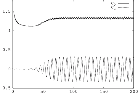
Let’s examine an example to discuss this in greater detail. The following two plots show the development of the lift coefficient overt iterations as the simulation reaches convergence.

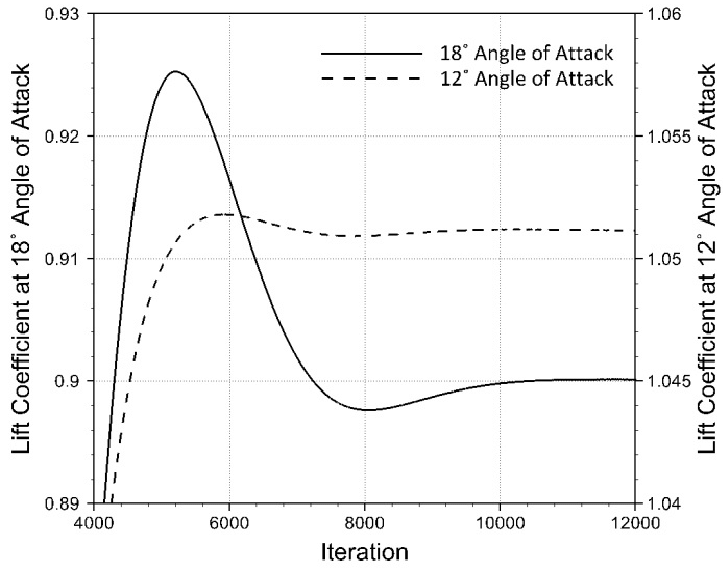
On the left plot, we see two curves for different angles of attack. We can see that around 10,000 iterations, the lift coefficient reaches an asymptotic value and likely no longer changes greatly. Thus, we may reasonably expect that the solution has converged at this point.

On the right plot, however, things are very different. We see that for the first 30-40 iterations, the simulation seems to have converged to a zero lift coefficient value. However, the lift coefficient then starts to pick up an oscillatory motion with the same frequency and amplitude. We can say that this simulation has converged to a periodic signal.

If we looked at the plot on the left and were to calculate the normalised difference in lift coefficient from one iteration to the next, we likely see that the difference after 10,000 would be rather small. We can now say that if the simulation changes by less than, say, 0.1%, we have found convergence.

But this would not work for the simulation on the right. In this case, we would never reach convergence as the integral quantity is constantly changing.

This brings us to the necessity of averaging. Integral quantities are often averaged over a few iterations, and it is this averaged quantity that is compared now. The number of iterations used to average our integral quantities is called the window size, and the averaged quantity is said to be window averaged. This is shown in the following plot.

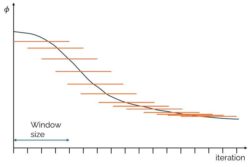
Here, we have the history of some quantity $\phi$ , which is slowly converging as the iterations increase. We now take 5 values of $\phi$ and compute its average as $\bar{\phi}^n=(\phi^{n}+\phi^{n-1}+\phi^{n-2}+\phi^{n-3}+\phi^{n-4})/5$ . This window size of 5 iterations is also shown on the bottom left of the figure.

The window averaged quantity of $\phi$ is shown by the orange lines for each iteration. We can see that as we approach the end of this fictitious simulation, the orange bars come closer together. In other words, the window averaged values are converging.

If we now calculate residual based on the window averaged quantities, we have a much more robust way to judge convergence. The residual may now be computed as:

\phi_{\mathrm{residual}}=\frac{\bar{\phi}^{n} -\bar{\phi}^{n-1}}{\bar{\phi^{n=0}}}

Here, $\bar{\phi^{n=0}}$ represents the residual at the first iteration and is used to normalise the residuals. If the condition $\phi_{\mathrm{residual}}<\varepsilon_{\mathrm{convergence-threshold}}$ is satisified, convergence is reached. Here, $\varepsilon_{\mathrm{convergence-threshold}}$ is a user-defined input.

If we return to our lift coefficient, which we saw above in the right picture, we can now introduce a window averaging procedure. If the window size contains a few of these oscillations, we can reach convergence in a window-averaged sense.

Say our window size is 50, then we capture about 8-9 periods. The average over that will likely be zero (as the mean value of the signal is centred around zero). This won’t change between window-averaged quantities, and as a result, we will reach convergence.

Judging convergence this way is much better, but it is not free from issues. Both residual- and integral quantity-based convergence checking have their respective issues that we will look at next.

Issues arising with judging convergence this way

As alluded to above, residual- and integral quantity-based convergence checking is by far the most commonly employed tactic. In this section, I want to address some of these issues, which will set us up perfectly for the framework for determining the best stopping criterion discussed in the next section.

Issue 1: Residuals and convergence do not correlate

When you are just starting with CFD, you are likely learning that when the residuals are not changing by much, your simulation has converged. You then go through some tutorials, and these do indeed converge as predicted. Later, you realise that for your own cases, you do not get convergences in this case. Why? Because tutorials typically use very simple cases for which convergence can be reached this way.

Then you start to wonder, why is my simulation no longer converging? You start to check your solver settings and cross-check them with tutorials. However, you can’t find a reason why you no longer get this nice convergence you are so used to. The truth about residuals is this:

The residuals will tell you exactly one thing, and that is if your simulation is on a path of convergence or divergence. It won’t tell you when a simulation has converged, only if it is going towards it.

If we are on a path of convergence, then our residuals are dropping in value. This is shown by residuals going down in our residual plot. If the residuals are increasing, then we are on a path towards divergence. That’s it. Using residuals to judge convergence is a common beginner mistake and one that you will avoid from now on.

There is a third case, and this is by far the most common case for high-Reynolds number flows (aka engineering applications). This is where your residuals are neither converging nor diverging but instead reaching an oscillatory motion. This motion often oscillates around the same mean value. Take the following image as an example:

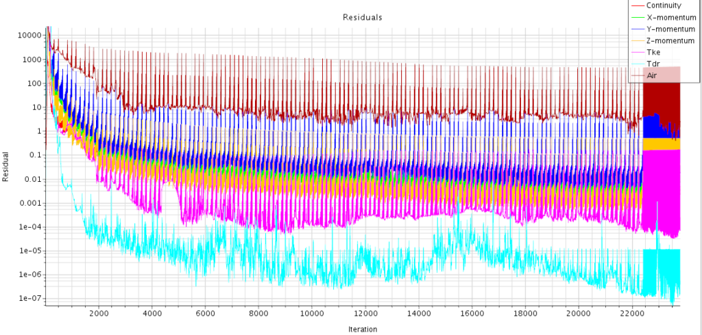
Here, all of your residuals are oscillating and using this to judge convergence is impossible. As stated above, you will most likely get this behaviour with your simulations, and thus, you want to avoid using residuals to judge convergence.

Even if the residuals are not converging, your window-averaged integral quantities will always converge, given a large enough window size. Thus, integral quantity-based convergence judging should be what you are doing from now on.

Having said that, you may be wondering, could I not use window-averaged residuals to check convergence? Yes, you can, and it would likely work, though it is not something done commonly. I can think of only one solver that will allow you to do that; in all the others, you would have to implement that type of residual checking yourself.

Thus, it is best to leave the convergence checking to integral quantities and only use residuals as an indicator for convergence, divergence, or reaching an oscillatory plateau!

Issue 2: Integral quantities only provide convergence for selected boundary patches

Say we use the lift and drag value to judge convergence on an airfoil. The integral quantities may converge at one point, and you happily stop the simulation, but you can now only say that your simulation has converged for the flow around your airfoil. Why? Because your integral quantities are based on values taken at the boundary.

Here is a test you can (and should) do next time you perform your simulations. Set up as many force coefficient monitors as feasible (i.e. lift, drag, side force, moment coefficient, etc.). Set the same window size and convergence threshold for all of them. At what time do you reach convergence? All of these quantities will converge at different points in time (iteration)!

The lift coefficient, in this case, is mainly driven by the pressure. The drag coefficient, on the other hand, is mainly driven by the velocity (gradient). Thus, if the pressure and velocity fields are converging at different rates (which they typically do), then so are our integral quantities.

So, not only does integral quantity-based convergence tell us only about convergence at the boundary patches on which they are defined, but these coefficients may also converge at different rates.

Sometimes, you need to be creative and come up with measurements that do not necessarily reveal any physical information. We use this information solely to judge convergence in a specific part of the domain (e.g., the wake).

Sticking with the airfoil example, even though our lift and drag coefficient may have converged, we have no idea if the flow in the wake has converged either. If we wanted to measure convergence in the wake, we would have to come up with another integral quantity here.

One logical integral quantity may be the integrated momentum thickness along a line embedded in the airfoil’s wake. Once the wake stabilises in an averaged sense, the window averaged integrated momentum thickness will converge. If you were to do that, and test that for a high-angle of attack flow, you would likely see very different convergence behaviour, and likely need a larger window size in the wake compared to the airfoil.

This brings us to the next issue with integral quantity-based residual checking. What is a proper convergence threshold and window size?

Issue 3: The window size and convergence threshold can lead to premature convergence

The final issue with integral quantity-based convergence judgment is that we have to specify the window size and convergence threshold. We have no idea what values to use here and have to rely entirely on our intuition, experiences, and guesstimations. If we don’t have any of that, we likely stick with the default values the solver gives us (if it has any, that is!). This is a dangerous endeavour.

Based on the window size and the convergence threshold, your simulation may reach premature convergence. I label simulations as prematurely converged if the solver suggests that results have converged, while in reality, the integral quantities would further change (and even find a new minimum or maximum) if the simulation was to be continued. Take the following plot, for example:

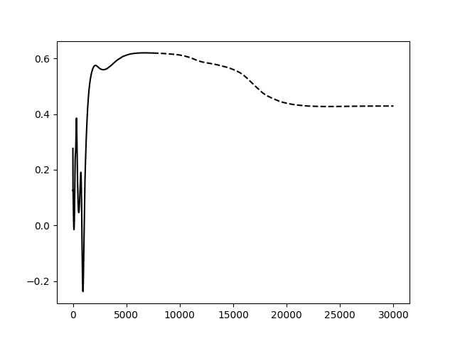
In this case, if we stopped the simulation after 7500 iterations, we may judge that the simulation has converged. This is shown with the solid black line. However, if we continue that simulation, we see that the integral quantity is changing, and instead of reaching an asymptotic limit at around 0.6, we are now reaching a new asymptotic limit at around 0.4, as shown by the black dashed line.

Thus, while integral quantity-based convergence judging is the best way to judge convergence, it does have inputs for which the wrong values can lead to premature convergence. The question then becomes, can we automate this and find the best possible window size and convergence threshold that will avoid premature convergence or at least warn us about it?

The answer is yes, and this is what we will look at in the next section.

The solution: An optimal stopping criterion framework

We have now looked at the different stopping mechanisms to judge convergence. In the following, I want to share with you my framework that can determine the window size and convergence threshold $\varepsilon_{\mathrm{convergence-threshold}}$ automatically. This allows us to avoid premature convergence while ensuring the simulation does converge.

The framework is split into five steps that need to be followed. Each step will be detailed below, but before we go through each step, let’s look at the required inputs. There are four parameters we have to specify before the framework can start calculating the best stopping criterion:

Minimum window size: This is the smallest window size that should be used for averaging. A good default value is 10.
Maximum window size: Similar to the minimum size, we also specify a maximum window size. A good default value is 100.
Window increments: This is the increment in which window sizes should be checked. A good default value is 5, and this means we would be checking window sizes of 10, 15, 20, 25, …, 85, 90, 95, and 100, if we use the default values specified above.
Asymptotic Convergence Tthreshold (ACT): This is the value used to judge if a quantity has converged to its asymptotic value. See further explanations in step 3 of this framework.

Step 1: Perform a sufficiently long, single simulation without a stopping criterion

The first step in this framework is to establish a baseline. For that, we need to run a simulation where the integral quantities do not change anymore. This is achieved by running the simulation until a clear asymptotic value has been reached. This is demonstrated in the following figure:

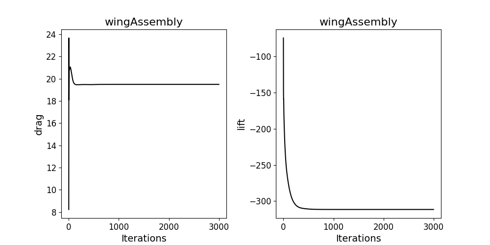
Here, it is likely that convergence is reached before 1000 iterations, though we leave the simulation running until we see a clear convergence to an asymptotic value. Here, we reach an asymptotic value of just under 20N for the drag and about -300N for lift (or downforce, in this case).

The above simulation was actually run until 20,000 iterations. I am just showing here the first 3,000 iterations, but I hope you can see that this simulation does not change anymore. The asymptotic values for 20,000 iterations do not change anymore, either.

Step 2: Calculate the asymptotic integral quantity

The next step is to calculate the asymptotic value at the end of the simulation. This is the 20N and -300N we saw above, respectively. This value will allow us to determine what the integral quantity would be if an infinite number of iterations were to be used.

In the above example, the signal appears rather clean, i.e. there aren’t any oscillations in the lift and drag values. However, as we saw before, there may always be some form of oscillation in the integral quantities. Thus, we have to average our asymptotic value over a few iterations at the end to ensure a mean value. We use the minimum window size to average the last few iterations.

Step 3: Determine the earliest iteration to stop based on the asymptotic value

Now that we have calculated what the asymptotic value of $\overline{\phi_{\mathrm{asymptotic}}}$ is, we can make comparisons against the window-averaged values $\overline{\phi_i}$ at each iteration.

One of the inputs to this framework is the Asymptotic Convergence Threshold or ACT. We use these values to check at which point our window averaged values are within a certain percentage (specified by ACT) of our asymptotic value. Once we have found this point, we label it as the earliest iteration at which the simulation can be deemed to have converged. This can be expressed as:

\frac{\overline{\phi_{\mathrm{asymptotic}}} - \overline{\phi_{\mathrm{i}}}}{\overline{\phi_{\mathrm{asymptotic}}}} < ACT

Here, $\overline{\phi_i}$ is the variable for a given iteration $i$ , which requires the above expression to be evaluated within a loop.

The following figure also shows what ACT is doing:

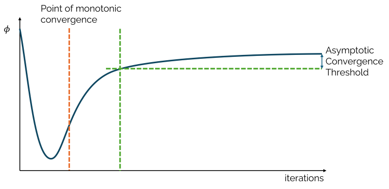
The values of $\phi$ are shown by the dark blue curve. This curve asymptotically reaches a constant value at the end of the simulation. ACT is the maximum deviation of this asymptotic value, which we allow to ensure the simulation is within this region. In the figure above, ACT is the blue double arrow line showing the maximum allowable difference from the actual asymptotic value.

We then simply check at which point the values of $\phi$ are outside of this range. We use the horizontal dashed green line to show at which point the maximum allowable difference, or ACT, intersects with our values for $\phi$ . At this point, we have found the earliest point where the simulation can be stopped.

We will use this line for the optimal stopping criterion later. If the optimal stopping criterion (which is determined by this framework) results in an iteration that is before the one determined in this step, the simulation is said to have converged prematurely. Otherwise, we have reached convergence.

Since it is common for integral quantities to change rapidly at the beginning of the simulation, with many possible over and undershoots, $\overline{\phi_i}$ may be within range of the asymptotic range value in the process. We see that $\phi$ would cross the horizontal green dashed line early on, but clearly, the simulation has not yet converged.

To avoid a false detection of asymptotic convergence, we need to avoid these regions in the beginning. We do that by looking for the point at which we are just within ACT by starting from the back (last iteration) and working our way to the front (first iteration). in this way, we know when we are leaving ACT, and so we can find the point this way.

Step 4: Determine the point of monotonic convergence

The point of monotonic convergence is a point in which the window averaged quantities are either only increasing or decreasing. It is expected that the integral quantities will fluctuate at the beginning of the simulation. However, at some point, we do expect these fluctuations to settle. It is then common for the window-averaged quantities to reach a state of monotonic convergence.

This monotonic convergence can be reached long before the earliest iteration to stop has been reached. In some cases, though, it can be also afterwards. Thus, this value should not be used to judge convergence, rather, it is an indicator for when the solution is marching towards monotonic convergence.

If the monotonic convergence is reached past the optimal iteration stop, as determined in the previous step, then this may suggest that the solution has not yet fully converged. We may need to continue our simulation to check that the asymptotic value does not change. Or, it may simply show that we have an oscillatory integral quantity, either way, we use it as an indicator only, not as a criterion to judge convergence.

In the figure above, the point of monotonic convergence is given by the orange dashed line. At this point, the solution of $\phi$ does monotonically converge towards an asymptotic value. The slope of $\phi$ is positive after this point for all values.

Step 5: Determine the optimal window size and convergence threshold that leads to convergence past the earliest iteration

This is the main work of this framework. Now that we have established the best iteration to stop, we need to check when this is achieved with a given window size and convergence threshold. Note that the best iteration to stop will be different for each integral quantity and boundary patch if we are looking at more than one boundary.

For each window size to be tested (determined by the min and max window size, as well as the window increments), calculate the window-averaged quantities and compute the difference between them between two subsequent iterations. These will form our residuals. We then have to check what the residual is at or past the earliest point of convergence, which we calculated in step 3. If this residual is lower than any other residual before the earliest point of convergence, we stop and store the window size, residual, and iteration at which convergence is reached.

We repeat this step for each window size and, once completed, check for which window size which gives us fastest convergence, i.e. the smallest number of iterations at which convergences was found.

In some cases, we may obtain smaller residuals before the point of earliest convergence, in which case, no optimal stopping criterion can be found for the current integral quantity and boundary patch. In this case, we can’t find a residual that is lower past the point of earliest convergence. If that is the case, we label this window size as producing premature convergence and check another window size.

The residual will later be used in our CFD solver to judge convergence, i.e. our residual will now be used as our convergence threshold. This process is also visualised in the figure below:

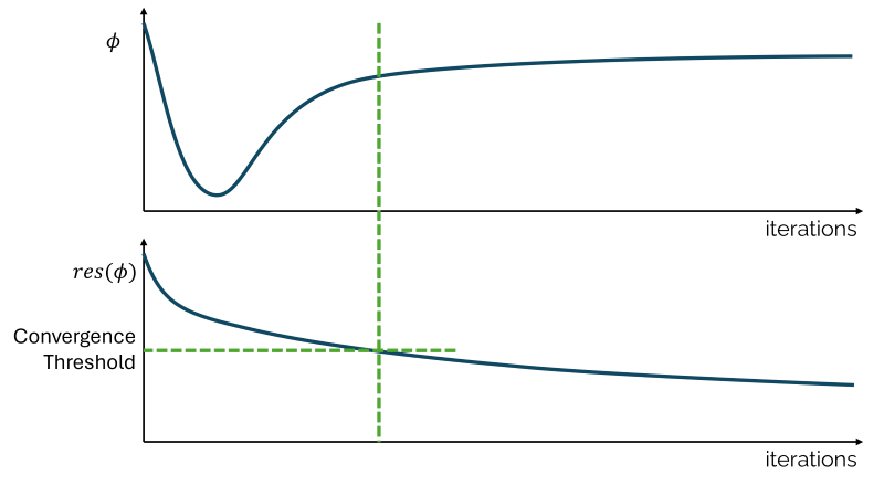
The green line represents the optimal iteration to stop (we are within a few per cent, as specified by ACT, of our asymptotic value). We then inspect the corresponding window-averaged residuals of $\phi$ , which is shown in the second plot. We look at the residual at this point and use that to set our convergence threshold (the value we have to specify in our CFD solver).

We will get different convergence threshold values for different window sizes, though we pick the one that gives us convergence closest to the optimal iteration to stop.

And this is it. We have now found a optimal iteration to stop, and determined an appropriate window size that will give us a residual (convergence threshold) close to this optimum. We can now go ahead and use these values for our integral quantity-based convergence checking.

Case studies

In this section, I want to showcase how this framework works for two separate cases. The first case is the simplest type of a Formula 1 front wing. It has an inverted and constant cambered airfoil section supplemented by an endplate. The second example is the Saab 340 turboprop aircraft at a climbing angle of attack.

Both cases will help to show how convergence is reached at different points for different integral quantities and boundaries. As a result, the framework will pick the best possible stopping criterion that works across all boundaries.

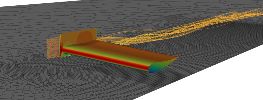
Case 1: F1-style Front Wing

The first case, as mentioned, revolves around an F1-style front wing. Well, it is simple enough to be used in class for demonstrations. You probably wouldn’t want this on your current-generation F1 cars, but I had it lying around, so let’s go with it!

I’ve given you some static pressure contour plots below of the geometry. We can also see some mesh refinement within the wing section and some streamlines that go around the endplate. These show the endplate vortex forming. Nothing spectacular, but it is a gentle introduction to see how the optimal stopping criterion framework performs.

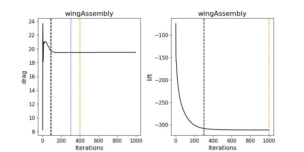
On the wing, I have recorded the lift and drag values, and the plots for them are given below. We see four different coloured lines (although a few are overlapping, so they may be difficult to differentiate). These are:

Dashed green line: This is the point at which the window-averaged integral quantity (i.e. lift or drag here) is still within 1% of the asymptotic value (here at 1000 iterations)
Dashed black line: This is the point of convergence determined by the framework. Ideally, it should be close to the green dashed line (earliest stopping point). In this case, the green and black dashed lines overlap, so they may be difficult to distinguish.
Dashed yellow line: This is the point of monotonic convergence. Drag does show monotonic convergence after 400 iterations, while lift still shows small oscillations at the last iterations. I have tested it with more than 1000 iterations, but this behaviour does not change. Monotonic convergence is always reached around the last iterations.
Dotted blue line: This looks at all boundaries (here only the wing assembly) and integral quantities (here lift and drag) and simply checks which of the black dashed lines (optimal determined stopping criterion) comes last. The simulation would, in reality, only reach convergence at this point (i.e., after all integral quantities have converged), and this line helps to visualise this point.

This provides us with a graphic representation, but we want to know what the best convergence threshold and window size are that we should use in our simulation. For that, the framework spits out the following information:

{
    "wingAssembly": {
        "drag": {
            "window_size": 15,
            "convergence_threshold": "9.1e-04",
            "iterations": 89,
            "status": "Converged"
        },
        "lift": {
            "window_size": 10,
            "convergence_threshold": "1.3e-04",
            "iterations": 301,
            "status": "Converged"
        }
    }
}

For the wingAssembly boundary patch, we have information for both the lift and drag. It tells us that convergence for the drag is reached within 89 iterations, which is achieved with a window size of 15 iterations and a convergence threshold of 9.1e-4.

The convergence status is converged, which indicates to us that using these values will make sure that convergence is reached past the earliest stopping point (that was the green dashed line in the figure above). If no optimal stopping criterion can be determined (i.e. convergence is always reached before the earliest stopping criterion), then the status will be premature convergence.

I have also shown a screenshot from ANSYS Fluent below. This is the convergence condition window, where we can impose our stopping criterion we have obtained above.

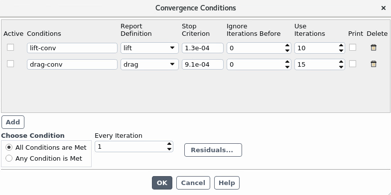
We can see that the stop criterion is the convergence_threshold the stopping criterion framework provides us. Similarly, the use iteration entry corresponds to the window_size variable in the stopping criterion framework.

We can ignore the ignore iterations before entry. Since we have already ensured that the convergence threshold and window size will give us convergence past the earliest iteration to stop, we do not need to avoid averaging over the first few iterations.

Case 2: Saab 340 aircraft during climb

The Saab 340 aircraft is another case I like to use in class, though I did generate a more refined mesh here than what I would use for demonstration. It is still relatively coarse with 25 million elements, but it will be fit for purpose for the present discussion. let’s look at some contours first to see what we can expect.

We can see the static pressure on the aircraft, and I have superimposed the Q-criterion plot (also coloured by static pressure) to see the wake development. Some mesh refinement was done around the aircraft, although some more refinement in specific areas (such as the wing tip) would have been advantageous.

The point of the Q-criterion is to visualise how the wake of the wing and the engine cover interact with the horizontal stabiliser. We can see that this wake hits the horizontal stabiliser, and as a result, we would expect the horizontal stabiliser to converge much later than the wing. This is because the wing is exposed to a clean freestream, while the horizontal stabiliser has to wait until the wing’s turbulent wake has converged.

The optimal stopping criterion framework was presented with the engine, wing, fuselage, and horizontal and vertical stabiliser boundary patches, and the lift and drag coefficients were recorded for each. The results are shown below.

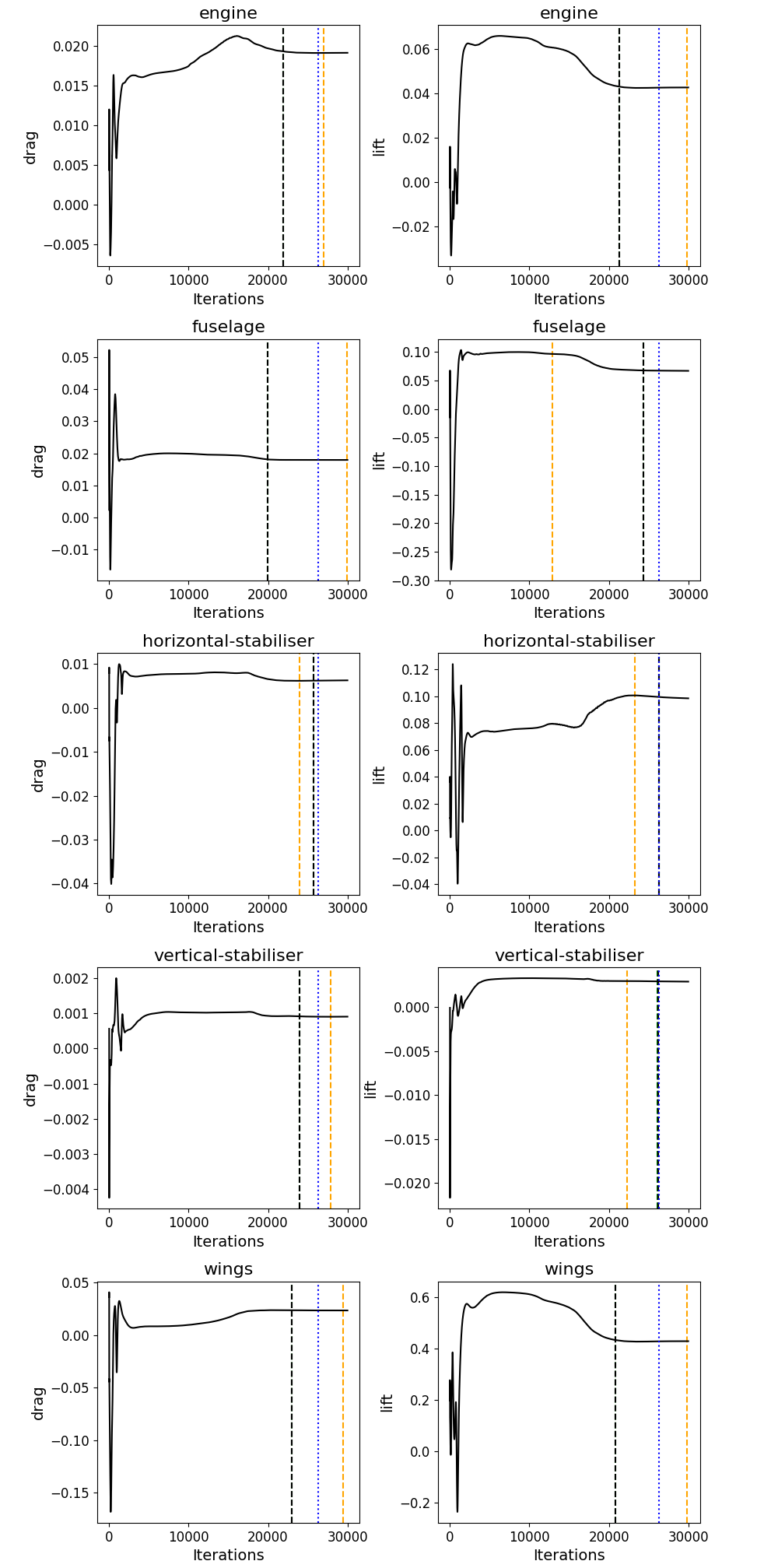
The same definitions for the coloured lines hold as for the F1-style front wing. We can see that the wing does indeed converge before the horizontal stabiliser. Convergence on the wing is reached at around 23000 iterations for the drag, while the horizontal stabiliser is only converging after 25000 iterations.

Similar outputs, as shown for the F1-style front wing, will be generated for the convergence threshold and window size (as well as a status on convergence and premature convergence). I’ll skip them here, but feel free to run this example yourself. Instructions (and all data you need) are provided on GitHub.

Summary

In this article, we reviewed the different mechanisms we have at our disposal to judge convergence. Historically, we have used residuals to judge convergence. I hope to have convinced you that residuals are only useful to see if a simulation is converging or diverging.

If we want to judge convergence, we would use integral quantities and judge when their window-averaged values no longer change. This is a much more accepted practice these days, and I recommend you start using it if you are not already doing so.

Using integral quantities, though, to judge convergence means you have to specify the window size for averaging and a convergence threshold. Both of these are difficult to determine. Intuition and experience for similar cases help here, but if you have no idea what to impose here, you ideally want to have a more generalised way to determine these inputs.

This is where the stopping criterion framework we examined comes in. Using this will allow you to determine the best possible stopping criterion for one case, which can then inform the stopping criterion for similar cases. This may work well for parametric studies.

In the end, judging convergence will ultimately be the responsibility of the CFD practitioner running the simulation. The framework developed in this article can help, but other sources, such as experimental data or reference simulation (using high-fidelity turbulence modelling), may also need to be used to judge convergence.

It is not an easy and trivial endeavour, and non-converged CFD results may sway non-CFD experts to believe that CFD is still limited in its predictive capabilities. Often, it is the user’s abuse that produces sub-optimal results. I have seen this a few times playing out in reality, and with the democratisation of CFD, we need to develop tools that will help non-CFD experts produce high-fidelity results.

This framework is my attempt to improve the convergence judgement issue, and I hope it will help you!

Tom-Robin Teschner is a senior lecturer in computational fluid dynamics and course director for the MSc in computational fluid dynamics and the MSc in aerospace computational engineering at Cranfield University.