The introduction to Large Eddy Simulations (LES) I wish I had

Regardless of whether you are a complete beginner in turbulence modelling and you are hearing the words Large Eddy Simulations (LES) for the first time today, or you are a seasoned CFD expert, I bet you that you have one thing in common: you will have gaps in your knowledge on LES.

When you read a paper or textbook on LES, the authors typically throw around integrals like candy in a carnival parade. There is so little explanation given that you stand no chance of building up an intuition for what LES really does (spoiler alert, it is rather simple). When I first studied LES, I didn’t understand much of what I was reading. It really took some time to get to the bottom of what it is actually doing. The meaning was hidden from me in plain sight behind countless unnecessarily complicated mathematical expressions.

So, while I will throw the same integrals at you in this article, I am going to slow things down. There will be lots of analogies and explanations before we even look at any equations. My goal with this article is to give you an intuition of what LES really is, not to bury you in yet more cryptic integrals. By the end of the article, you will (finally?!) understand LES from start to end.

In a sense, I have written this article to the 15-year-younger me, who would have loved to have a more explanation-driven introduction to LES. This is the introduction to LES I wish I had when I was learning about it for the first time.

This article will be a bit longer, like the others in this series as well, but I didn’t want to hold back any explanation. Make sure you have some time set aside to really take a deep dive into this subject with me. If you do, I promise you, you will see the field of turbulence modelling with a fresh view. I really hope you’ll enjoy it.

And, for what it matters, I recommend a strong brew of black tea with 2 sugars and a dash of milk. You’ll need it. Have yours ready? Good, then let’s begin our journey!

In this series

• Part 1: How to Derive the Navier-Stokes Equations: From start to end
• Part 2: What are Hyperbolic, parabolic, and elliptic equations in CFD?
• Part 3: How to discretise the Navier-Stokes equations
• Part 4: Explicit vs. Implicit time integration and the CFL condition
• Part 5: Space and time integration schemes for CFD applications
• Part 6: How to implement boundary conditions in CFD
• Part 7: How to solve incompressible and compressible flows in CFD
• Part 8: The origin of turbulence and Direct Numerical Simulations (DNS)
• Part 9: The introduction to Large Eddy Simulations (LES) I wish I had
• Part 10: All you need to know about RANS turbulence modelling in one article

In this article

Introduction

Direct Numerical Simulations are expensive. So much so that even though the first DNS appeared several decades ago, we still haven’t made much progress in the geometries we can simulate on a regular basis. We are typically still limited to simulating simplistic research geometries like a periodic box, a channel, and shear layers.

Large Eddy Simulations (LES) were introduced as a remedy. As we saw in the previous article, they cut off the turbulent energy spectrum at some wave number k, where the turbulent signal is now divided into a resolved and unresolved part. The highest wave numbers k are unresolved and require some form of modelling, while the lower wave numbers k are all resolved explicitly.

Since these lower wave numbers represent the largest (turbulent) eddies or turbulent structures in our flow, we call this turbulence modelling approach Large Eddy Simulations. Let’s see how it works in the next sections.

The main idea behind Large Eddy Simulations (LES)

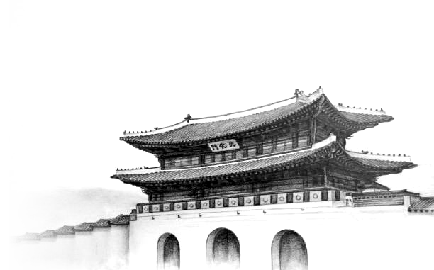
LES is all about filtering. We want to filter the flow into a resolved and unresolved part. Our computational grid acts as a filter in this case. To understand what this means, let us review some turbulent eddies in conjunction with the computational grid. This is shown in the following figure:

On the left of the figure, we see a distribution of differently sized turbulent eddies. I have colour-coded them into red and green turbulent eddies. Green eddies are large enough to be resolved by the grid, and red eddies are too small to be resolved. This is schematically shown in the figure on the right.

If we want to resolve a turbulent eddy, we need at least 4 cells (here shown in two dimensions, 8 cells in three dimensions). We need them so that the flow can turn around corners to resolve vortical motions (turbulent eddies). If the diameter of a turbulent eddy is comparable to the mesh spacing in each direction, then it will fit into a single computational cell.

Since we only use a single integration point within the finite volume method (the most common choice in CFD), we can only store one velocity component per cell, and so can’t resolve a full turbulent eddy that has a size comparable to our computational grid. If we use a finite element-based discretisation with more than one integration point per cell, i.e. higher-order cells, then we could resolve turbulent eddies again.

Thus, we can see in the figure on the right that those eddies that are of the size of the grid are effectively filtered out. You can think of the mesh as a sieve, and the turbulent eddies as a solid structure. If you put all of your turbulent eddies into the sieve, the smallest one would fall through the sieve while the largest ones would be caught by it. This is the main idea behind LES, i.e. filtering the turbulent flow into the largest, resolved turbulent eddies and the smallest, unresolved, turbulent eddies.

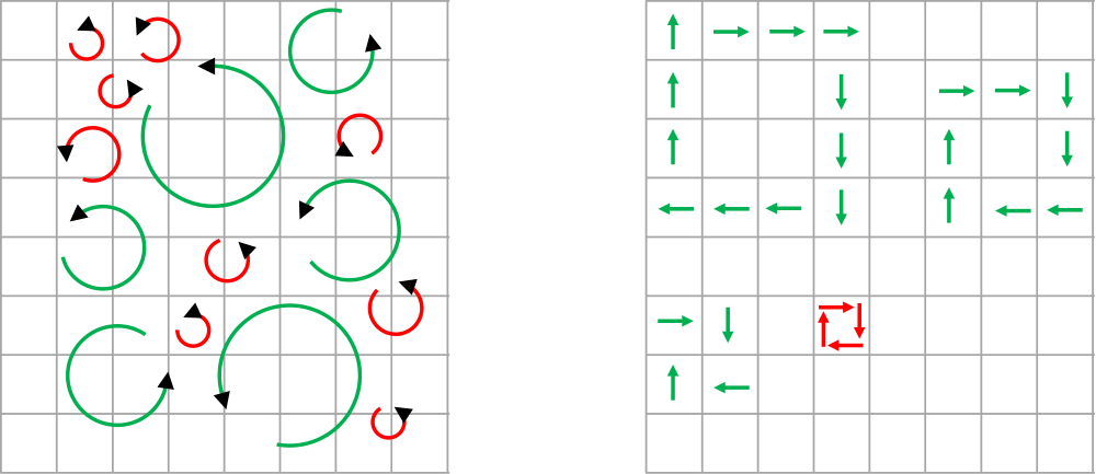
We saw this also in the turbulent energy spectrum, which I repeat below for convenience:

LES typically resolves the energy production and most of the inertial range, while the dissipation, and perhaps some of the inertial range, is modelled by LES. How is turbulence modelled here? Well, let us look at the dissipation range for that.

We said before that turbulence is generated or produced at the largest scales. This is the energy production region, and we saw that turbulence is created through the non-linear term. By taking the time-averaged form of the instantaneous momentum equation, we saw the appearance of the Reynolds stress tensor, and the energy required to feed this stress tensor is taken from the mean flow (specifically, the non-linear term).

We also said that this turbulent energy is then cascaded through a universal process, which was described by Kolmogorov, which we know as Kolmogorov’s k^{-5/3} law, which describes the slope within the inertial range. We saw that regardless of which flow we analyse, we always obtain this universal scaling of k^{-5/3}.

What happens in this inertial range from a physical point of view is that turbulent eddies are reduced in size in order to retain their (angular) velocity. Since turbulent flow consists of a number of turbulent eddies, all rubbing against each other. Friction will act against their motion and try to arrest their movement. In order to continue their movement, the eddies simply shrink in size to retain their angular velocity. This process is also known as vortex stretching.

Finally, we arrive at the dissipation range, where the turbulent eddies have become so small now, that the Reynolds number based on their angular velocity (velocity u), diameter (characteristic length L), and kinematic viscosity \nu will become one. Once we have achieved this stage, dissipation takes over, which dissipates all turbulent eddies at this length scale into heat.

So, what happens if we cut off the turbulent energy spectrum and we no longer model the smallest eddies? In this case, we never reach the dissipation range, and the smallest eddies that are resolved with our LES grid will have a Reynolds number much greater than one, based on the same parameters as discussed in the previous paragraph. This means turbulent eddies are no longer dissipated, and we will accumulate turbulent eddies at the smallest length scale (highest wave number) that our grid allows. This is not the correct physical behaviour, and so we need to destroy them.

How can we achieve that? Well, we already know that eddies will dissipate once their Reynolds number reaches one. So let’s write out the Reynolds number for the smallest turbulent eddy we can still resolve. This is given as:

\text{Re}=\frac{L_D(\omega \frac{L_D}{2})}{\nu}=\frac{L_D^2\omega}{2\nu}>1

Here, L_D is the diameter (characteristic length) of the smallest turbulent eddy we can still capture with our grid. \omega is the angular velocity, and we can compute the max velocity by multiplying it by half the diameter to get the velocity component at the outer edge of the turbulent eddy. We have already seen that this Reynolds number must be greater than one.

If we wanted to destroy these turbulent eddies, then we need to look at the Reynolds number definition and see which property we can change so that we get a Reynolds number of one again. If we achieve that, the smallest resolved turbulent eddies will dissipate again, and the correct physical behaviour is recovered.

The characteristic length (diameter L_D) is a property of the eddy, as is its angular velocity \omega, and we have no mechanism to set these as a simulation parameter. However, we can change the kinematic viscosity, which is just a material property. Thus, by adding some additional viscosity, we can achieve the desired behaviour. This new Reynolds number can be written as:

\text{Re}=\frac{L_D^2\omega}{2(\nu+\nu_{SGS})}=1

Here, we have introduced the so-called sub-grid scale (SGS) viscosity \nu_{SGS}. The role of LES is to find an approximation for the new viscosity. In essence, this viscosity accounts for the viscous contributions of all the smaller turbulent eddies that we have filtered away with our computational grid. We don’t know analytically what its value is, but we can find approximations that have been shown to recover the resolved flow field rather well. Models to compute \nu_{SGS} are called sub-grid scale (SGS) models, and various SGS models exist in the LES literature.

This is the main idea behind LES. We filter the smallest turbulent eddies away through our computational grid, which is unable to resolve them in the first place. We replace their behaviour with an SGS model, which simply computes how much additional viscosity is needed to destroy the smallest turbulent eddies that we are still able to resolve with our computational grid. The next step requires finding an expression for \nu_{SGS}, for which we first need to introduce filtering in a mathematical sense.

The need for local filtering

We have all been there; it is Friday evening, and you are craving for some snacks, ice cream, chocolate, or all of the them combined. Your local 24/7-ish shop is just down the road, but you are too lazy to walk the 10 minutes, so you take your cycle instead and arrive at the shop within 2 minutes. On the way back, it takes you 2.5 minutes, and since you enjoy CFD and have a tendency to overanalyse everything, you completely forget about the snacks that you just bought and get to work analysing why your average speed decreased.

Useless sidebar (don’t forget to delete this section before publishing the article!)

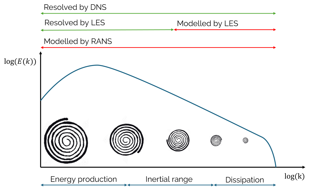
I once developed a differential equation that described how the angle between lips and the horizon (i.e. a smile) turns from positive (happy) to negative (sad) over the lifetime of the average human. The following sketch is a highly accurate mathematical description of a smile:

As we all know, a smile is defined as \Psi\ge \pi/8=22.5^\circ, i.e. if I have an eighth of a pie, I’m usually pretty happy and smile. So, that got me thinking about the general population and different cultures. Going to university in my hometown (Hamburg/Germany), I took the metro each day and over my 3 years of undergraduate studies I had a large sample pool to draw from. If you must know, the differential equation I came up with wasn’t that complex (I was an undergraduate student after all!) and given as:

\frac{\text{d}\Psi}{\text{d}t}=C_s(c)\Psi

Here, \Psi is the angle of the lips against the horizon and C_s the smile constant that depends on the culture c you draw your samples from. Here are some observations:

• The value of C_s(\text{Germany}) is always negative. Germans are born happy and die sad. I may be the first German born with a weakly positive C_s.
• The value of C_s(\text{PIGS}) is always positive (PIGS=Portugal, Italy, Greece, Spain, not an acronym I came up with!). PIGS are born happy and die at the peak of their life.
• The value of C_s(\text{USA}) is top secret.
• I could probably list more, but that would get me into hot water… let’s not go there. What is your C_s value?

So much for overanalysing every situation … Useless sidebar over, back to the main text.

It turns out, your average speed decreased because you buy snacks every Friday and exercise too little (well, you study CFD, what do you expect?). The 2 minute ride was already too much and so you slowed down on your return journey. Anyhow, it go you thinking about averages and how averaging isn’t always as simple and straight forward as it may seem.

The next day, you decide to conduct a test. Determined to get fit, you cycle 50km and measure your average speed. You managed to finish this trip in 3 hours, and your instantaneous speed at every point in time was recorded as:

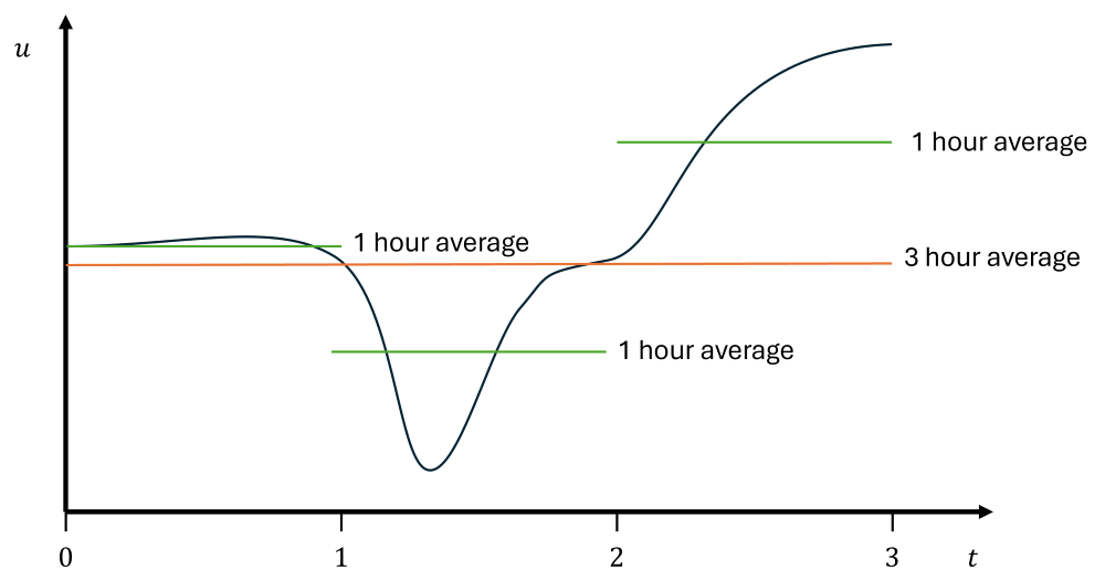
For the first hour, there was a relatively constant velocity. Flat terrain meant you could progress without issues. But then you hit a hill which you climb for the most part of the second hour, so your speed reduces. Reaching the top after 2 hours, you turn around, free-wheel down the hill and accelerated by gravity, you reach your home again within just one hour of cycling.

Obviously you could now calculate your average speed as 50 km/3h\approx 16.7\, km/h. However, if we do that, our average speed is the same everywhere, regardless of the terrain. This means our average speed is 16.7\, km/h while climbing the hill, as well as 16.7\, km/h while descending the hill. This doesn’t really make sense. So instead, you decide to compute average velocities for each leg of your trip, i.e. for the flat terrain, hill climbing, and the final descent. Your averages are now much more representative.

We could go even more granular and compute the average speed every 10 minutes, or 5 minutes, or even less. This would give us a local average speed. Why would this be important? Well, perhaps we wanted to improve our hill-climbing performance. By computing the average speed at every minute, we could have a small window over which we could check our performance and make adjustments to our power output as required.

Let’s look at another example: financial trading (something I have absolutely no idea about, but let’s give it a go). Let’s have a look at the price development of a commodity over time. This is shown in the following figure:

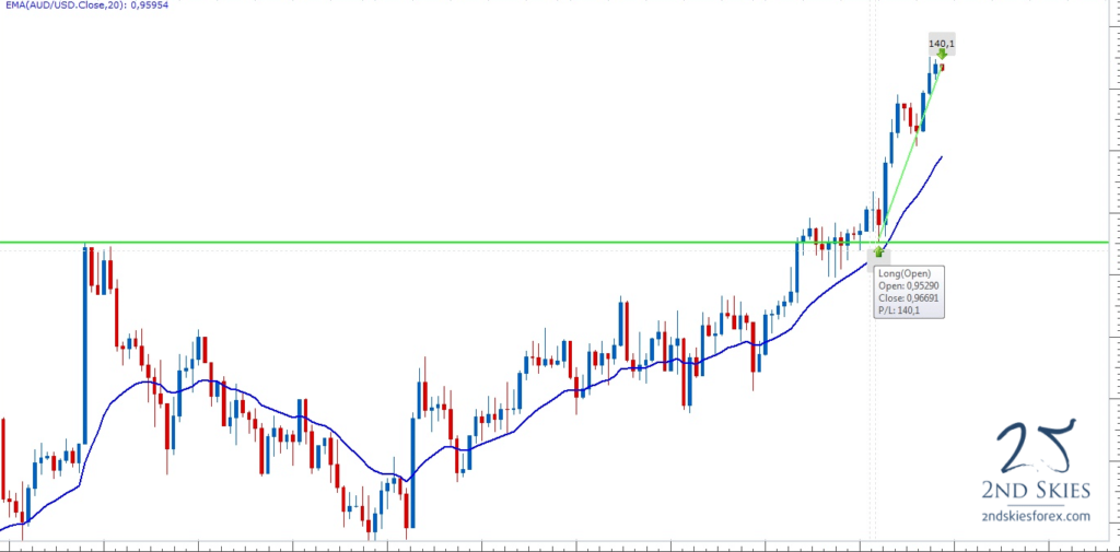
We see the price on the y-axis and how it fluctuates over time. We measure the change in price over small intervals (shown by the blue and red bars), where a blue bar means the price is increasing, and a red bar indicates that the price has dropped. The solid blue line in the background is the moving average, i.e. the local average over a small time window.

Obviously, it would make no sense to compute the average price over the last day to make a decision if you want to buy or sell stocks. Instead, you want to compute local averages, say, over the last hour, or 30 minutes, or 10 minutes, to react quickly to changes in the financial market. The solid blue line also gives you an easy way to visualise the overall trend of how the price is developing at any given point in time.

So let’s see how we could compute this average, which is also called the moving average, or running average. We could simply compute the average price \bar{p} as

\bar{p}=\frac{1}{N}\sum_{i=0}^{N-1} p_{N-i}

That is, if we have a time series of the price p, we can compute the moving average by summing up the last N values and dividing that by the number of samples N. So, for example, if we had a time history for the price of p(t)=[1, 2, 1.5, 0.8, 1, 1.2, 1, 1.8], then the average price over the last 4 samples is:

\bar{p}=\frac{1}{N}\sum_{i=0}^{N-1} p_{N-i}=\frac{1}{4}\sum_{i=0}^{3}p_{N-i}=\frac{1}{4}[1, 1.2, 1, 1.8]=\frac{5}{4}=1.25

However, if we computed the average over all samples, we would get \bar{p}=1.2875, which is slightly larger. Depending on our trading strategy, we would now know if we should buy, sell, or hold.

The moving average that we looked at assumes a discrete time series of prices in time. But what if we had an analytic function available? I.e. how can we compute the moving average for a continuous function? Well, we have to replace the discrete summation by an integral, so let’s do that:

\bar{p}=\frac{1}{T}\int_0^Tp(t)\text{d}t

Hmm, that does not look quite right. We do get the average, yes, but that is the average over the entire sample time T. We want to locally compute the average of our continuous function. No problem, we can simply multiply the instantaneous price p(t) by a function G(t) which is 1 in the sample interval during which we want to compute the average, and 0 everywhere else. Let’s define this function G as:

G(t,t',\Delta t)=
\begin{cases}
\frac{1}{\Delta t},\quad &\text{if } |t-t'|<\frac{\Delta t}{2}\\
0,\quad &\text{otherwise}
\end{cases}

Here, \Delta t is the sampling window size (e.g. 1 hour in our bicycle example), t is our time variable and t' is the time variable over which we integrate. Since we only want to integrate over some local time variable t' as we want to compute the local average, we need to differentiate between the local time variable t' and the global time variable t. These variables are shown in the following schematic view:

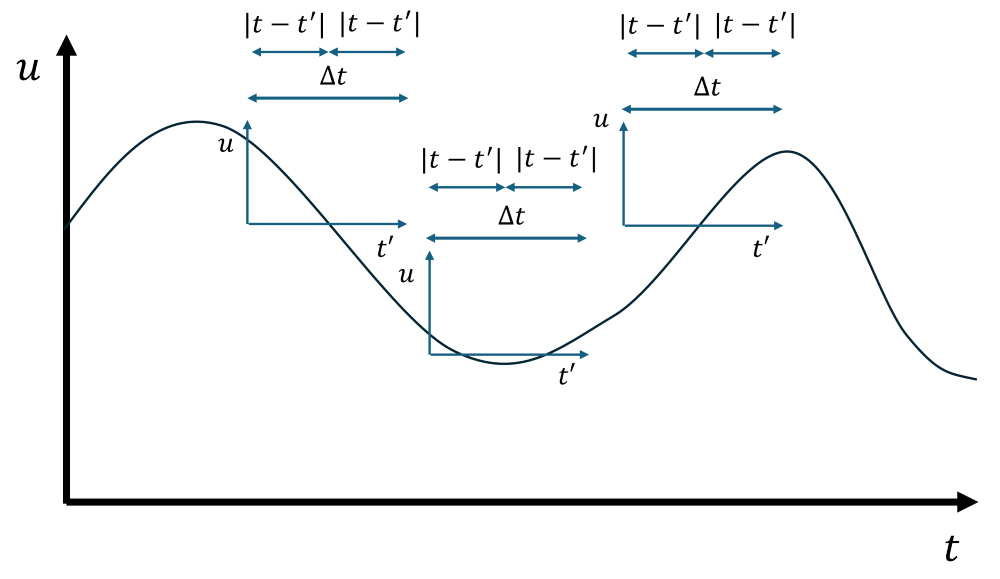
Here, for each point in time where we want to compute a local average (in this case, I have shown three), we can define a new local coordinate system that runs over t'. This coordinate runs from t'=0 to t'=\Delta t. The average of the signal u will be placed in the middle of the local coordinate system, i.e. at \Delta t / 2. We can also develop this in a graphical way, which is illustrated below:

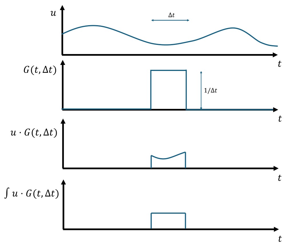
The first graph shows the global signal of u, and our goal is to compute the local average over some sampling period \Delta t. Therefore, we multiply this signal of u with the function G(t,t',\Delta t), which can be seen in the second plot. The combined signal of u\cdot G(t,t',\Delta t) is shown in the third plot. To find the average of this new combined signal, we simply integrate over this function of u\cdot G(t,t',\Delta t). This will give us a single value.

Since our integration is done in time, the units after integration will be whatever units u had (e.g. m/s) multiplied by some time variable t (i.e. seconds). To get rid of this time variable, we divide the integrated value by the sampling period \Delta t, i.e. the length in time over which we sampled. This is the same as what we did earlier in this article when we computed the time average of a signal, i.e. \bar{\phi}=(1/T)\int\phi(t)\mathrm{d}t. Here, T is the total time over which we average.

Since we have already defined the function G(t,t',\Delta t) to be 1/\Delta t in the region in which it is active, we essentially already divide by the sampling time, thus, the integral of u\cdot G(t,t',\Delta t) will be the local time average of u over the sample period \Delta t. Let us write this more formally in an integral as:

\bar{\phi}=\int_{-\infty}^\infty \phi(t)\cdot G(t,t',\Delta t)\text{d}t'

The signal \phi(t) we are considering is defined continuously in t (the entire time domain). But, we multiply it with G(t,t',\Delta t), which is only defined over some interval \Delta t in t', so this will give us the local average.

So, how does all of that relate to Large Eddy Simulations? Well, let us review a simplistic case of two individual eddies rotating. This is shown in the animation below (cue the really bad power point animations. My animation budget for today: £0. I bet you can’t tell!) :

Here, we measure the velocity v which goes in the vertical y direction at the point p over time. The two eddies we see rotate in a clockwise/counterclockwise pairing, so that at their interface, they have the same velocity component. We also advect these eddies along the horizontal x direction, going from left to right, so that they flow over the point p.

The graph below the eddies shows the recorded v velocity as the eddies pass over point p. For completeness, I have also given the velocity distribution within an eddy at the bottom right of the animation. We see that a sine wave behaviour is recovered (well, a negative cosine in this case).

What happens if we shrink these eddies down? We said angular momentum has to be conserved, so as eddies get smaller, they have to increase their angular velocity to retain the same momentum. This is shown in the next animation:

The only difference here is that the eddies spin faster, resulting in a sine wave behaviour with a higher frequency. OK, so this is all nice and fine for two eddies, but what happens if we add eddies of different sizes and angular velocity? This is (schematically) shown in the next animation:

Each eddy will now contribute its own sine wave behaviour to the global signal. Each eddy will have its own frequency based on its size, and the global velocity plot for v will appear random, while in reality, it is just a collection of sine waves (coming from all of the individual eddies).

OK, this brings us almost to LES. There is one final thing we have to cover, and that is our filtering function G(t, t',\Delta t) that we saw above. We saw that it was either switched on (having a value of 1/\Delta t) or off (having a value of 0). Because this signal, when drawn out, looks like a box, or a top-hat, this filter (sometimes also called a kernel) is known as the top-hat, or box filter/kernel. I know, mathematicians/physicists can only name things after primitive shapes or themselves! I would never do that …

We introduced this function in the context of calculating a time average, but there is nothing holding us back from applying the same computation in space, so that we get a local space average. In fact, we do it all the time, without giving it too much of a thought.

Before you leave the house, you may check the temperature outside. If you use a weather app, then the temperature you get is a local temperature average for the entire city/town/village you are living in, not the temperature in front of your door. Or, your app may say it is raining outside, while there is no rain outside your house. You might be in the 10% of the city in which it currently isn’t raining, but if there is rain in 90% of the city’s area, then it is probably fair to say that the current weather is rainy, on average.

So, similar to how we used the top-hat/box filter to define a local time average, let us also introduce the same function for a local space average in three-dimensional space. This can be expressed as:

\bar{\phi}=\int_{-\infty}^\infty \int_{-\infty}^\infty \int_{-\infty}^\infty\phi(x,y,z,t)\cdot G(x,y,z,x',y',z',\Delta x, \Delta y, \Delta z)\mathrm{d}x'\mathrm{d}y'\mathrm{d}z'

Here, this new filtering function G(x,y,z,x',y',z',\Delta x, \Delta y, \Delta z) is defined as:

G(x,y,z,x',y',z',\Delta x, \Delta y, \Delta z)=
\begin{cases}
\frac{1}{\Delta x\Delta y\Delta z},\quad &\text{if } |x-x'|\le\frac{\Delta x}{2} \,\&\, |y-y'|\le\frac{\Delta y}{2} \,\&\, |z-z'|\le\frac{\Delta z}{2}\\
0,\quad &\text{otherwise}
\end{cases}

Typically, you will see this function being introduced in a shorthand notation using G(\mathbf{x}, \mathbf{x}', \Delta\mathbf{x}) (some also write it as G(\mathbf{x}-\mathbf{x}', \Delta\mathbf{x})). Using this notation, we get:

G(\mathbf{x}, \mathbf{x}', \Delta\mathbf{x})=
\begin{cases}
\frac{1}{V},\quad &\text{if } |\mathbf{x}-\mathbf{x}'|\le\frac{\Delta \mathbf{x}}{2}\\
0,\quad &\text{otherwise}
\end{cases}

Here, V=\Delta x \Delta y \Delta z is the volume over which we average. Using this notation, we can now simplify the integral to:

\bar{\phi}=\int_{-\infty}^\infty \phi(\mathbf{x},t)\cdot G(\mathbf{x}, \mathbf{x}', \Delta\mathbf{x})\mathrm{d}\mathbf{x}

So let’s have a look at what happens when we apply this filtering to the Navier-Stokes equation, shown in a visual representation for now. The figure below shows three contour plots of the velocity, with red indicating high velocities, while blue indicates low velocities. The first image on the left is a fully resolved DNS, with all small-scale (Kolmogorov scale) fluctuations resolved.

The contour in the middle and on the right shows the same velocity fluctuations, but after we pass it through G(\mathbf{x}, \mathbf{x}', \Delta\mathbf{x}), with different sizes for \Delta \mathbf{x}. This value is smaller for the middle contour plot, resulting in a somewhat better resolution, while we have a larger value for \Delta \mathbf{x} for the contour on the right.

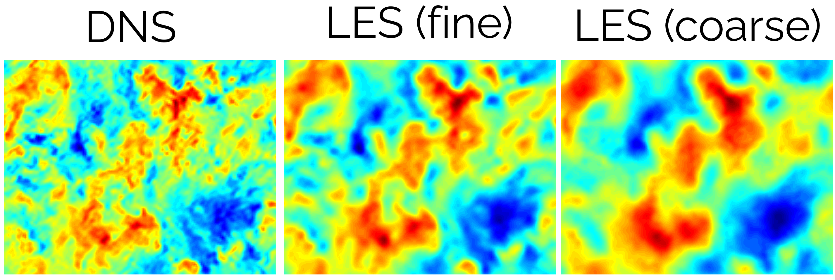
Thus, filtering is essentially the same as blurring the flow field. This gets rid of the smallest of fluctuations and only retains the largest turbulent structures (eddies). We can also see this for a 1d signal. The following plot shows a random velocity field (shown in grey) and then the filtered velocity field (i.e. the local space average) in blue:

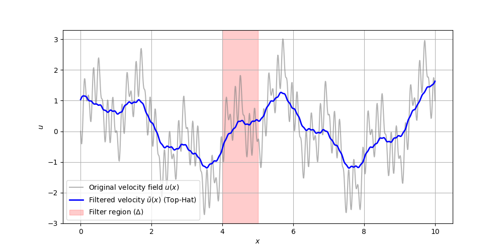
The filter width (\Delta in this case, as it is also commonly abbreviated in the LES literature, instead of using \Delta\mathbf{x}) is \Delta=1. I have shown here one filter width from 4-5, which means that the local filtered (averaged) velocity over this filtering window is obtained at x=4.5. If you look at the value we have at x=4.5, then you can see that this value is the average for all velocities within 4\le x\le 5.

We can also see now how filtering is removing the smallest scale in LES. Smaller eddies achieve one revolution much faster than larger eddies, thus their frequency is typically much higher. After we apply our filter, these higher frequencies are filtered out, meaning that we have essentially gotten rid of the small-scale fluctuations. Therefore, in LES, we see how we only contain the largest eddies, that are larger than the filtering width, which is typically computed based on the cell’s volume as \Delta=\sqrt[3]{V}=\sqrt[3]{\Delta x \Delta y \Delta z}.

For completeness, the Python code below shows how I got to this plot, so you can see how the filter is implemented as well:

import numpy as np
import matplotlib.pyplot as plt
from math import floor

# Space coordinate
x = np.linspace(0, 10, 1000)  

# Original velocity with small-scale fluctuations
u = np.sin(0.45 * np.pi * x) + np.sin(1.5 * np.pi * x) + 0.5 * np.sin(5 * np.pi * x)
u += - 0.4 * np.sin(10 * np.pi * x) - 0.5 * np.sin(15 * np.pi * x)

# Define the filter width
Delta = 1.0  # Filtering width
N = int(len(x) * Delta / (x[-1] - x[0]))  # Number of points in the filter window

# Apply the top-hat filter, reducing the filter width near boundaries
filtered_u = []
for i in range(len(x)):
    start = max(0, i - floor(N / 2.0))
    end = min(len(x), i + floor(N / 2.0))
    avg_value = sum(u[start:end]) / (end - start)
    filtered_u.append(avg_value)

# Convert list to numpy array for plotting
filtered_u = np.array(filtered_u)

# Plot the original and filtered velocity fields
plt.figure(figsize=(10, 5))
plt.plot(x, u, 'gray', alpha=0.6, label="Original velocity field $u(x)$")
plt.plot(x, filtered_u, 'b', linewidth=2, label="Filtered velocity $\\bar{u}(x)$ (Top-Hat)")
plt.axvspan(4, 4 + Delta, color='red', alpha=0.2, label="Filter region ($\\Delta$)")
plt.xlabel("$x$")
plt.ylabel("$u$")
plt.legend()
plt.grid(True)
plt.show()

The top-hat/box filter is applied on lines 17-22, where I am reducing the filter width (window) near boundaries. Thus, on the left and right side of the domain, the local filtered velocity will approach the exact value of the velocity vector, as less and less points are considered in the averaging.

Filtering is something which is barely discussed in the literature (at least in the sense where it is coming from and how our function G(\mathbf{x}, \mathbf{x}', \Delta \mathbf{x}) fits into this discussion), so I thought of being a bit more exhaustive on this topic. Hopefully, this discussion helped to develop an intuitive understanding of filtering. We will take this filter now and apply it to the Navier-Stokes equation and see what the resulting equations look like.

The filtered Navier-Stokes equations

To proceed with the filtered Navier-Stokes equation, we need to first decompose our velocity field again. This time, we filter the flow into resolved and unresolved parts. The decomposition is given as:

\mathbf{U}=\overline{\mathbf{u}}+\mathbf{u}'

Here, we have \mathbf{U} as the unfiltered, instantaneous velocity field (i.e. the full turbulence spectrum, this would be the velocity field we would obtain from a DNS). \overline{\mathbf{u}} is the resolved velocity field (the bulk flow that we are able to capture with our grid), while \mathbf{u}' is the unresolved velocity field, i.e. fluctuations arising from the smallest turbulent eddies that are smaller than our grid size.

It looks a lot like the Reynolds decomposition we looked at in the article on Direct Numerical Simulations, but it is very different. The Reynolds decomposition writes the instantaneous velocity field as a sum of a time-averaged and fluctuating velocity field, while the decomposition shown above writes the instantaneous velocity field as a spatially resolved and unresolved velocity field.

The Reynolds decomposition uses averaging in time, while the decomposition above (which we will use to derive the filtered Navier-Stokes equations for LES) uses averaging in space (over each cell volume in our grid, to be precise).

Let’s start by writing out the filtered Navier-Stokes equations. That is, we multiply each variable by our filtering function G(\mathbf{x}, \mathbf{x}', \Delta \mathbf{x}). The LES literature simply writes the filtered quantity as \overline{\phi}, which I will use here as well. We now know that this just gives us an average over the grid size, i.e. a space-averaged quantity. Then, our filtered Navier-Stokes equations, resolving only the largest eddies, can be written as:

\frac{\partial \overline{\mathbf{u}}}{\partial \mathbf{x}}=0\\[1em]

\frac{\partial \overline{\mathbf{u}}}{\partial t} + \frac{\partial \overline{\mathbf{u}} \overline{\mathbf{u}}}{\partial \mathbf{x}} = -\frac{1}{\rho}\frac{\partial\overline{p}}{\partial \mathbf{x}} + \nu\frac{\partial^2 \overline{\mathbf{u}}}{\partial \mathbf{x}^2}

Now we have one problem, and that is, that the momentum equation contains now three unknown quantities, that is, \overline{\mathbf{u}}, \overline{p}, and \overline{\mathbf{uu}}. Why is the last term, i.e. the non-linear term different from the first, i.e. \overline{\mathbf{u}}? Well, let us write out the product:

\overline{\mathbf{uu}}=\overline{(\overline{\mathbf{u}}+\mathbf{u}')(\overline{\mathbf{u}}+\mathbf{u}')}=\overline{\overline{\mathbf{u}}\,\overline{\mathbf{u}}} + \overline{\overline{\mathbf{u}}\mathbf{u}'} + \overline{\mathbf{u}'\overline{\mathbf{u}}} + \overline{\mathbf{u}'\mathbf{u}'} 

We can see here interactions of the velocity field between resolved (i.e. \overline{\mathbf{u}}) and unresolved (i.e. \mathbf{u}') part. This is shown in the following figure:

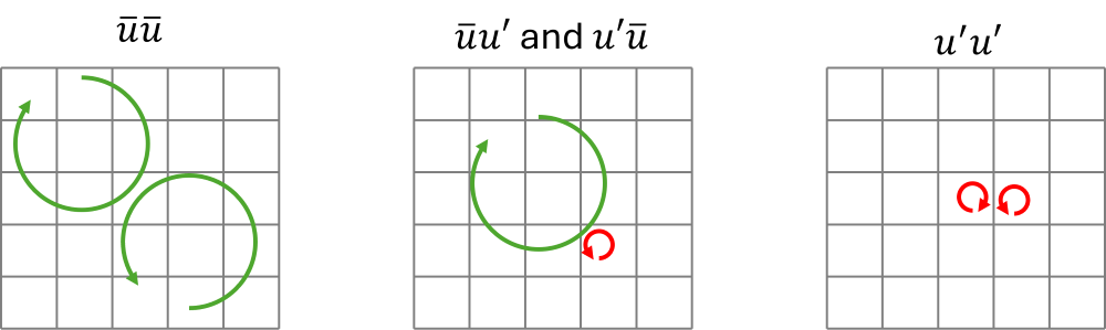
We said that the fluctuations arising from the turbulent eddies, and we said that we resolve some of them (by having a grid small enough to explicitly resolve these eddies), indicated by the contributions they make to the resolved velocity field \overline{\mathbf{u}}. Those eddies are shown in green in the figure above.

Then, we have the contributions of the smallest eddies, that we do not resolve with out grid, and these contribute the the unresolved velocity field \mathbf{u}', and those eddies are shown in red in the figure above. Thus, while we would be able to explicitly compute the resolved interactions, i.e. \overline{\overline{\mathbf{u}}\,\overline{\mathbf{u}}}, we are unable to compute the interactions between the resolved and unresolved scales, i.e. \overline{\overline{\mathbf{u}}\mathbf{u}'} and \overline{\mathbf{u}'\overline{\mathbf{u}}}, as well as the interactions on the unresolved scales alone. i.e. \overline{\mathbf{u}'\mathbf{u}'}.

Therefore, we cannot directly compute the term \overline{\mathbf{uu}} in the filtered Navier-Stokes equations. We could model this term, by deriving an additional transport equation for it, but this is not the approach taken in LES. Instead, we expand this term by adding and subtracting \bar{\mathbf{u}}\bar{\mathbf{u}}. This doesn’t change the equations, but we can use that to simplify them. Our filtered Navier-Stokes momentum equation is now:

\frac{\partial \overline{\mathbf{u}}}{\partial t} + \frac{\partial \overline{\mathbf{uu}}}{\partial \mathbf{x}} + \frac{\partial \bar{\mathbf{u}}\bar{\mathbf{u}}}{\partial \mathbf{x}} - \frac{\partial \bar{\mathbf{u}}\bar{\mathbf{u}}}{\partial \mathbf{x}}= -\frac{1}{\rho}\frac{\partial\overline{p}}{\partial \mathbf{x}} + \nu\frac{\partial^2 \overline{\mathbf{u}}}{\partial \mathbf{x}^2}

So, why did we do that? Well, we can’t explicitly compute \overline{\mathbf{uu}}, but we can compute \bar{\mathbf{u}}\bar{\mathbf{u}}. This is just multiplying the filtered (space-averaged) velocity field. This is different to applying the filter to the product of the unfiltered velocity field, i.e. we have \overline{\mathbf{uu}} \ne \bar{\mathbf{u}}\bar{\mathbf{u}}. Since we can compute that, we keep this term on the left-hand side, and we silently remove the term we can compute and place it on the right-hand side (along with the by-product \partial (\bar{\mathbf{u}}\bar{\mathbf{u}})/\partial x. This results in:

\frac{\partial \overline{\mathbf{u}}}{\partial t} + \frac{\partial \bar{\mathbf{u}}\bar{\mathbf{u}}}{\partial \mathbf{x}} = -\frac{1}{\rho}\frac{\partial\overline{p}}{\partial \mathbf{x}} + \nu\frac{\partial^2 \overline{\mathbf{u}}}{\partial \mathbf{x}^2} + \frac{\partial \bar{\mathbf{u}}\bar{\mathbf{u}}}{\partial \mathbf{x}} - \frac{\partial \overline{\mathbf{uu}}}{\partial \mathbf{x}} \\[1em]

\frac{\partial \overline{\mathbf{u}}}{\partial t} + \frac{\partial \bar{\mathbf{u}}\bar{\mathbf{u}}}{\partial \mathbf{x}} = -\frac{1}{\rho}\frac{\partial\overline{p}}{\partial \mathbf{x}} + \nu\frac{\partial^2 \overline{\mathbf{u}}}{\partial \mathbf{x}^2} + \frac{\partial \tau^{SGS}}{\partial \mathbf{x}}

Here, we have introduced a new quantity called \tau^{SGS}=\bar{\mathbf{u}}\bar{\mathbf{u}}-\overline{\mathbf{uu}}. These are the SGS (subgrid scale) stresses we can’t resolve. This contains the term \overline{\mathbf{uu}}, and we already saw how we can expand this term. Let us do that for the subgrid-scale tensor \tau^{SGS} (which for the moment is just a scalar as we are dealing with the 1D equations, but it will be a tensor in 3D) and then rearrange and label terms. We get:

\tau^{SGS}=\bar{\mathbf{u}}\bar{\mathbf{u}}-\overline{\mathbf{uu}} \\[1em]

\tau^{SGS}=\bar{\mathbf{u}}\bar{\mathbf{u}} - \overline{\bar{\mathbf{u}}\bar{\mathbf{u}}} - \overline{\bar{\mathbf{u}}\mathbf{u}'} - \overline{\mathbf{u}'\bar{\mathbf{u}}} - \overline{\mathbf{u}'\mathbf{u}'} \\[1em]

\tau^{SGS}=
\underbrace{\left(\bar{\mathbf{u}}\bar{\mathbf{u}} - \overline{\bar{\mathbf{u}}\bar{\mathbf{u}}}\right)}_\mathbf{L}
+ \underbrace{\left(-\overline{\bar{\mathbf{u}}\mathbf{u}'} - \overline{\mathbf{u}'\bar{\mathbf{u}}}\right)}_{\mathbf{C}}
+ \underbrace{\left(-\overline{\mathbf{u}'\mathbf{u}'}\right)}_{\mathbf{R}}

Here, we have grouped the terms into three separate groups:

• The Leonard stresses \mathbf{L}: These are the stresses that we can explicitly compute as these contain only quantities of the resolved velocity field.
• The cross-term stresses \mathbf{C}: These are the stresses that express the interaction of the resolved and unresolved velocity field. We cannot directly compute this.
• The Reynolds subgrid stresses \mathbf{R}: These are the interactions of the unresolved velocity field, which we are also unable to resolve explicitly.

So, now the question becomes, how do we compute the subgrid-scale tensor \tau^{SGS}? Well, we don’t! As we have already established above, we cannot compute some quantities, and in the field of CFD, whenever we cannot compute something, we either model it by analogy or remove the terms altogether and hope or pray (perhaps involving a religious sacrifice) that removing terms won’t have a strong influence.

We saw in the previous post on incompressible methods how the SIMPLE algorithm is butchering the Navier-Stokes equations in an attempt to remove everything it does not want to solve, mainly the non-linear term (when there is no need for it). We are not as creative in LES, we simply say that we can model the subgrid scale tensor by an analogy. To do that, it is going to be simpler to turn to the 3D Navier-Stokes equations (finally!). Let’s write them out here explicitly in Cartesian coordinates:

\frac{\partial \bar{u}}{\partial x} + \frac{\partial \bar{v}}{\partial y} + \frac{\partial \bar{w}}{\partial z} = 0 \\[1em]

\frac{\partial \bar{u}}{\partial t} + \frac{\partial \bar{u}\bar{u}}{\partial x} + \frac{\partial \bar{u}\bar{v}}{\partial y} + \frac{\partial \bar{u}\bar{w}}{\partial z} = -\frac{1}{\rho}\frac{\partial \bar{p}}{\partial x} + \nu\left(\frac{\partial^2\bar{u}}{\partial x^2} + \frac{\partial^2\bar{u}}{\partial y^2} + \frac{\partial^2\bar{u}}{\partial z^2}\right) + \frac{\partial \tau^{SGS}_{xx}}{\partial x} + \frac{\partial \tau^{SGS}_{xy}}{\partial y} + \frac{\partial \tau^{SGS}_{xz}}{\partial z} \\[1em]

\frac{\partial \bar{v}}{\partial t} + \frac{\partial \bar{u}\bar{v}}{\partial x} + \frac{\partial \bar{v}\bar{v}}{\partial y} + \frac{\partial \bar{v}\bar{w}}{\partial z} = -\frac{1}{\rho}\frac{\partial \bar{p}}{\partial y} + \nu\left(\frac{\partial^2\bar{v}}{\partial x^2} + \frac{\partial^2\bar{v}}{\partial y^2} + \frac{\partial^2\bar{v}}{\partial z^2}\right) + \frac{\partial \tau^{SGS}_{yx}}{\partial x} + \frac{\partial \tau^{SGS}_{yy}}{\partial y} + \frac{\partial \tau^{SGS}_{yz}}{\partial z} \\[1em]

\frac{\partial \bar{w}}{\partial t} + \frac{\partial \bar{u}\bar{w}}{\partial x} + \frac{\partial \bar{v}\bar{w}}{\partial y} + \frac{\partial \bar{w}\bar{w}}{\partial z} = -\frac{1}{\rho}\frac{\partial \bar{p}}{\partial z} + \nu\left(\frac{\partial^2\bar{w}}{\partial x^2} + \frac{\partial^2\bar{w}}{\partial y^2} + \frac{\partial^2\bar{w}}{\partial z^2}\right) + \frac{\partial \tau^{SGS}_{zx}}{\partial x} + \frac{\partial \tau^{SGS}_{zy}}{\partial y} + \frac{\partial \tau^{SGS}_{zz}}{\partial z}

Now we can see the subgrid-scale tensor in full display. Let us focus on it now. We can write \tau^{SGS} as:

\tau^{SGS}=
\begin{bmatrix}
\tau^{SGS}_{xx} & \tau^{SGS}_{xy} & \tau^{SGS}_{xz} \\[1em]
\tau^{SGS}_{yx} & \tau^{SGS}_{yy} & \tau^{SGS}_{yz} \\[1em] 
\tau^{SGS}_{zx} & \tau^{SGS}_{zy} & \tau^{SGS}_{zz}
\end{bmatrix}
=\\[1em]
\begin{bmatrix}
\bar{u}\bar{u} - \overline{\bar{u}\bar{u}} - \overline{\bar{u}u'} - \overline{u'\bar{u}} - \overline{u'u'} 
& 
\bar{u}\bar{v} - \overline{\bar{u}\bar{v}} - \overline{\bar{u}v'} - \overline{u'\bar{v}} - \overline{u'v'}
& 
\bar{u}\bar{w} - \overline{\bar{u}\bar{w}} - \overline{\bar{u}w'} - \overline{u'\bar{w}} - \overline{u'w'} 
\\[1em]
\bar{v}\bar{u} - \overline{\bar{v}\bar{u}} - \overline{\bar{v}u'} - \overline{v'\bar{u}} - \overline{v'u'} 
& 
\bar{v}\bar{v} - \overline{\bar{v}\bar{v}} - \overline{\bar{v}v'} - \overline{v'\bar{v}} - \overline{v'v'} 
& 
\bar{v}\bar{w} - \overline{\bar{v}\bar{w}} - \overline{\bar{v}w'} - \overline{v'\bar{w}} - \overline{v'w'} 
\\[1em]
\bar{w}\bar{u} - \overline{\bar{w}\bar{u}} - \overline{\bar{w}u'} - \overline{w'\bar{u}} - \overline{w'u'} 
& 
\bar{w}\bar{v} - \overline{\bar{w}\bar{v}} - \overline{\bar{w}v'} - \overline{w'\bar{v}} - \overline{w'v'} 
& 
\bar{w}\bar{w} - \overline{\bar{w}\bar{w}} - \overline{\bar{w}w'} - \overline{w'\bar{w}} - \overline{w'w'}
\end{bmatrix}

In LES, we decompose this tensor now into its isotropic and deviatoric tensor parts. The isotropic part is just the elements that are on the main diagonal, while the deviatoric part is all other components which are not on the main diagonal of the tensor. We just use fancy words here to describe the main diagonal (isotropic) and off-diagonal (deviatoric) parts of the tensor.

This decomposition can be written as:

\tau^{SGS}=\underbrace{\frac{1}{3}\tau^{SGS}\mathbf{I}}_\text{isotropic} + \underbrace{\left[\tau^{SGS}-\frac{1}{3}\text{tr}\left(\tau^{SGS}\right)\mathbf{I}\right]}_\text{deviatoric}

Here, \text{tr}\left(\tau^{SGS}\right) is the trace of tensor, that is, we are summing up the components on the diagonal. We have \text{tr}=\tau_{xx}^{SGS} + \tau_{yy}^{SGS} + \tau_{zz}^{SGS}. We’ll get back to this term shortly, but first, let’s ask why we are doing this decomposition in the first place. Well, let us look at the tensor in a 3D dimension space,

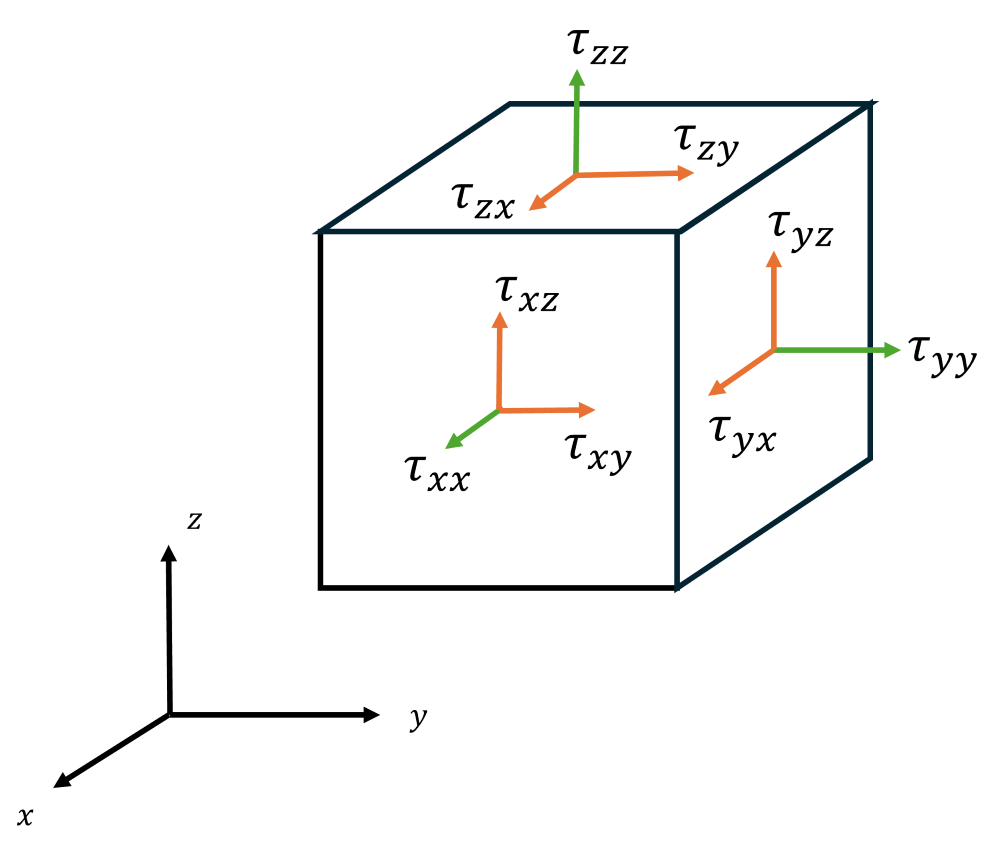
I have shown here the isotropic components in green, that is, all the subgrid-scale stresses that are on the main diagonal. The deviatoric part of the stress tensor, i.e. the off-diagonal part, is shown in orange. From this figure, we can see that the diagonal components of the tensor act normal to a plane, similar to a pressure. The off-diagonal components, on the other hand, act in-plane and are like a shearing force.

The tensor decomposition as shown above allows us to split these two separate contributions into an in-plane (deviatoric part) and normal to plane (isotropic part). Why do we have the factor of 1/3 in front of the isotropic part? The trace operator will sum up the three components on the diagonal of the tensor. We divide it by 3 (because we are in three dimensional space), to get an average of these stresses acting in each direction.

Think about the pressure. We don’t specify a pressure in the x, y, and z direction, i.e. we don’t have p_x, p_y, and p_z (although on a microscopic level, we may have p_x \ne p_y \ne p_z in certain circumstances!). Instead, we say that the pressure is a scalar value and it is acting with the same magnitude in each direction.

By taking the trace of the subgrid-scale tensor and dividing it by 3, we effectively get the same behaviour, i.e. a magnitude of the stresses. Then, we multiply it by the identity matrix \mathbf{I} so that we add this magnitude in each direction. From this decomposition, we can now bundle the isotropic part together with the pressure, where a modified pressure can be computed as:

\hat{p}=p-\frac{1}{3}\text{tr}\left(\tau^{SGS}\right)\mathbf{I}

In LES, these additional stresses are sometimes computed, but in other approaches, they are simply omitted. This leaves us with the deviatoric part of the subgrid-scale tensor. How do we model this? By analogy!

Let’s look at Newton’s law of viscosity, it states that shear stresses can be computed as a product of the viscosity and the velocity gradient. Let’s look at two examples: the flow past a flat plate and the flow past a circular cylinder. This is shown below:

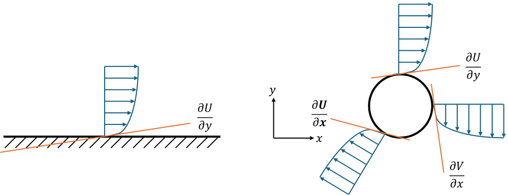
The flow is assumed to come from the left and going to the right. For the flat plate example shown on the left, we can write the definition for the shear stresses, according to Newton’s law of viscosity, as:

\tau=\mu\frac{\partial U}{\partial y}

But what about the flow past a cylinder? Once we have a curved geometry, we have a combination of derivatives. If we pick the point at the top of the cylinder, then we can find the shear stresses in the same way as we did for the flat plate. If we pick the point on the cylinder with the largest x value, then we get a different velocity gradient, as shown in the image. So, our shear stresses at this point would be computed as:

\tau=\mu\frac{\partial V}{\partial x}

But if we were to pick any arbitrary point on the cylinder, then we’ll have a combination of different gradients, which is indicated by \partial\mathbf{U}/\partial\mathbf{x}, i.e. the bold letters now stand for vector quantities, instead of scalar quantities.

To generalise the velocity gradient, so that we can take derivatives in any direction, we use the strain rate tensor in CFD. This is given as:

\mathbf{S} = \frac{1}{2} \left[ \nabla \mathbf{U} + (\nabla \mathbf{U})^{T} \right]=
\begin{bmatrix}
\frac{\partial U}{\partial x} & \frac{1}{2} \left( \frac{\partial U}{\partial y} + \frac{\partial V}{\partial x} \right) & \frac{1}{2} \left( \frac{\partial U}{\partial z} + \frac{\partial W}{\partial x} \right) \\[1em]
\frac{1}{2} \left( \frac{\partial V}{\partial x} + \frac{\partial U}{\partial y} \right) & \frac{\partial V}{\partial y} & \frac{1}{2} \left( \frac{\partial V}{\partial z} + \frac{\partial W}{\partial y} \right) \\[1em]
\frac{1}{2} \left( \frac{\partial W}{\partial x} + \frac{\partial U}{\partial z} \right) & \frac{1}{2} \left( \frac{\partial W}{\partial y} + \frac{\partial V}{\partial z} \right) & \frac{\partial W}{\partial z}
\end{bmatrix}

Thus, Newton’s law of viscosity can be generalised to \tau=2\mu \mathbf{S}, where we need to multiply by a factor of 2 now because of the 1/2 in the strain rate tensor definition.

Boussinesq postulated that the turbulent stresses, i.e. in this case \tau^{SGS} can be modelled by analogy to Newton’s law of viscosity. You may, or may not, agree with this, but this has turned out to be a useful modelling approach and turbulent stresses behave in a similar manner. Thus, we can write the turbulent stresses as:

\tau^{SGS}=
\left(\bar{\mathbf{u}}\bar{\mathbf{u}} - \overline{\bar{\mathbf{u}}\bar{\mathbf{u}}}\right)
+ \left(-\overline{\bar{\mathbf{u}}\mathbf{u}'} - \overline{\mathbf{u}'\bar{\mathbf{u}}}\right)
+ \left(-\overline{\mathbf{u}'\mathbf{u}'}\right)
=
2\mu_{SGS}\mathbf{S}

Here, we are saying that we want to model the entire subgrid scale tensor, i.e. the Leonard, cross-term, and Reynolds subgrid scale stresses completly by Boussinesq’s eddy viscosity hypothesis (as it is also known). The only modification we have done is to change the viscosity \mu to the subgrid-scale viscosity \mu_{SGS}. This accounts for the viscosity we are losing because our grid can no longer resolve the smallest eddies. Thus, we cannot simply specify this term as a material property, but instead, we need to model it.

Determining the value for \mu_{SGS} is the responsibility of the so-called subgrid-scale model, and we will review this in the next section.

Modelling approaches for the unresolved subgrid scale turbulent eddies

We are almost done! At this point, we have filtered the Navier-Stokes equation with our filtering function G(\mathbf{x}. \mathbf{x}', \Delta\mathbf{x}), so that the Navier-Stokes equations now only resolve the largest turbulent eddies. The smallest ones are filtered by the grid, as in, they are too small to resolve.

The filtering operation introduced the subgrid-scale tensor \tau^{SGS}, which we have opted to model entirely through the Boussinesq eddy viscosity hypothesis (though approaches exist that model the individual terms of \tau^{SGS} as well). We saw that Boussinesq’s hypothesis introduced the subgrid-scale viscosity \mu_{SGS}, or \mu_{SGS}/\rho=\nu_{SGS}.

Whenever we don’t know how to model an unknown, we almost always try to find other quantities that we can measure or obtain that we can use to calculate the unknown. For example, with the right equipment, we can easily measure a force. But, what if all we have is a scale to measure weight? Then, measuring a force is impossible! But, we can decompose the unknown force into F=ma=mg. We know the acceleration due to gravity g and we can measure a mass with our scale. Then we can compute the force instead of measuring it.

The same is the case for our subgrid scale viscosity \nu_{SGS}. We can’t measure it, as it accounts for the viscous dissipation that happens on length scales smaller than our grid size, so we have to decompose our subgrid scale viscosity into quantities that we can obtain or compute.

If we are tasked with finding suitable quantities that can be used to compute \nu_{SGS}, the first thing we would do is to look at its units, to figure out which other quantities we know that combine to the same units. So, for \nu_{SGS}, i.e. the kinematic subgrid scale viscosity, we have units of:

\nu_{SGS}=\left[\frac{m^2}{s}\right]

Now we need to find quantities that combined produce units of m^2/s. A naïve approach would be to simply separate the numerator and denominator. Then, we would have two quantities with units of 1/s=Hz and m^2. The first quantity has units of Hertz, i.e. a frequency, while the second has units of square meter, i.e. an area. What could be suitable choices here?

Well, in terms of the frequency, we may choose the average fluctuations of the unresolved eddies while the area could be proportional to the cell volume, i.e. V^{2/3}. While we can compute an area this way, we can’t compute the frequencies as these are for the unresolved fluctuations arising from the unresolved turbulent eddies. Since we can’t obtain this frequency (and there are probably several frequencies, i.e. several turbulent eddies of different sizes, so it isn’t clear if an average is a good idea!), this approach is not valid.

But, we can decompose the subgrid scales differently. We can also find a velocity, which has units of m/s, and a length scale, which has units of m, that combined provide us with the correct units of m^2/s. Thus, we can decompose the subgrid-scale viscosity as:

\nu_{SGS}=U\cdot l

This turns out to be a better choice, as we can find suitable approximations for the velocity and length scale. It is the job of the subgrid-scale model to find these, and we will discuss them in the next sections.

The Smagorinsky model

The Smagorinsky (sometimes also called the Smagorinsky-Lilly) model, is conceptually the simplest model to understand. As long as we stay away from solid walls, it turns out to be a pretty effective model, too! It was introduced by Smagorinsky in 1965, and saw its first use in meteorology (where near-wall effects aren’t that important).

Fun fact: Most people will cite Smagorinsky’s 1963 paper as the introduction of the Smagorinsky model but you’d struggle to find any subgrid scale model in that paper. It was the 1965 paper that gave us the Smagorinsky model (well, also not quite, we will look at this issue in the next section). But, people just cite what is written on Wikipedia, and so Smagorinsky’s 1963 paper has 10,000 citation, and his 1965 paper has about 1,500 citation as of the time of publishing this article.

To understand this model, we need to find a characteristic length scale and a characteristic velocity. To do that, let us return for a second to our sketch on the flat plate and cylinder flow:

Characteristic velocities are quite important and common in turbulence modelling, and, these are typically related to velocity gradients. As we can see for the flat plate on the left, we have only a single velocity gradient. However, the unit of a velocity gradient is [m/s]/[m]=[1/s]. In order to get units of a velocity, we have to multiply this gradient by a characteristic length scale, which we will call l for now. Then, we can define a characteristic velocity for the flat plate as U_\text{characteristic}=l\cdot (\partial U/\partial y).

When we discussed the y+ value, we were in a similar situation, where we needed to define a velocity scale. We came up with the friction velocity u_*, which was also based on the velocity gradient. In fact, this concept is so common that you will find it repeated many times throughout the history of CFD, and we will see later that the Smagorinsky model really is just a copy of another famous turbulence model. But I’m getting ahead of myself.

Let’s turn our attention to the cylinder flow now, where we see different velocity gradients. When we introduced the Boussinesq eddy viscosity hypothesis for the subgrid scale tensor \tau^{SGS}, we said that in order to capture all possible velocity gradients, we need to use the strain rate tensor, which includes all 9 possible combinations of velocities u, v, and w, as well as coordinate directions x, y, and z.

Thus, if we wanted to generalise the characteristic velocity calculation, we could replace the velocity gradient with the strain rate tensor. We would have U_\text{characteristic}=l\cdot \mathbf{S}. This is now a characteristic velocity tensor, as we multiply the scalar length scale l with the strain rate tensor \mathbf{S}, i.e. with each component of \mathbf{S}.

However, we want a single, scalar, value for the characteristic velocity. When you have a velocity vector with components in x, y, and z, and you want to determine what the velocity is in the direction it is pointing, then you would compute the magnitude of the velocity vector. The same is true for a tensor. If we wanted to know its strength (magnitude), then we compute the magnitude of the tensor. This is done in the following way:

|\mathbf{S}|=\text{mag}(\mathbf{S})=\sqrt{S_{ij}S_{ij}} = \sqrt{S_{11}S_{11} + S_{12}S_{12} + S_{13}S_{13} + S_{21}S_{21} + S_{22}S_{22} + S_{23}S_{23} + S_{31}S_{31} + S_{32}S_{32} + S_{33}S_{33}} = \\[1em]
\sqrt{S_{11}^2 + S_{12}^2 + S_{13}^2 + S_{21}^2 + S_{22}^2 + S_{23}^2 + S_{31}^2 + S_{32}^2 + S_{33}^2} = \\[1em]
\left(S_{11}^2 + S_{12}^2 + S_{13}^2 + S_{21}^2 + S_{22}^2 + S_{23}^2 + S_{31}^2 + S_{32}^2 + S_{33}^2\right)^{1/2}

We can write this out explicitly for the strain rate tensor, which yields:

|\mathbf{S}|=\text{mag}(\mathbf{S})=\sqrt{S_{ij}S_{ij}}
\\[1em]

\text{mag}\left(\begin{bmatrix}
\frac{\partial U}{\partial x} & \frac{1}{2} \left( \frac{\partial U}{\partial y} + \frac{\partial V}{\partial x} \right) & \frac{1}{2} \left( \frac{\partial U}{\partial z} + \frac{\partial W}{\partial x} \right) \\
\frac{1}{2} \left( \frac{\partial V}{\partial x} + \frac{\partial U}{\partial y} \right) & \frac{\partial V}{\partial y} & \frac{1}{2} \left( \frac{\partial V}{\partial z} + \frac{\partial W}{\partial y} \right) \\
\frac{1}{2} \left( \frac{\partial W}{\partial x} + \frac{\partial U}{\partial z} \right) & \frac{1}{2} \left( \frac{\partial W}{\partial y} + \frac{\partial V}{\partial z} \right) & \frac{\partial W}{\partial z}
\end{bmatrix}\right)=\\[1em]

\bigg[\left(\frac{\partial U}{\partial x}\right)^2 + \left(\frac{1}{2} \left( \frac{\partial U}{\partial y} + \frac{\partial V}{\partial x} \right)\right)^2 + \left(\frac{1}{2} \left( \frac{\partial U}{\partial z} + \frac{\partial W}{\partial x} \right)\right)^2 + \\[1em]
\left(\frac{1}{2} \left( \frac{\partial V}{\partial x} + \frac{\partial U}{\partial y} \right)\right)^2 + \left(\frac{\partial V}{\partial y}\right)^2 + \left(\frac{1}{2} \left( \frac{\partial V}{\partial z} + \frac{\partial W}{\partial y} \right)\right)^2 + \\[1em]
\left(\frac{1}{2} \left( \frac{\partial W}{\partial x} + \frac{\partial U}{\partial z} \right)\right)^2 + \left(\frac{1}{2} \left( \frac{\partial W}{\partial y} + \frac{\partial V}{\partial z} \right)\right)^2 + \left(\frac{\partial W}{\partial z}\right)^2\bigg]^{1/2}

If we compute now the magnitude of the strain rate tensor for the flat plate example, where the only gradient we have is \partial U/\partial y, with all other gradients being equal to zero, then we can simplify this magnitude computation to:

|\mathbf{S}|=\text{mag}(\mathbf{S})=S_{ij}S_{ij}
\\[1em]

\text{mag}\left(\begin{bmatrix}
0 & \frac{1}{2} \left( \frac{\partial U}{\partial y} \right) & 0 \\
\frac{1}{2} \left( \frac{\partial U}{\partial y} \right) & 0 & 0 \\
0 & 0 & 0
\end{bmatrix}\right)=\\[1em]

\sqrt{\left(\frac{1}{2} \frac{\partial U}{\partial y} \right)^2 + \left(\frac{1}{2} \frac{\partial U}{\partial y} \right)^2}=
\sqrt{2\cdot\left(\frac{1}{2} \frac{\partial U}{\partial y} \right)^2}=
\sqrt{2\cdot\left(\frac{1}{2}\right)^2\cdot\left(\frac{\partial U}{\partial y}\right)^2} = 
\sqrt{\frac{2}{4}\cdot\left(\frac{\partial U}{\partial y}\right)^2} = \\[1em]

\sqrt{\frac{1}{2}\cdot\left(\frac{\partial U}{\partial y}\right)^2} = 
\sqrt{\frac{1}{2}}\cdot\sqrt{\left(\frac{\partial U}{\partial y}\right)^2} = 
\frac{1}{\sqrt{2}}\frac{\partial U}{\partial y}

But, let’s have a look at the definition of the velocity gradient tensor. It is given as:

\nabla\mathbf{U}=
\begin{bmatrix}
\frac{\partial U}{\partial x} & \frac{\partial U}{\partial y} & \frac{\partial U}{\partial z} \\[1em]
\frac{\partial V}{\partial x} & \frac{\partial V}{\partial y} & \frac{\partial V}{\partial z} \\[1em]
\frac{\partial W}{\partial x} & \frac{\partial W}{\partial y} & \frac{\partial W}{\partial z}
\end{bmatrix}

Let’s compute the magnitude for this tensor, but assuming, again, that we are only considering the flat plate example, where we only have the gradient \partial U/\partial y. Then we have:

\text{mag}(\nabla\mathbf{U})=|\nabla\mathbf{U}|=\text{mag}\left(
\begin{bmatrix}
0 & \frac{\partial U}{\partial y} & 0 \\[1em]
0& 0 & 0 \\[1em]
0& 0 & 0
\end{bmatrix}\right) =
\sqrt{\left(\frac{\partial U}{\partial y}\right)^2}=
\frac{\partial U}{\partial y}

Comparing the two, we can deduce that:

\text{mag}(\nabla\mathbf{U}) \ne \text{mag}(\mathbf{S})\qquad \text{since}\qquad \frac{1}{\sqrt{2}}\frac{\partial U}{\partial y} \ne \frac{\partial U}{\partial y}

Therefore, we need multiply the magnitude of the strain rate tensor by a factor of \sqrt{2}, so that the magnitude of the velcocity gradient tensor and the strain rate is the same. Therefore, we can write our characteristic velocity scale as:

U_\text{characteristic}=\sqrt{2}\cdot \text{mag}(\mathbf{S})\cdot l=\sqrt{2}\cdot\sqrt{S_{ij}S_{ij}}\cdot l=\sqrt{2S_{ij}S_{ij}}\cdot l

Remember, a velocity gradient has units of 1/2, so we need to multiply it by some characteristic length scale l. The velocity gradient tensor is just a bunch of velocity gradients added together, so it has the same units.

If you read this and then ask yourself, well, why don’t we use the velocity gradient tensor in the first place, that’s an excelent question. To understand this, let us decompose our velocity gradient tensor in its symmetric and anti-symmetric part:

\nabla \mathbf{U} = \frac{1}{2} \nabla \mathbf{U} + \frac{1}{2} \nabla \mathbf{U}=\frac{1}{2} \nabla \mathbf{U} + \frac{1}{2} \nabla \mathbf{U}+\frac{1}{2} \nabla \mathbf{U}^T - \frac{1}{2} \nabla \mathbf{U}^T=
\\[1em]
\underbrace{\frac{1}{2} \left( \nabla \mathbf{U} + (\nabla \mathbf{U})^{T} \right)}_{\text{Symmetric (strain rate) tensor } \mathbf{S}} + 
\underbrace{\frac{1}{2} \left( \nabla \mathbf{U} - (\nabla \mathbf{U})^{T} \right)}_{\text{Antisymmetric (rotation) tensor } \mathbf{\Omega}} = \mathbf{S} + \mathbf{\Omega}

The velocity gradient tensor has been decomposed into the strain rate tensor (first term, which we have used before), and the rotational tensor \mathbf{\Omega}. The strain rate tensor is responsible for fluid deformation (through straining), while the rotational tensor is responsible for rigid body rotation.

Rigid body rotation does not add to dissipation, it is the deformation of fluid parcels that shear against one another that add to dissipation. Why is that? Well, let’s look at an analogy:

Imagine a sponge soaked with water, floating in a water bowl. If we squeeze or stretch the sponge, we change its shape and water is forced out of its pores. This will induce flow of water within the sponge and the water molecules will rub against one another, increasing shearing and thus dissipation. This is what the strain rate tensor represents (deformation of a fluid particle).

Now we are spinning the sponge. The water within the sponge will simply rotate along with the sponge, but it will stay in place. No additional internal movement of water molecules means no additional shearing force, and thus no dissipation.

Thus, since our overall goal is to find a velocity scale that multiplied by a length scale will provide us with the subgrid-scale viscosity \nu_{SGS}=l\cdot U, we need to remove the rotational tensor, as it does not add to the dissipation of the flow.

Having said that, I also mentioned that we need to correct the magnitude of the strain rate tensor by this factor \sqrt{2}. Why do we go to the extend of removing the rotational tensor if we scale the strain rate so that it is equivalent to the velocity gradient tensor?

Well, there is no precise answer here, unfortunately. Remember that the characteristic velocity scale is not an exact definition, but rather, a quantitiy that typically exists as an average of many different scales. Thus, we simply say that the strain rate is indicative of dissipation (but rotation is not, so we remove it), and in order to have a representative (characteristic) value, we ensure that it matches the velocity gradient tensor’s magnitude.

This has shown to be a good approximation. Remember that we are trying to find a model that can predict the behaviour of turbulence, we are not trying to resolve it explicitly (otherwise we would be doing a Direct Numerical Simulation (DNS)). Thus, there will always be some averaging, coming up with representative quantities, and the like, that are not exact but in the right ballpark. If this makes you still feel uneasy, then I’d strongly recommend you skip my write-up on RANS modelling. Seriously. It’s just going to get worse!

OK, let’s take stock of what we have so far. In our quest to come up with an eddy viscosity model, we said that the additional dissipation that we loose by making our grid larger so that the smallest eddies are no longer resolved can be modelled by computing a subgrid-scale viscosity \nu_{SGS}=U\cdot l. We have found an expression for the characteristic velocity U=\sqrt{2S_{ij}S_{ij}}\cdot l. Plugging that into our equation for the subgrid scale viscosity, we get:

\nu_{SGS}=l^2\cdot\sqrt{2S_{ij}S_{ij}}

So let’s talk about the characteristic length scale l. What does it physically represent? Well, let’s look at the following sketch:

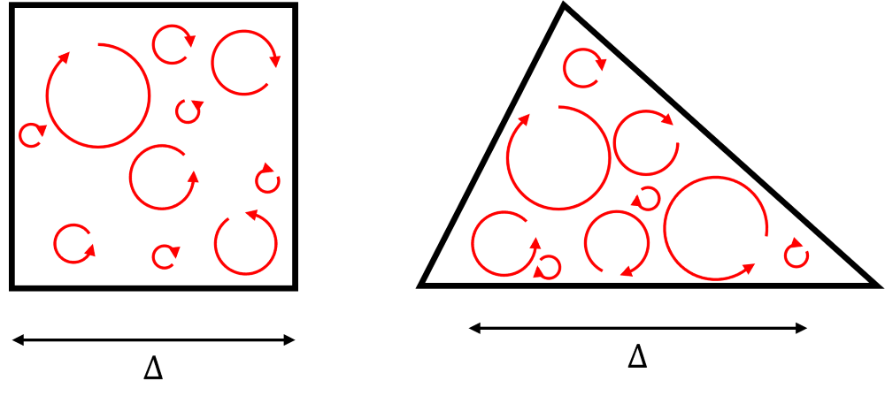
Here we see two computational cells in our mesh. One is a quad element, and the other is a triangle element, which we may encounter in an unstructured mesh. I have also shown here some unresolved eddies, that are smaller than the grid, so we can’t resolve them. We want our length scale to be representative of the average eddy size that we can’t resolve.

In three-dimensional space, each computational cell has a volume V. If we wanted to get a representative edge length of this computational cell, we could take the cube root so that we get a length with units of meters, i.e. we have L_\text{cell}=\sqrt[3]{V}.

I think L_\text{cell} is pretty descriptive, but the CFD literature disagrees. Instead, we use the symbol \Delta to indicate the average edge length of a cell in the context of LES. I find this irritating (still), as for me \Delta is just a difference operator, i.e. if we use \Delta x, we knwo this is the difference between two vertices in a mesh, which gives us the spacing in the x direction. But, since \Delta is pretty much universally adopted in the LES literature, and I want you to recognise it when you see it, we’ll use the same notation here.

If we compare the average eddy size l now against the average edge length \Delta, then we know that the following inequality must hold true: l<\Delta. Why? Because all unresolved eddies are smaller than \Delta, so their average must be smaller as well.

Inequalities aren’t nice to work with, so instead of using them, let us rewrite this in the following equation:

l=C_s\Delta

Here, we require C_s to be in the range of 0 < C_s < 1. That is, we multiply the average edge length \Delta of our computational cell with some coefficient smaller than 1 to get a representative length scale l. So, which value should we use for C_s? In all honesty, it doesn’t really matter. Every CFD solver is using their own value, and some have derived analytic expressions for it (but by assuming a very simplistic and idealised flow).

In the end, if you wanted to get an accurate value for C_s, you would need to perform a DNS first, compute the length scale l directly, make that available to an LES simulation and then compute the best value for C_s everywhere that matches your DNS data the best. But, if you already have to perform a DNS simulation, what’s the point of a lower fidelity LES simulation?

Since there is none, and the literature has a range of values suggested for C_s, typical choices for this parameter are in the range of 0.1 \le C_s \le 0.2. Because this is the Smagorinsky subgrid scale model, we also call this the Smagorinsky constant, indicated by the subscript letter s.

All that is left todo for us is to insert the definition of the characteristic length scale l, i.e. l=C_s\Delta into our definition for the subgrid scale viscosity. If we do that. we arrive at:

\nu_{SGS}=(C_s\Delta)^2\cdot\sqrt{2S_{ij}S_{ij}}

This is the Smagorinsky model in all its glory. Let’s recap how all of this fits together with the filtered Navier-Stokes equations.

First, we apply a filtering function the the Navier-Stokes equations, which we called G(\mathbf{x}, \mathbf{x}', \Delta\mathbf{x}). This resulted in the following filtered Navier-Stokes equation:

\frac{\partial \overline{\mathbf{u}}}{\partial t} + \frac{\partial \bar{\mathbf{u}}\bar{\mathbf{u}}}{\partial \mathbf{x}} = -\frac{1}{\rho}\frac{\partial\overline{p}}{\partial \mathbf{x}} + \nu\frac{\partial^2 \overline{\mathbf{u}}}{\partial \mathbf{x}^2} + \frac{\partial \tau^{SGS}}{\partial \mathbf{x}}

We saw that a new subgrid scale stress tensor appeared, which we called \tau^{SGS}. This was given as:

\tau^{SGS}=
\underbrace{\left(\bar{\mathbf{u}}\bar{\mathbf{u}} - \overline{\bar{\mathbf{u}}\bar{\mathbf{u}}}\right)}_\mathbf{L}
+ \underbrace{\left(-\overline{\bar{\mathbf{u}}\mathbf{u}'} - \overline{\mathbf{u}'\bar{\mathbf{u}}}\right)}_{\mathbf{C}}
+ \underbrace{\left(-\overline{\mathbf{u}'\mathbf{u}'}\right)}_{\mathbf{R}}

We saw that we can decompose this tensor into resolved, and unresolved parts, and while some modelling approaches exist that directly try to model the unresolved parts (i.e. the cross-term and Reynolds subgrid scale stresses), most approaches use Boussinesq’s eddy viscosity approach, in which the entire subgrid scale tensor is modelled as by an equivalent eddy viscosity \mu_{SGS}=\rho\nu_{SGS}, given as:

\tau^{SGS}=
\left(\bar{\mathbf{u}}\bar{\mathbf{u}} - \overline{\bar{\mathbf{u}}\bar{\mathbf{u}}}\right)
+ \left(-\overline{\bar{\mathbf{u}}\mathbf{u}'} - \overline{\mathbf{u}'\bar{\mathbf{u}}}\right)
+ \left(-\overline{\mathbf{u}'\mathbf{u}'}\right)
=
2\mu_{SGS}\mathbf{S}
=
2\rho\nu_{SGS}\mathbf{S}

This new subgrid scale viscosity accounts for all of the unresolved eddies that would add viscous dissipation to the flow, that we are no longer resolving. We just looked at the first (and simplest) approach to compute this subgrid scale viscosity, which we called the Smagorinsky subgrid scale model. For the sake of completeness, let’s put that here as well again:

\nu_{SGS}=(C_s\Delta)^2\cdot\sqrt{2S_{ij}S_{ij}}

If you understand this, you have mastered pretty much all there is to LES. We can now talk about different approaches to compute \nu_{SGS}, to have a better representation of the flow, but that is pretty much it.

Comparing the Smagorinsky model with Prandtl’s mixing length model

Before we continue, I want to look at Prandtl’s mixing length model, which was one of the first models used to capture the effect of turbulence. It was put forward by Prandtl in 1925, so well before we actually started doing CFD in earnest.

At the time, the Reynolds decomposition was around for a few decades, and Prandtl and his co-worker were well aware of it. The Reynolds-averaged Navier-Stokes equations were also well understood, and Prandtl tried to find a relation between the correlated Reynolds stresses \overline{u_i'u_j'} and mean flow field variables (i.e. those that could be easily measured in experiments).

Boussinesq’s eddy viscosity hypothesis was also around, and Prandtl was also well aware of it. So, Prandtl stated that the effect of the Reynold stresses could be modelled through Boussinesq’s eddy viscosity hypothesis, that is:

\overline{u_i'u_j'} = \nu_t\frac{\partial U}{\partial y}

Prandtl’s mixing length model was concerned with finding a suitable replacement for the turbulent viscosity \nu_t. He said that this could be split into two components as \nu_t=U\cdot l, where U is some characteristic velocity and l some characteristic length scale.

For the velocity, he said that a gradient multiplied by a length scale would give correct units of m/s, so he wrote:

\nu_t=U\cdot l=\bigg|\frac{\partial U}{\partial y}\bigg|\cdot l^2

Here, we are taking the absolute value of the velocity gradient so that we ensure that the turbulent viscosity remains positive. If we plug that into our eddy viscosity hypothesis, we get:

\overline{u_i'u_j'} = \nu_t\frac{\partial U}{\partial y}=l^2\bigg|\frac{\partial U}{\partial y}\bigg|\frac{\partial U}{\partial y}

This is Prandtl’s mixing length model, and, as you can see, we use the velocity gradient \partial U/\partial y here to indicate that we are dealing with a simple flow over a flat plate, for example. But there is nothing stopping us from generalising this to complex 3D flows. For this, we would first need to replace the specific gradient of U in the y direction by all possible velocity gradient combinations.

Since we already know that it is only the symmetric part of the velocity gradient tensor (i.e. the strain rate) and not the anti-symmetric part (rotation tensor) that contributes to deformation and thus dissipation, we can replace the velocity gradient in Prandtl’s mixing length model by the magnitude of the strain rate tensor. This provides us with:

\nu_t=l^2\sqrt{2S_{ij}S_{ij}}

Here, l is the so-called mixing length and, depending on the flow, takes on different values, depending on the flow we are investigating. For example, we have:

• Mixing layer: l=0.07L, with L being the layer width
• Jet: l=0.09L, with L being the half width of the jet
• Wake: l=0.16L, with L being the half width of the wake
• Outer boundary layer: l=0.09L, with L being the boundary layer height.

The list goes on, but as you can see, we have to calibrate the mixing length l for different flow scenarios. Which value should we take for l when investigating the exhaust flow of an engine? We have mixing layers, jets, wakes, and, depending on how much of the exhaust nozzle we model, boundary layers as well. For simple flows, the mixing length model is good, but it can’t handle complex flow scenarios, it is just too simplistic to represent the entire spectrum of turbulence.

So let’s compare that with the subgrid-scale model of Smagorinsky:

\nu_{SGS}=l^2\sqrt{2S_{ij}S_{ij}}

With l^2=(C_s\Delta)^2 being the length scale of the unresolved turbulent eddies. Looks familiar? How can Smagorinsky blatantly steal a different turbulence modelling approach, give it his own name, and then get away with it?

Well, in short, he never introduced a new model. Take a look at the following image, which is coming directly from Smagorinsky’s 1965 paper:

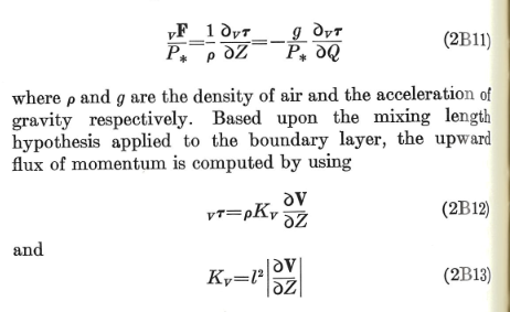
Smagorinsky explicitly states here that he is using Prandtl’s mixing length model (hypothesis). While he is using a different velocity gradient here, the Smagorinsky model is essentially just Prandtl’s mixing length model in disguise. He makes it clear and I suppose, his contribution is that he is using Prandtl’s mixing length model in a slightly different context.

Certainly, the mixing length l is different from Smagorinsky’s C_s\Delta length scale, but to me, this is a modification and not a new model in its own right. I would be OK with the name “the Prandtl-Smagorinsky model” (not because me and Prandtl are/were Germans, but because that would be a fair model name), but I suppose history is full of examples like this. Anyway, now you know, let’s move on to the next section and see how we can improve upon this simple model.

Improving upon the Smagorinsky subgrid scale model

Why do we need to improve the Smagorinsk model? Is it not already the best possible model in the universe? Not quite. Just as Prandtl’s mixing length model is too simplistic to represent the entire spectrum of turbulence, we can’t expect the Smagorinsky model to all of a sudden work wonders in the field of LES.

For starters, we have a model constant C_s for which I mentioned various values exist. The range is given as 0.1 \le C_s \le 0.2, but which value should we actually choose? Well, we could try to dynamically calculate this value, so that we get a time and space dependent value of it, i.e. C_s=f(t,\mathbf{x}). This is what Germano et al. proposed and is known as the dynamic subgrid-scale model of Germano.

Smagorinsky was primariy focused on atmospheric events, where interactions with solid walls were not important. But, in a turbulent boundary layer flow, wall effects start to become important. Here, the size of the smallest (unresolved) turbulent eddies has to decrease as we approach the wall, yet the Smagorinsky model has no mechanism for capturing this.

There are two approaches here, the first is to reduce the length scale as we approach the wall (Van Driest damping function), or, we could modify the velocity scale to account for near wall effects (WALE subgrid scale model).

Modifying the length scale: Van Driest damping function

Let us return to the law of the wall, which we looked at when we discussed the origin of turbulence and the y+ value. The law of the wall is a fundametal behaviour in turbulent flow, where we can reduce any wall-bounded flow to the same velocity profile, as long as we non-dimensionalise the velocity and wall normal distance with U^+ and y^+, respectively. A figure of this is shown in the following:

Since this is a fundamental behaviour, and it would be nice to have a uniform description of this velocity profile, different researchers have come up with their own model to describe this velocity profile, and one of the better-known ones is that of Van Driest. He showed that the velocity profile for U^+ can be expressed as:

U^+=\int_0^{y^+}\frac{2\mathrm{d}y^+}{1+\sqrt{1+4(l_m^+)^2}} \\[1em]
l_m^+=\kappa yD\\[1em]
D=\left[1-\exp\left(\frac{y^+}{A^+}\right)\right]\\[1em]
A^+=26

Here, A^+ is an empirical model coefficient and pretty much always set to A^+=26. It can be measured in experiments. l_m^+ is the mixing length (the same mixing length introduced by Prandtl), though it is modified in this context to be only valid for wall-bounded flows (e.g. turbulent boundary layers).

We see that the mixing length l_m^+ contains a parameter D, which is known these days as the Van Driest damping coefficient. If we were to plot that, with the value of D on the y-axis and the corresponding y^+ value on the x-axis, we get:

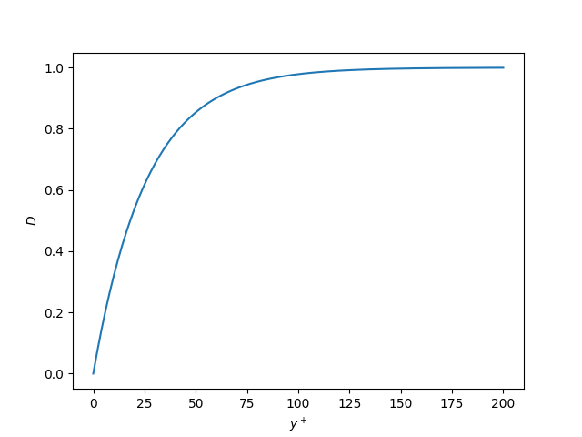
In other words, far away from the wall (y^+>100), we have D\approx 1 and so l_m^+\approx\kappa y, while for y^+<100, we have D<1 and so the mixing length l_m^+ will now get reduced. Why is this important? Let’s inspect the following figure for this:

As we approach the wall, turbulent eddies are restricted in their size. These cannot overlap with the wall, and so, we need to reduce their size as we approach the wall. This is the role of the van Driest damping coefficient D.

Let’s bring this back to the Smagorinsky subgrid-scale model. We said that the characteristic length scale l is given as l=C_s\Delta. If we are in a cell that is attached to the wall, i.e. we have y^+\approx 1 for the distance of the cell’s centroid to the wall, then l=C_s\Delta will produce eddies that are too large and overlap with the wall. This isn’t physical.

Thus, we need to scale them down, and the idea is to switch between van Driest length scale l_m^+ in cells close to the wall, and then use Smagorinsky, i.e. l=C_s\Delta away from the wall. We can achieve that by using the following expression:

l=\min(l_m^+,C_s\Delta)=\min(\kappa yD,C_s\Delta)

This leads us to the modified subgrid scale viscosity as:

\nu_{SGS}=\left[\min(\kappa yD,C_s\Delta)\right]^2\sqrt{2S_{ij}S_{ij}}

This is the van Driest damping function approach and it will ensure that eddy sizes near the wall will not be overpredicted.

Dynamic calculation of the model constant Cs: Germano’s dynamic subgrid-scale model

Since there is very little agreement in the literature over which value we should use for C_s, a natural idea may be to simply compute it and then set it for each cell, depending on which flow conditions dominate in that cell (e.g. shear flow, jet flow, wake flow, boundary layer flow, etc.)

But before we jump into the nitty gritty details of Germano’s celebrated dynamic subgrid-scale model (where C_s is now simply a function of space and time, i.e. C_s=f(t,\mathbf{x}) (congratulations, you now already know what Germano’s dynamic subgrid-scale model is)), let us start with an analogy.

When we first talked about the subgrid-scale mode \nu_{SGS}, we looked at its units and then said that we can construct a viscosity out of a length scale l and velocity scale U. That is, we replaced a quantity (the viscosity, in this case) that we can’t directly measure with two other quantities that we can.

Let’s make this even simpler. Say we want to measure the velocity of a car, but we don’t know its speed, nor can we read it off the speedometer. But, we have two images taken from a drone or helicopter that shows the car (and only that car, i.e. we have zoomed in quite a bit so that no other cars are visible). Together with a timestamp for each picture, and being able to extract the exact location by comparing the location of the car with a map (e.g. Terra Vision Google Earth), we can calculate a distance and a time difference and compute the speed as distance divided by the time taken.

This would give us exactly one piece of information, i.e. our average speed over the measured time distance, but not much more. But let’s say we take another two images at exactly the same time as the other two images, but this time we zoom out so that we can see the rest of the traffic as well.

Now we are able to not only calculate the average speed of the car we are interested in, but also the average speed of the bulk of the cars surrounding it. This allows us to extract further insights:

• The car is moving at the same average speed compared to the bulk of the cars surrounding it: The car is just following along with the traffic.
• The car is moving at a higher speed compared to the bulk of the cars surrounding it: The car picking its way through traffic, potentially breaking traffic laws (e.g. undertaking, driving faster than the speed limit, weaving, etc.)
• The car is moving at a lower speed compared to the bulk of the cars surrounding it: Congratulations, you have found me. I am probably responsible for 10% of all road rage incidents involving BMW drivers in the UK, and I am sure new BMWs are factory-fitted with silver Nissan Juke Voodoo dolls in case they encounter me.

Can we just stop for a moment and admire the absolut fever dream that is the Nissan Juke?

Well, my previous car was a Nissan Micra, I don’t have particularly good taste in cars it seems …

Where was I? Ah yes, so we have two images, one of a zoomed-in version of the car to measure its average speed accurately and one zoomed-out version to measure the average speed of the bulk of the cars surrounding it. Let’s bring that back to Smagorinsky (makes you wonder what car he was driving, doesn’t it?)

In the Smagorinsky model, we take a single-scale approach; that is, we define one velocity and one length scale. This is akin to taking one image to compute the average speed of a car. It doesn’t tell us anything about the flow we are in (shear, jet, wake, boundary layer, etc.), which in our analogy means we don’t know anything about the traffic’s behaviour (average speed of the bulk flow).

Let’s remind ourselves again how we got the this single scale approach. In the LES, we filtered the Navier-Stokes equations with a single filter and, as a result, we obtained some unresolved subgrid scales which we now model with, for example, the Smagorinsky model. The importance here is that we use a single filter and thus have to find a single length and velocity scale to model the unresolved scales. Again, this is like the single (zoomed-in) image approach to measure a car’s average speed.

If we were to introduce a second filter now into the Navier-Stokes equations, and we make the second filter much larger than the first filter, then we get some additional information about the unresolved scales. This is like zooming out and getting additional average speed information of the traffic surround the car of which we are measuring the average speed.

When we introduced the filter G(\mathbf{x}, \mathbf{x}',\Delta\mathbf{x}), we said that the filter width \Delta is of the order of the average edge length of the computational cell. In Germano’s dynamic subgrid-scale model, we introduce a second filter, the so-called test filter, where the test filter width is much larger than the original filter width, that is, \Delta^\text{test}>\Delta. This is also shown in the following figure:

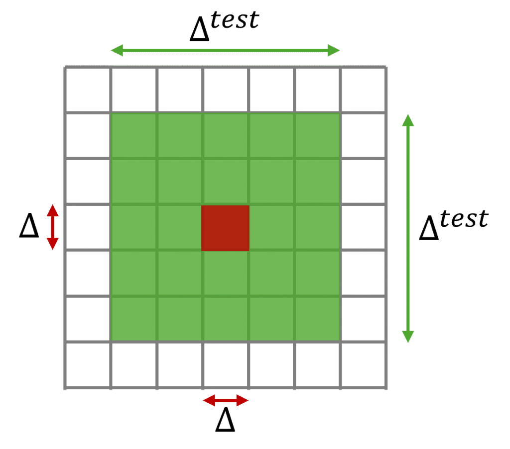
Let’s remind ourselves what the C_s coefficient embodies: It is a multiplier for the average edge length \Delta of the filtered Navier-Stokes equations, so that the product C_s\Delta returns a length scale that should match that of the unresolved turbulent eddies.

When we apply the test filter, the unresolved scales are actually resolved, as the filter width is much greater than just a single computational cell. Thus, the unresolved scales of the test filter are comparable to the resolved scales of the original filter (shown in red in the figure above). Since we now have some information on the unresolved scales, we could, in theory, compute the value C_s=l^\text{test}/\Delta, where I have simply solved for the C_s coefficient in the length scale definition we used in Smagorinsky’s original model.

We don’t actually compute the C_s coefficient this way (it is a bit more involved as we are dealing with tensors here), but the main idea is the same; construct a test filter which is larger than the original filter so that unresolved scales of the test filter are resolved by the original filter. Use that information to compute a value of C_s for each cell at each time step as we have some idea about the unresolved scales now.

Let’s look at Germano’s model in equation form now. Hopefully, with the analogy provided above, as well as some additional explanations, this will make sense now. We start with the subgrid scale tensor, that occurred after we filtered the Navier-Stokes equations. We had:

\tau^{SGS}=\bar{\mathbf{u}}\bar{\mathbf{u}}-\overline{\mathbf{u}\mathbf{u}}

These stresses appeared after we applied our filtering function G(\mathbf{x}, \mathbf{x}', \Delta\mathbf{x}) to the Navier-Stokes equation. Now we filter these equations again, with the test filter, where the test filter width is larger than the original filter, as we have established, i.e. we have \Delta^\text{test}>\Delta. A typical value is 2\Delta=\Delta^\text{test}. If we filter the already filtered Navier-Stokes equation again with our test filter, then we get:

\tau^{SGS}_\text{test}=\tilde{\bar{\mathbf{u}}}\tilde{\bar{\mathbf{u}}} - \widetilde{\overline{\mathbf{u}\mathbf{u}}}

Remember, this test filtering is like zooming out on our car to measure not just the car’s velocity, but also the bulk traffic’s average velocity in our analogy. Now we have to make use of the so-called Germano identity. We define the Leonard stresses as:

\mathbf{L} = \tilde{\bar{\mathbf{u}}}\tilde{\bar{\mathbf{u}}} - \widetilde{\bar{\mathbf{u}}\bar{\mathbf{u}}}

Where did this come from? Remember that in the original subgrid-scale model, we said that the term \mathbf{\bar{u}}\mathbf{\bar{u}} is resolved, and thus part of the Leonard stresses (which are just the resolved stresses). When we apply the test filter to the already filtered Navier-Stokes equation (which is denoted by the tilde in this case, i.e. (\tilde{\cdot})), then this term will get filtered again, which results in \tilde{\bar{\mathbf{u}}}\tilde{\bar{\mathbf{u}}}, as we can see from the first term in the test-filtered subgrid scale tensor.

Since we filter the already filtered Navier-Stokes equations, the first term in the original filtered subgrid scale tensor, i.e. \bar{\mathbf{u}}\bar{\mathbf{u}} gets filtered again, resulting in \widetilde{\bar{\mathbf{u}}\bar{\mathbf{u}}}. In the original filtered subgrid scale tensor, we said that we can’t resolve this quantity (i.e. the second term in \tau^{SGS}. But, in the test filter, we do know the filtered quantities \bar{\mathbf{u}}, as \mathbf{u} is known from the original filtering.

Therefore, we can compute the Germano identity \mathbf{L} = \tilde{\bar{\mathbf{u}}}\tilde{\bar{\mathbf{u}}} - \widetilde{\bar{\mathbf{u}}\bar{\mathbf{u}}} directly. But why would that make sense?

Let’s consider another analogy. Let’s say we are looking at a portrait of someone with a blue sky in the background. We said that LES is like blurring the flow field of a DNS simulation. If we apply the test filter, that is like blurring the already blurred flow field some more. If we apply that to our portrait, applying the first test filter is like blurring the image, and the second test filter will blur the portrait a bit more. Blurring is just taking the average of neighbouring cells (pixels), and we can increase the number of cells (pixels) to get stronger blurring.

The resolved Leonard stresses (Germano identity) tell us the difference between the two blurred flow fields. So, we could also calculate this for the two blurred images. If we looked at the sky, which has a pretty much continuous color on a pixel level, then it doesn’t really matter how much blurring we apply. The difference between the blurred images will be pretty much zero.

But, if we concentrait on small features in the portray, for example, the face, hairs, and other features, we have changes from pixel to pixel and thus the difference between different levels of blur will not be zero. This means if there are lots of small features in the image, we get a non-zero value for the difference of the blurred image, and, if we relate that back to our Leonard stresses, if we have lots of changes on the small scales in the flow field, then the difference in the Leonard stresses will not be zero.

Thus, the Germano identity tell sus something about the level of activity within the flow. If it is zero, we have undisturbed (freestream) flow, while close to walls, in jets, wakes, shear layers, etc., we have lots of motions on the small scales, which result in a non negative Leonard stress \mathbf{L}.

What we can do now is to write out the Leonard stresses explicitly, where we replace them by the eddy viscosity assumption (which was \tau^{SGS}=2\nu_{SGS}\mathbf{S}. This results in:

\mathbf{L} = \tilde{\bar{\mathbf{u}}}\tilde{\bar{\mathbf{u}}} - \widetilde{\bar{\mathbf{u}}\bar{\mathbf{u}}}=(2\nu_{SGS}\mathbf{S}^\text{original}) - (2\nu_{SGS}\mathbf{S}^\text{test}) = \\[1em] 2\underbrace{(C_s\Delta)^2\sqrt{2\mathbf{S}^\text{original}\mathbf{S}^\text{original}}}_{\nu_{SGS}}\mathbf{S}^\text{original} - 2\underbrace{(C_s\Delta^\text{test})^2\sqrt{2\mathbf{S}^\text{test}\mathbf{S}^\text{test}}}_{\nu_{SGS}}\mathbf{S}^\text{test} = \\[1em]
C_s^2\underbrace{\left(2(\Delta)^2\sqrt{2\mathbf{S}^\text{original}\mathbf{S}^\text{original}}\mathbf{S}^\text{original} - 2(\Delta^\text{test})^2\sqrt{2\mathbf{S}^\text{test}\mathbf{S}^\text{test}}\mathbf{S}^\text{test} \right)}_\mathbf{M} \\[1em]
\rightarrow \mathbf{L} = C_s^2\mathbf{M}

All the quantities in the \mathbf{M} tensor are known; therefore, we can now compute the Smagorinsky coefficient dynamically at each grid point.

But, it is not as easy as simply saying C_s^2 = \mathbf{L}/\mathbf{M}. Remember, both \mathbf{M} and \mathbf{L} are three by three tensors, therefore, we can construct nine separate equations for C_s^2. This means this problem is over-constrained.

In order to solve this problem, imagine now that we know all values of \mathbf{M} and \mathbf{L}. Then, we can plot them, where values for \mathbf{M} go on the x-axis and \mathbf{L} on the y-axis. This is visualised in the following:

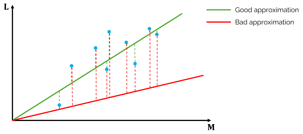
Here, all nine values of both tensors are plotted against each other, that is, we go into each tensor and then create pairs like (L_{11},M_{11}), (L_{12},M_{12}), (L_{13},M_{13}), (L_{21},M_{21}), (L_{22},M_{22}), (L_{23},M_{23}), (L_{31},M_{31}), (L_{32},M_{32}), and (L_{33},M_{33}). These are shown as blue dots.

If we wanted to describe the best fit through these points, we can try to put a line through them that minimises the distances between the blue dots and the line itself. I have shown two examples, one of a good approximation (green), and one of a bad approximation (red). I have also visualised the differences between these two lines and the dots, indicated by the dashed lines in the same colours as the lines.By just looking at the green and red distances, we can see that the green line will minimise the distance between line and dots. This will lead to a better approximation.

In a mathematical sense, if we want to achieve that, we have to use the least square approach, which will do this for us. This will compute these distances shown as dashed lines and then find whichever approximation results in the shortest distances across all points. To start, we first write the equation that we came up with above as:

(\mathbf{L}-C_s^2\mathbf{M})=0

The line that we will fit through the points in the plot will not satisfy this equation (that would mean that the line would pass through all points exactly). Thus, the right-hand side will not be zero, but instead, the distance at each dot to the line. Thus, minimising the distance will get us the closest to the above equation, as this would be closest to zero (right-hand side).

Thus far, I have kept the square in the Smagorinsky coefficient, i.e. C_s^2. However, this is dropped in many derivatives. I will introduce the substitution C=C_s^2 before continuing, so that the equation we obtain look the same to what you would find in the literature. Doing this, the minimisation process can now be expressed as:

\text{Minimise }E(C)=\sum_{i}^3\sum_j^3(L_{ij}-CM_{ij})^2

The minimum is found by setting the derivative with respect to C of this expression to zero. Why? The above equation expresses the distances between the values of L_{ij} and M_{ij} to the closest line that goes through these points. If the derivative with respect to C is zero, then there are no more changes in distances, meaning that we have found an optimum.

Another way of seeing this is to realise that L_{ij}=C_s^2M_{ij} looks a lot like the canonical form of a line expressed as y=b+mx, where in our case y=L_{ij}, b=0, m=C_s^2, and x=M_{ij}. Thus, we can think of C_s^2 (or C) as the slope of the line that fits best through all dots.

Thus, if the derivative of E(C) with respect to C does not change anymore, that means that the slope of the line does not change anymore. As a result, we have found the best fit, since the equation for C is expressed to minimise the distances between all dots and the line.

So, let’s find the derivative. We can write:

\frac{\text{d}E(C)}{\text{d}C}=\sum_i^3\sum_j^3 2(L_{ij}-CM_{ij})M_{ij}=0

This expression will minimise the distances, and thus find the optimal slope C (which will be the best coefficient to use locally in our flow field as the Smagorinsky constant). Therefore, we can compute C now from it, which is expressed as

2(L_{ij}-CM_{ij})M_{ij} \rightarrow C=\frac{L_{ij}M_{ij}}{M_{ij}M_{ij}} \\[1em] C_s^2=\frac{L_{ij}M_{ij}}{M_{ij}M_{ij}}

This is the essence of Germano’s dynamic subgrid-scale model. We have found an equation to dynamically compute C=C_s^2 by applying a coarser second filter, which we have named the test filter.

Before we close this section, you will find variations of C_s^2 in the literature. Sometimes, it is given in the same form I have derived here (see Scholarpedia, for example), other times, you may get a minus sign (depending which filtering process you subtract, i.e. either the original filter or the test filter) and even a factor of 1/2 in the definition for C_s^2 (see cfd-online, for example).

It doesn’t really matter as long as we are consistent in our derivation. The equation for C_s^2 isn’t really what we use anyway in LES. Why? Remember that the above computation is just a least square fit, i.e. there will still be some error in computing C_s^2. This can lead to strong fluctuations in the computation of C_s^2 if we look at it for a single point in space and how it evolves over time. Even worse, the value can become negative, so that instead of destroying turbulent kinetic energy, it is producing it now.

To overcome this, we need to modify this, either by clipping negative values (setting C_s^2=0 if it is computed to be negative), or by taking an average of it over a few cells in 3D space. We coudl also apply a combination of both, or we could retain the history of C_s^2 in time, to ensure that we do not have wildely fluctuating values in time (i.e. perform some kind of time averaging on top of space averaging).

Thus, if we have a factor of 1/2 in the equation for C_s^2, it doesn’t really matter, as C_s^2 will most likely get modified anyways, and the equation for C_s^2 simply represents a starting point.

Modifying the velocity scale: Wall adaptive local eddy (WALE) viscosity model

Let’s look at Smagorinsk’s subgrid-scale model again, which was inspired by Prandlt’s mixing length model:

\nu_{SGS}=l\cdot U=(\underbrace{C_s\Delta}_l)^2\cdot\underbrace{\sqrt{2S_{ij}S_{ij}}}_U

Smagorinsky said that the velocity scale can be approximated by the magnitude of the strain rate tensor. Let’s look at the definition of the strain rate tensor then again:

\mathbf{S}=S_{ij}=(\nabla\mathbf{U}+(\nabla\mathbf{U})^T)=\begin{bmatrix}
\frac{\partial U}{\partial x} & \frac{1}{2} \left( \frac{\partial U}{\partial y} + \frac{\partial V}{\partial x} \right) & \frac{1}{2} \left( \frac{\partial U}{\partial z} + \frac{\partial W}{\partial x} \right) \\
\frac{1}{2} \left( \frac{\partial V}{\partial x} + \frac{\partial U}{\partial y} \right) & \frac{\partial V}{\partial y} & \frac{1}{2} \left( \frac{\partial V}{\partial z} + \frac{\partial W}{\partial y} \right) \\
\frac{1}{2} \left( \frac{\partial W}{\partial x} + \frac{\partial U}{\partial z} \right) & \frac{1}{2} \left( \frac{\partial W}{\partial y} + \frac{\partial V}{\partial z} \right) & \frac{\partial W}{\partial z}
\end{bmatrix}

If we consider the flow over a flat plate again, where we only have a change in derivative of U with respect to y, then our strain rate tensor at the wall, i.e. y=0 becomes:

\mathbf{S}\big|_{y=0}=S_{ij}\big|_{y=0}=(\nabla\mathbf{U}+(\nabla\mathbf{U})^T)\big|_{y=0}=\begin{bmatrix}
0 & \frac{1}{2} \frac{\partial U}{\partial y} & 0 \\
\frac{1}{2} \frac{\partial U}{\partial y} & 0 & 0 \\
0 & 0 & 0
\end{bmatrix}

If we now take the magnitude of the strain rate tensor, this will be a non-zero value. We saw previously that in this case, we have \text{mag}(\mathbf{S})=(1/\sqrt{2})(\partial U/\partial y). This means that the velocity scale \mathbf{U} will be not equal to zero at the wall, but, in reality the velocity is zero at the wall.

Why is this a problem? Well, close to the wall, the velocity is so small, that the flow becomes essentially laminar again. In a region from the wall to about y^+=5, we have the so-called viscous sublayer. The Smagorinsky model predicts excessive dissipation (\nu_{SGS}) in this region because the velocity scale (which depends on the magnitude of the strain rate tensor) is not zero.

But from a fluid dynamics perspective, we know that the velocity has to be zero at the wall (i.e. we have a no-slip condition). Therefore, we would expect any velocity scale to be zero. We already discussed this issue when we looked at the van Driest damping function approach. In this case, instead of making the velocity zero, we simply change the length scale, which goes to zero close to the wall.

However, we could also think about making the velocity scale itself zero, and this is what the Wall-adaptive eddy viscosity, or WALE, subgrid-scale model is doing. Let’s look at the definition of the WALE subgrid-scale model. It is defined as:

\nu_{SGS}=l\cdot U=(\underbrace{C_s\Delta}_l)^2\underbrace{\frac{(S_{ij}^dS_{ij}^d)^\frac{3}{2}}{(S_{ij}S_{ij})^\frac{5}{2} + (S_{ij}^dS_{ij}^d)^\frac{5}{4}}}_U

OK, this doesn’t look very intuitive, does it? Let’s break this down. The key to understanding the WALE subgrid-scale model is the component S_{ij}^d, which is the traceless squared velocity gradient tensor. We make it traceless to avoid any solid body rotation (which does not contribute to dissipation). This is similar to how we decomposed the velocity gradient tensor into its symmetric (strain rate tensor) and anti-symmetric (rotation tensor) part and then dropped the rotation tensor to define our velocity scale in the Smagorinsky model.

The key point here is that it is squared, so let’s look at the definition of S_{ij}^d. It is written in tensor form (as you will most commonly find it in the literature):

S^d_{ij} = \frac{1}{2} \left( g_{ik}g_{kj} + g_{jk}g_{ki} \right) - \frac{1}{3} \delta_{ij} \, g_{kl}g_{lk}

Here, g_{ij} is the velocity gradient of the velocity component U_i in the direction of x_j. In the above equation, we see that the index k is repeated in each term, and this typically means we use the Einstein summation convention, where we sum over repeated indices (in this case k). To make this clearer, we could also write the above equation as:

S^d_{ij} = \frac{1}{2}\sum_k \left( g_{ik}g_{kj} + g_{jk}g_{ki} \right) - \frac{1}{3} \sum_k \delta_{ij} \, g_{kl}g_{lk}

The summation operation is often dropped in favour of better readability, though I find the expression with the summation more readable. Just my two cents, I suppose.

We looked at the example of the flat plate, and we said that the velocity scale is not equal to zero because we have entries in the strain rate tensor, namely at S_{12} and S_{21}. So let’s see what the velocity component of S_{12}^d evaluates to. Since i=1,\, j=2,\, i\ne j, we have \delta_{12}=0, which is the Kronecker delta. So, the second summation vanishes in this case (the second summation is removing the trace of the diagonal, which we do to remove any rotational part from the tensor definition).

With this in mind, we can compute S_{12}^d as:

S_{12}^d = \frac{1}{2}\sum_k \left( g_{1k}g_{k2} + g_{2k}g_{k1} \right) = \frac{1}{2}\left(\underbrace{g_{11}g_{12} + g_{21}g_{11}}_{k=1} + \underbrace{g_{12}g_{22} + g_{22}g_{21}}_{k=2} + \underbrace{g_{13}g_{32} + g_{23}g_{31}}_{k=3}\right)

Now we can insert the definition for g_{ij}. We have:

g_{11}=\frac{\partial U}{\partial x} ;\quad
g_{12}=\frac{\partial U}{\partial y};\quad
g_{21}=\frac{\partial V}{\partial x};\quad
g_{22}=\frac{\partial V}{\partial y};\quad
g_{13}=\frac{\partial U}{\partial z};\quad
g_{32}=\frac{\partial W}{\partial y};\quad
g_{31}=\frac{\partial W}{\partial x};\quad
g_{23}=\frac{\partial V}{\partial z}

If we plug these definitions now into the expression that we have above, then we get:

S_{12}^d = \frac{1}{2}\left(\underbrace{\frac{\partial U}{\partial x}\frac{\partial U}{\partial y} + \frac{\partial V}{\partial x}\frac{\partial U}{\partial x}}_{k=1} + \underbrace{\frac{\partial U}{\partial y}\frac{\partial V}{\partial y} + \frac{\partial V}{\partial y}\frac{\partial V}{\partial x}}_{k=2} + \underbrace{\frac{\partial U}{\partial z}\frac{\partial W}{\partial y} + \frac{\partial V}{\partial z}\frac{\partial W}{\partial x}}_{k=3}\right)=\\[1em]
\frac{1}{2}\left(\frac{\partial U}{\partial x}\frac{\partial U}{\partial y} + \frac{\partial V}{\partial x}\frac{\partial U}{\partial x} + \frac{\partial U}{\partial y}\frac{\partial V}{\partial y} + \frac{\partial V}{\partial y}\frac{\partial V}{\partial x} + \frac{\partial U}{\partial z}\frac{\partial W}{\partial y} + \frac{\partial V}{\partial z}\frac{\partial W}{\partial x}\right)

Let’s inspect the first and the third term in the parenthesis. These terms both contain \partial U/\partial y, i.e. the same components we saw in the strain rate tensor at S_{12}. However, both of these gradients do get now multiplied with other gradients that are zero. This means that both the first and third terms will be zero. Since all other derivatives are zero as well, we get:

S_{12}^d = 
\frac{1}{2}\left(\underbrace{\frac{\partial U}{\partial x}}_{=0}\underbrace{\frac{\partial U}{\partial y}}_{\ne 0} + \frac{\partial V}{\partial x}\frac{\partial U}{\partial x} + \underbrace{\frac{\partial U}{\partial y}}_{\ne 0}\underbrace{\frac{\partial V}{\partial y}}_{=0} + \frac{\partial V}{\partial y}\frac{\partial V}{\partial x} + \frac{\partial U}{\partial z}\frac{\partial W}{\partial y} + \frac{\partial V}{\partial z}\frac{\partial W}{\partial x}\right)=0

Thus, the squared velocity tensor (with the trace removed) does go to zero at the wall. Let’s come back to the definition of the subgrid-scale viscosity, we had:

\nu_{SGS}=l\cdot U=(\underbrace{C_s\Delta}_l)^2\underbrace{\frac{(S_{ij}^dS_{ij}^d)^\frac{3}{2}}{(S_{ij}S_{ij})^\frac{5}{2} + (S_{ij}^dS_{ij}^d)^\frac{5}{4}}}_U

Since we know that only S_{ij}=S_{12} (and S_{21}) will be non-zero at the wall for the flat plate example we are considering for the moment, let’s see what the viscosity would be based on only this component. We have:

\nu_{SGS}=l\cdot U=(\underbrace{C_s\Delta}_{l (\ne 0)})^2\frac{(\overbrace{S_{12}^dS_{12}^d}^{=0})^\frac{3}{2}}{(\underbrace{S_{12}S_{12}}_{\ne 0})^\frac{5}{2} + (\underbrace{S_{12}^dS_{12}^d}_{=0})^\frac{5}{4}} = (C_s\Delta)^2\frac{0}{(S_{12}S_{12})^\frac{5}{2} + 0} = 0

Because the nominator goes to zero, it doesn’t really matter what the strain rate is doing. Zero divided by a non-zero value will still be zero, and thus, the WALE subgrid-scale model achieves better near-wall treatment through a modified velocity scale that naturally vanishes at the wall (opposed to having to impose a damping function, such as the van Driest damping function, which modifies the length scale to achieve a vanishing subgrid scale viscosity).

The final question we need to ask ourselves is where the exponents are coming from. Why do we raise the nominator to the power of 3/2 while the terms in the numerator are raised to the power of [katex5/2][/katex] and 5/2? Well, whenever you see arbitrary exponents in the field of turbulence modelling, it usually has to do with making the dimensions consistent. Let’s investigate.

The nominator has dimensions of a squared gradient. A gradient, for example, \partial U/\partial y has units of 1/s, as we divide a velocity (with units of m/s) with a distance (with units of m). This results in units of 1/s. If we square that, we get units of 1^2/s^2=1/s^2. We can insert that now into the nominator and get:

(S_{12}^dS_{12}^d)^\frac{3}{2}=\left(\left[\frac{1}{s^2}\right]\left[\frac{1}{s^2}\right]\right)^\frac{3}{2}=\left(\left[\frac{1}{s^4}\right]\right)^\frac{3}{2}=\frac{1}{s^6}

For the numerator, the strain rate tensor simply has units of individual gradients, i.e. 1/s. Thus, we have units in the numerator of:

(S_{12}S_{12})^\frac{5}{2}=\left(\left[\frac{1}{s}\right]\left[\frac{1}{s}\right]\right)^\frac{5}{2}=\left(\left[\frac{1}{s^2}\right]\right)^\frac{5}{2}=\frac{1}{s^5}

Similarly, we can find units for the second term in the numerator for the squared velocity gradient components as:

(S_{12}^dS_{12}^d)^\frac{5}{4}=\left(\left[\frac{1}{s^2}\right]\left[\frac{1}{s^2}\right]\right)^\frac{5}{4}=\left(\left[\frac{1}{s^4}\right]\right)^\frac{5}{4}=\frac{1}{s^5}

If we put the units now all together, then we get units of:

\frac{(S_{ij}^dS_{ij}^d)^\frac{3}{2}}{(S_{ij}S_{ij})^\frac{5}{2} + (S_{ij}^dS_{ij}^d)^\frac{5}{4}}=\frac{\left[\frac{1}{s^6}\right]}{\left[\frac{1}{s^5}\right] + \left[\frac{1}{s^5}\right]} = \frac{\left[\frac{1}{s^6}\right]}{\left[\frac{1}{s^5}\right]} + \frac{\left[\frac{1}{s^6}\right]}{\left[\frac{1}{s^5}\right]} = \frac{[s^5]}{[s^6]} + \frac{[s^5]}{[s^6]} = \frac{1}{[s]} + \frac{1}{[s]}

In the definition for \nu_{SGS}, we defined our length scale as C_s\Delta. In order to get units of velocity, we squared this length scale so that it has units of [m^2]. If we combine that with the units we have obtained above, we get [m^2/s], which is just the dimensions of the kinematic viscosity.

Thus, we apply the exponents here to obtain the correct dimensions. That’s it. Together with a modified velocity scale definition that naturally goes to zero as we approach the wall, we have a better prediction of the subgrid-scale viscosity \nu_{SGS}.

We still have the Smagorinsky constant C_s, which for WALE is usually set to a value of about C_s=0.325. But, of course, nothing is holding us back to now combine WALE with Germano’s dynamic subgrid scale model to predict the value for C_s dynamically in space and time.

Removing the subgrid-scale model alltogether: Implicit Large Eddy Simulations (ILES)

There is one final model I want to look at, and that is Implicit Large Eddy Simulations or ILES in short. The idea behind ILES is that, since we do numerical simulations, which will always contain some form of numerical dissipation, we try to replace the subgrid-scale model (which just computes \nu_{SGS}, i.e. additional dissipation) with numerical dissipation that is inherent in our numerical schemes.

Sometimes people call this also a coarse DNS (Direct Numerical Simulation), as we essentially solve the Navier-Stokes equations as they are, without any additional modelling of turbulence. We naturally let the numerical dissipation take care of the subgrid scales and dissipate them through the inherent numerical dissipation.

The problem with this approach is that you have no control over the numerical dissipation apart from changing your numerical schemes and cell types in your mesh (different elements will contribute differently to the overall numerical dissipation of the flow). The best you can hope for is to use numerical schemes that you believe to be right, solve your problem on a mesh you deem to be suitable and then compare your results against experimental or DNS data and see how close you match that.

This means that without proper validation, this approach is difficult to use for more complex cases, and, as a result, it is typically only used for academic test cases. But the appeal is clear; model turbulence without implementing any turbulence models.

I have written a fair bit on numerical dissipation and how it can help us in turbulence modelling for an approach like ILES. I won’t repeat them here in detail, if you are interested, you can have a look at my article: What is numerical dissipation in CFD and why do we need it?

A transport equation-based approach: The one equation subgrid-scale model

Let’s recap what we have done thus far. We have filtered the Navier-Stokes equations and obtained the additional \tau^{SGS} subgrid-scale stresses that came out of the filtering. We then used Boussinesq’s eddy viscosity hypothesis to approximate these additional stresses. This introduced a subgrid-scale viscosity \nu_{SGS}, which we approximated through a combination of a length scale l and a velocity scale U.

Smagorinsky was among the first to introduce a suitable subgrid-scale model, which in turn is based on Prandtl’s mixing length model, and given as:

\nu_{SGS}=l\cdot U =(C_s\Delta)^2\sqrt{2S_{ij}S_{ij}}

We then looked at different modifications to the model for various different reasons:

• van Driest damping function: Reduce the length scale l near the wall so that the subgrid-scale viscosity goes to zero near walls
• Germano’s dynamic subgrid-scale model: Calculate C_s dynamically so that it adjusts the strength of the additional subgrid scale viscosity based on the flow type
• The wall-adaptive local eddy (WALE) subgrid-scale model: This modifies the velocity scale U so that it becomes zero near the wall so that the additional subgrid scale viscosity vanishes near the wall to restore the correct physical behaviour.
• Implicit Large Eddy Simulations (ILES): Remove \nu_{SGS} altogether and replace it with the additional dissipation of the numerical schemes in your code.

Apart from the ILES approach, we always used the same resolved quantities to approximate the behaviour of the unresolved quantities (i.e. the turbulent eddies and their effect on the dissipation that are smaller than the computational cell). In the one equation approach (and we’ll get in a second to why it is named this way), we do something slightly different: We introduce a new velocity scale that is directly related to the unresolved quantities. This new velocity scale is directly related to the unresolved subgrid-scale turbulent kinetic energy per unit mass k_{SGS}.

The term per unit mass just means we do not include the density in the definition of the kinetic energy, i.e. k=0.5\rho u^2 is the kinetic energy with units of [kg/m^3][m^2/s^2]=[kg/(ms^2)], and k=0.5\, u^2 is the kinetic energy per unit mass with units of m^2/s^2 (no units of kg in the units). This is commonly done in CFD, so I thought I mention it here in case this causes confusion.

Thus, if the turbulent kinetic energy (per unit mass) of the subgrid-scale has units of [m^2/s^2], then taking the square root will give us the correct units of a velocity. Thus, for our subgrid scale viscosity model, we can express it with k_{SGS} as:

\nu_{SGS}=l\cdot U =(C_s\Delta)\sqrt{k_{SGS}}

Notive how the square disappeared from the length scale. This now has units of a length, and combined with the square root of k_{SGS}, we get the correct units of kinematic viscosity. The only question remaining is: how do we obtain k_{SGS}?

Before we do that, let us look at an analogy first. Afterwards computing k_{SGS} will hopefully be much more intuitive. Imagine for a moment that you are back in high school. It is drama o’clock, as usual, and someone is spreading gossip about you. It is break time, and the school corridor is full of students. You watch as it spreads through the hallway. You make the following observations:

1. You can place yourself at any point in the corridor and ask yourself: How often have you heard the gossip muttered by passing students in the last minute? The change in how often you heard it last minute compared to now (current minute) will give you an idea of how much it is changing in time t at your current position \mathbf{x}.
2. One student stops and talks to another student. They tell them about the gossip, and one more student knows about it now. This new student then walks away and carries the gossip with them. We could say that the gossip is being carried with the speed \mathbf{u} of the student as they make their way through the hallway.
3. Students move along the hallway and talk to each other about the gossip. However, even those students who are not directly told the gossip can pick it up by overhearing other students’ discussions. Those students who pick it up randomly may be moving in a completely different direction. Thus, the gossip can also spread randomly in all different directions at any given position \mathbf{x}.
4. Sometimes, new gossip is created as a result (did you also hear …). Or sometimes, you have a teacher telling students to stop it and the gossip will be destroyed right there.

We could put this into an equation if we wanted. Let’s say that the gossip is represented by the symbol G. Then, we could express the 4 items above as:

\underbrace{\frac{\partial G}{\partial t}}_\text{Term 1}+\underbrace{\mathbf{u}\frac{\partial G}{\partial\mathbf{x}}}_\text{Term 2}=\underbrace{\frac{\partial}{\partial \mathbf{x}}\left(\Gamma\frac{\partial G}{\partial \mathbf{x}}\right)}_\text{Term 3}+\underbrace{S}_\text{Term 4}

Terms 1 to 4 correspond to the same numbers as in the list above. That is, the rate of change by how the gossip changes in time is represented by the first term. The way a student carries the gossip from one location to another location is represented by the second term (convection). The third term describes how gossip can be randomly diffusive in space by students overhearing the gossip and going in different directions (with \Gamma determining how strongly the gossip is spreading). The fourth and final term is a source term, creating or destroying gossip.

The equation we derived above is a generic transport equation and you will see that used so often in CFD, that pretty much all equations can be brought back to this form. In-fact, replace G with the density and set \Gamma=0 and S=0. What you get is the continuity equation for a compressible fluid. Or, set G=\mathbf{u}, \Gamma=\nu, and S=\partial p/\partial \mathbf{x}. What you get is the momentum equation of an incompressible fluid.

Transport equations are all around us in CFD, and so it is only natural to propose a transport equation for our subgrid-scale model as well. We just introduced the subgrid-scale viscosity k_{SGS}, so how about we write a transport equation for it? This would allow us to compute in space and time what the value of the unresolved turbulent kinetic energy would be. If we model the production and destruction of k_{SGS} correctly, then we have a mechanism to let it naturally develop as part of the flow.

This means that depending on the flow type (wake, jet, boundary layer, shear layer, etc.) the value of k_{SGS} will adjust itself to represent the correct physics that are happening here. In a sense, it is very similar to the idea behind Germano’s dynamic subgrid-scale model, with the difference that we are using a second test filter to obtain additional dynamic relations for the Smagorinsky coefficient C_s (i.e. we dynamically adjust the length scale calculation), while the transport equation approach dynamically models the velocity scale.

So what does this transport equation for k_{SGS} look like? The idea was first put forward by Yoshizawa and Horiuti in 1985 in their paper titled A Statistically-Derived Subgrid-Scale Kinetic Energy Model for the Large-Eddy Simulation of Turbulent Flows. The idea was later revised by Kim and Menon in 1995, and it is this version that you will typically find implemented in LES codes. We’ll look at the model of Yoshizawa and Horiuti here, which is very similar to the version of Kim and Menon and is hopefully understandable with our transport equation analogy. The model is written as:

\underbrace{\frac{\partial k_{SGS}}{\partial t}}_\text{Term 1}+\underbrace{\mathbf{u}\frac{\partial k_{SGS}}{\partial \mathbf{x}}}_\text{Term 2}=\underbrace{\frac{\partial}{\partial \mathbf{x}}\left(\nu_{SGS}\frac{\partial k_{SGS}}{\partial\mathbf{x}}\right)}_\text{Term 3} + \underbrace{S}_\text{Term 4}\\[1em]

\underbrace{\frac{\partial k_{SGS}}{\partial t}}_\text{Term 1}+\underbrace{\mathbf{u}\cdot\nabla k_{SGS}}_\text{Term 2}=\underbrace{\nabla\cdot\left(\nu_{SGS}\nabla k_{SGS}\right)}_\text{Term 3} + \underbrace{S}_\text{Term 4}\\[1em]

S=P_{SGS}-\varepsilon_{SGS}

Compare this equation with the transport equation for how gossip is spreading. It is identical. Here, we further split the source term into its respective production P_{SGS} and destruction (dissipation) \varepsilon_{SGS} (or source and sink, respectively). I have also expressed the equations in different notations, as it is common to encounter both in the literature.

Let’s look at these terms in more detail. The production P_{SGS} is given as:

P_{SGS}=2\nu_{SGS}\mathbf{S}:\mathbf{S}

Here, \mathbf{S} is, again, the strain rate tensor and \mathbf{S}:\mathbf{S} is the double contraction of a second-rank tensor. OK, let’s slow down and explain what that is. A second-rank tensor is essentially a matrix which we can index with two indices i and j. A first-rank tensor is a vecor with one index i, and, a zero-rank tensor is just a scalar (no need to index, it is just a single value).

In other words, a zero-rank tensor is a scalar (0D array), a first-rank tensor is a vector (1D array), a second-rank tensor is a matrix (2D array), a third-order tensor is a three-dimensional matrix conceived by mathematicians who are able to see four-dimensional space (and likely are heavy drug users) (3D array), and so on.

A double contraction (also called the Frobenius inner product) is an instant small talk killer and I would not recommend bringing it up in discussions with non CFD fanatics. But, for you and me, it feels a bit like the extension of the scalar product for vectors, where we just multiply individual tensor components to get a single, scalar (zero-rank tensor) value. We can define this double contraction as:

\mathbf{A} : \mathbf{B} = \sum_{i=1}^{3} \sum_{j=1}^{3} a_{ij} b_{ij}

We can write out the summation to be more explicit, which results in:

\mathbf{A} : \mathbf{B} = a_{11} b_{11} + a_{12} b_{12} + a_{13} b_{13} + a_{21} b_{21} + a_{22} b_{22} + a_{23} b_{23} + a_{31} b_{31} + a_{32} b_{32} + a_{33} b_{33}

Thus, the double contraction, or Frobenius inner product of the second-rank tensor \mathbf{S}:\mathbf{S} is simply a scalar, which is essentially the magnitude (strength) of the strain rate tensor.

The dissipation \varepsilon_{SGS} is given as:

\varepsilon_{SGS}=C_\varepsilon\frac{k_{SGS}^\frac{3}{2}}{\Delta}

Here, \Delta is still a characteristic grid size (i.e. \Delta=\sqrt[3]{V}) and C_\varepsilon=1.8 is an empirical modelling constant proposed by the authors.

Finally, we saw the occurance of the subgrid scale viscosity \nu_{SGS} in the transport equation for the production and dissipation term. We insert our Boussinesq eddy viscosity assumption here, that is, \nu_{SGS}=(C_s\Delta)\sqrt{k_{SGS}}. Doing this and putting everything together, we arrive at the final transport equation:

\frac{\partial k_{SGS}}{\partial t}+\mathbf{u}\nabla k_{SGS}=\nabla\cdot\left((C_s\Delta)\sqrt{k_{SGS}}\nabla k_{SGS}\right) + 2(C_s\Delta)\sqrt{k_{SGS}}\mathbf{S}:\mathbf{S} - C_\varepsilon\frac{k_{SGS}^\frac{3}{2}}{\Delta}

While this approach is a bit more involved, i.e. we have to solve an entire transport equation instead of locally evaluating a simple expression like Prandtl’s mixing length model (Smagorinsky subgrid-scale model), the upside is significant. We now have a mechanism for computing a velocity scale (based on the unresolved subgrid scale kinetic energy) at every point in space and time.

This value will adjust itself based on the level of turbulence. So, in an area of low turbulence intensity, k_{SGS} will be low, while in areas of high turbulence intensity (in a shear layer, a wake, a turbulent boundary layer, etc.), the value for k_{SGS} will be higher.

One thing I have not mentioned yet is boundary conditions. You might be asking yourself: “OK, we solve an equation the unresolved turbulent kinetic energy, i.e. k_{SGS}, but surely we have to specify some start point for k_{SGS}, i.e. some form of initial conditions from which the unresolved turbulent kinetic energy can evolve from. How is this incorporated into the model?”

Good question. We don’t know the value of k_{SGS}, so we have to approximate it somewhere. If our domain has open boundaries, that is, at least one inlet and outlet, then we would specify k_{SGS} as Dirichlet-type boundary conditions. This means that we have to prescribe a fixed value for k_{SGS} at the inlet. If we provide a bad estimate at the inlet, the whole transport equation will evolve this bad estimate in space and time, and this will lead to poor results of the subgrid-scale model overall.

A typical choice is to set k_{SGS}=1.5(IU_{ref})^2, where I is the turbulence intensity u'/U_{ref}, with u' being the root mean square (RMS) value of the velocity fluctuations and U_{ref} being the mean inflow velocity. For example, if we wanted to match results between CFD and an experiment, we would look up the turbulence intensity of the wind tunnel. If we compute flow in free air, we would make an educated guess about the atmospheric turbulent intensity.

The value of I is difficult to determine correctly (probably it ought to be a time-dependent quantity that needs to be determined at the boundary, i.e. I(t}. However, we typically prescribe a time-averaged quantity, and thus the value of k_{SGS} which we compute at the inlet may not reflect reality. Thus, if we have a bad approximation of k_{SGS}, the transport equation would simply evolve this bad guess throughout the domain and this would lead to a bad prediction of \nu_{SGS}.

Summary

And there you have it, Large Eddy Simulation (LES) explained in one article. Hopefully after going through this you will have a good idea of how it is derived. Let’s summarise the steps:

First, we filter the Navier-Stokes equation by introducing a filter that averages quantities in space. This allows us to make our computational grid coarser, and we no longer need to resolve all turbulent eddies. If we do that, the filtering will introduce additional stresses which are due to the unresolved turbulent eddies. We call these stresses the subgrid-scale stresses.

We use Boussinesq’s eddy viscosity hypothesis to replace the subgrid-scale stresses by \tau^{SGS}=2\nu_{SGS}\mathbf{S}, where \nu_{SGS} is the subgrid-scale viscosity, which in turn is approximated by a length scale and a velocity scale \nu_{SGS}=l\cdot U.

Different subgrid scale models exists that find different values for l and U. Most are based on the Smagorinsky model, i.e. \nu_{SGS}=(C_s\Delta)^2\sqrt{2\mathbf{S}:\mathbf{S}}, which in turn is based on Prandtl’s mixing length model.

Different modifications of the Smagorinsky model have led to different models and improvements. We looked at the van Driest damping function approach and the WALE subgrid-scale model, which modify the length and velocity scale, respectively, to recover the correct dissipative behaviour at the wall. Germano’s dynamic subgrid-scale model allows for dynamic computation of the C_s constant, while the one (transport) equation-based approach allows to solve for a velocity scale (based on the unresolved turbulent kinetic energy k_{SGS}) which can change in space and time.

If you have understood everything up to this point, then there really isn’t anything more I can teach you. You have mastered LES now, and while there are different concepts out there we have not looked at, you should be able to understand them more easily. There is one more massive chunk of turbulence modelling we need to address, which we will do in the next article. I’ll see you there!

---

Tom-Robin Teschner is a senior lecturer in computational fluid dynamics and course director for the MSc in computational fluid dynamics and the MSc in aerospace computational engineering at Cranfield University.