The origin of turbulence and Direct Numerical Simulations (DNS)

CFD is all nice and fun as long as we stay with 2D, laminar flows. As soon as we turn to 3D, turbulent flows, things start to get serious! Turbulence modelling is one of the most fundamental aspects of CFD, and if you want to have any chance of setting up a simulation that accurately models the flow you are interested in, you will need a firm grasp of the different levels of turbulence modelling.

Therefore, we will explore in this article how turbulence is created in the first place and how flow can transition from laminar to turbulent. There are different modelling approaches available to us, and in this article, we will look at how to resolve all turbulence without employing any model whatsoever. This approach is known as Direct Numerical Simulations (DNS).

This article will provide the foundation we need to understand turbulence from a physical point of view. In subsequent articles, we will look at different modelling approaches that do resolve all turbulent scales but instead opt to model them to trade accuracy for computational efficiency, or speed.

In this series

• Part 1: How to Derive the Navier-Stokes Equations: From start to end
• Part 2: What are Hyperbolic, parabolic, and elliptic equations in CFD?
• Part 3: How to discretise the Navier-Stokes equations
• Part 4: Explicit vs. Implicit time integration and the CFL condition
• Part 5: Space and time integration schemes for CFD applications
• Part 6: How to implement boundary conditions in CFD
• Part 7: How to solve incompressible and compressible flows in CFD
• Part 8: The origin of turbulence and Direct Numerical Simulations (DNS)
• Part 9: The introduction to Large Eddy Simulations (LES) I wish I had

In this article

Introduction

We live in a time where we take it for granted that we have a small computer in our pockets that is orders of magnitude more powerful than an entire HPC cluster from a few decades ago, only for the average teenager to take more selfies of themselves on a night out than we took pictures when we went to the moon for the first time.

In terms of technology, our society has seen rapid improvements, and it is all down to the miniaturisation of transistors, creating more powerful central processing units (CPUS) as a result. We often use Moore’s law to characterise this advancement, which states that the number of transistors on an integrated circuit (e.g. CPU) will double every 2 years. This was true between 1965 and the early 2000s.

Moore’s law was officially declared dead in the 2010s as transistors could no longer be made smaller. They had reached a size that was comparable to the size of atoms, and smaller transistors would have allowed for electricity to jump. While our CPUs no longer get faster (and typically tend to max out at around 3-4 GHz), Moore’s law has been revitalised in the high-performance computing field, where the most powerful computers in the world double their peak performance about every 2 years.

There is a joke that if Moore’s law applied to the aerospace industry, we would all be flying in our private jets at supersonic speeds, crossing the Atlantic Ocean in less than an hour while only paying pennies for the trip. Or, if we applied the growth of the aviation industry to the miniaturisation of transistors, we would have computational powers that would only allow us to deal with 1D, perhaps 2D structured grids at best, when it comes to CFD.

The fact that we can simulate complex, three-dimensional cases using CFD is a direct by-product of the insane development that took place in the past decade in Silicon Valley (these days, transistors are etched onto a wafer of silicon, hence the name Silicon Valley).

So what’s that got to do with turbulence, you ask? There are two famous quotes in turbulence modelling that pretty much sum up the fundamental problem of turbulence. These are:

“When I meet God, I am going to ask him two questions: Why relativity? And why turbulence? I really believe he will have an answer for the first.” – Werner Heisenberg (1932 Nobel prize winner for the creation of quantum mechanics)

These are quotes that are close to being a hundred years old. Yet, they are still largely true today. We don’t understand turbulence. We have some idea about its origin and how it evolves, and we can derive beautiful (but perhaps a bit useless?!) long integral equations that characterise some aspects of turbulence, but we lack fundamental insights into this field.

For example, the origin of turbulence uses a concept called vortex stretching that, in a strict mathematical sense, only exists in a three-dimensional space. Yet, some believe in 2D turbulence, and there is ample evidence to support their claims, so scientists are up in arms debating who is right (or perhaps meeting at night in a back alley).

We haven’t made much progress in understanding turbulence, so if you are looking for a future-proof job, get a PhD in turbulence, and you will have employment for life. This doesn’t mean that people are not researching turbulence. This is probably one of the largest research fields in CFD, and a lot of papers have been published in the past (and continue to be published).

Let’s build up some intuition. Imagine it is black Friday and you are in the market for a new TV. You pop down to the shops and you try to navigate the madness that unfolds in front of you. If you have never experienced black Friday madness in person, this is what I am referring to:

Now, imagine you are part of the crowd, but all of a sudden, you realise that you are in the wrong area. Instead of TVs, they are selling PC monitors, so you want to go to where TVs are sold. How difficult is it for you to move? Every person is trying to get to the monitors while you are trying to get out. You can’t simply leave; your movement is largely governed by the movement of the crowd.

This behaviour is similar to what we see with particles or atoms as well in a turbulent flow. Every particle is seemingly moving along a random trajectory, so other particles can’t just flow in a straight line. Their trajectory is influenced by the chaotic motion of the surrounding particles, and so they, too, have to follow this chaotic flow field.

The fundamental problem is how we can treat this turbulent flow in CFD. We could, naively, say that we just create a grid that resolves all of these small-scale turbulent motions. This is, indeed, a valid approach if you are a PhD student, have 3 years ahead of you and access to a national research cluster where you can use at least 10,000 cores and have unlimited time to use them. In that scenario, turbulence modelling is incredibly simple.

But, if you are anything like me, and you do not have a national research cluster in your basement, but instead, are bound by the 4 cores that your CPU offers you, and perhaps, 16 GB of RAM, then forget it. You won’t be able to resolve turbulent motion on your PC or laptop. To see why, we need to introduce Kolmogorov.

Andrey Kolmogorov, one of the great minds of turbulence research, investigated turbulent flows and realised that the way energy is transferred in a turbulent flow is pretty much universal, at least for specific parts of the energy transfer spectrum.

To see that, we have to place a probe into our turbulent flow, so either, we use something like a hot-wire anemometer and stick it into a wind tunnel inside a turbulent flow region (like a wake behind an object), or we utilise our national HPC cluster to run some large scale turbulent flows, and we write out the velocity for a specific coordinate at each time step. Either way, we will get a velocity signal that looks like the following:

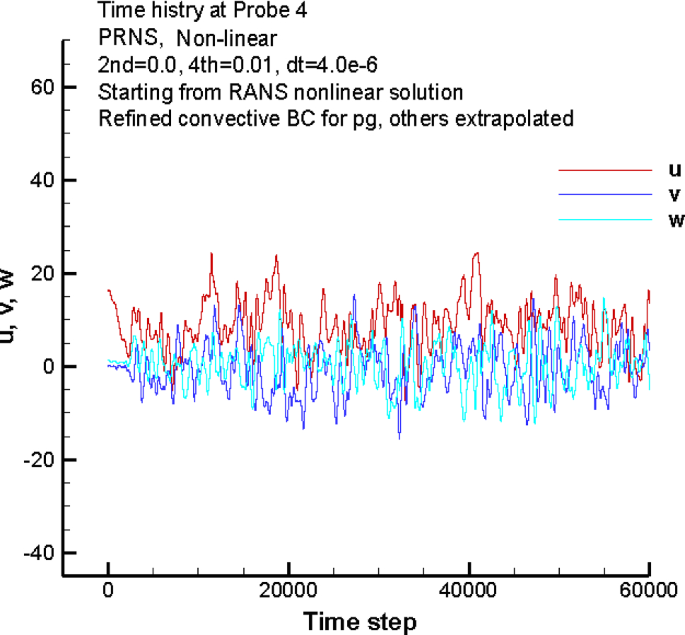
Turbulent flow is characterised by seemingly random fluctuations, and we can see these shown above for the three velocity components u, v, and w. We can see that the velocity is given in the so-called time domain, i.e. the x-axis is the time axis (here shown as time steps, which can be transformed into time by multiplying the time step with the time interval \Delta t between time steps).

To analyse this flow, it is common to transform this time domain into a frequency domain. We do that by applying the Fourier transform to the velocity signal. The x-axis will now show frequencies, and the y-axis will show energy at any given frequency. If this seems confusing, that’s because it is. The Fourier transform is probably one of the strangest concepts students have to learn, so if you feel uncomfortable with the subject, I have an excellent recommendation for you: have a look at the explanation of the Fourier transform by 3Blue1Brown. Excellent channel.

If we look at the velocity signal above, then we see that these fluctuations have an almost wave-like behaviour. In fact, it seems like we have a lot of different sine or cosine waves stacked on top of one another, all with different frequencies (seen by different distances on the x-axis between one oscillation) and magnitudes (seen by the absolute value on the y-axis). The Fourier transform simply allows us to get the frequency and magnitude information, and we then transform the magnitude into an energy, which makes more sense in a fluid dynamic sense.

If we carry out this Fourier transform to one of the velocity components, then we get the following plot (on the left) in the frequency domain (sometimes also called the Fourier space):

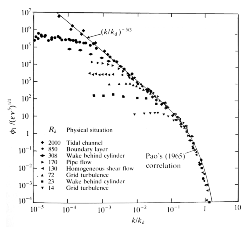
Look at the legend. We have channel flows, boundary layers, wakes, shear flow, and grid turbulence, all at different Reynolds numbers. Yet, all of these flows, in the frequency domain, collapse onto one and the same curve. Let’s look at the x-axis for a second. This isn’t actually given in frequencies f but rather in the so-called wave number k. We know from classical physics that we can compute a wave number from the frequency f as:

k=\frac{2\pi f}{u}

In this case, u is a velocity. But which one? If we look at the velocity component in the time domain, we see that the velocity is chaotic. We commonly make use of Taylor’s frozen turbulence assumption, which means that turbulence is, on a local scale, frozen, so that locally u can be regarded as some form of convective velocity, for example, the local mean velocity. With that information, we can express the frequency as a wave number.

Regardless of which unit we choose, all that will change are the values on the x-axis; the plot itself will remain exactly the same.

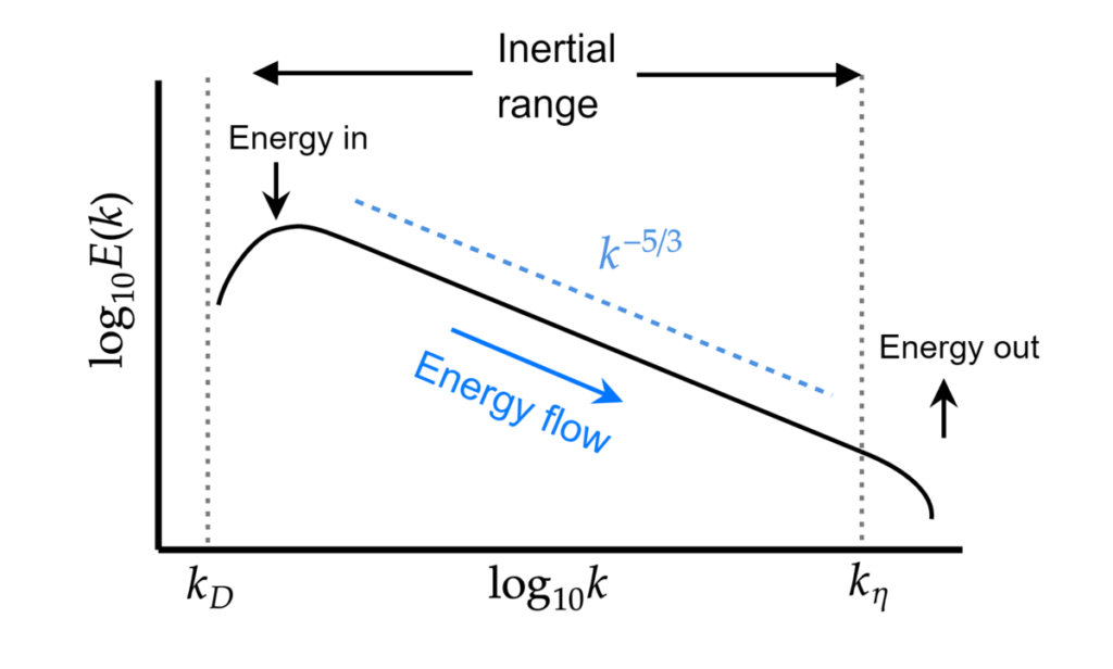
Kolmogorov now analysed different types of flows and realised that they all transferred their energy through the same mechanism. This is expressed as Kolmogorov’s famous k^{-5/3} law (or -5/3 in short). But what is meant by energy transfer here? Well, let’s look at the figure on the right. This shows schematically what is shown in the figure on the left.

Let’s introduce one more variable that will help us understand this plot: the eddy size. Turbulent flows consist of small, turbulent eddies that swirl around in our flow field. If we were to calculate a representative diameter (one that gives a circle with the same area as a turbulent eddy), then we can compute the characterisitc eddy size as l=2\phi /k. Thus, for small wave numbers (and frequencies, the eddy sizes have their largest value, while for high wave numbers, the eddy size is the smallest.

Now think about the vortex shedding behind a square cylinder as shown in the following video:

We can see large eddies forming just behind the square cylinder, as well as smaller eddies which are a result of the larger eddies (i.e. they will be generated by the larger eddies immediately behind the square cylinder forming in the wake). This is the key.

The largest eddies contain most of the energy (because of their size), but due to the friction of the fluid and rubbing (or shearing) against other eddies, they will lose their momentum over time. In order to retain their momentum, the eddies simply shrink whenever viscous shearing slows them down. If they shrink, l must become smaller (the characteristic size of the eddy), and since we have l=2\pi / k, or k=2\pi /l, as l reduces, k must increase.

In the figure above on the right, this means that we have to move to the right on the x-axis if k increases. Now, we also said that the y-axis represents energy. While eddies try to maintain their momentum, they constantly lose a bit of overall energy as they reduce in size (i.e. as they move to the right on the x-axis). We can see that the process of reducing eddy size while losing a bit of energy is universal, and all flows exhibit the same behaviour here. This is what Kolmogorov’s -5/3 law means in words.

Now that we understand that, we see that the energy for a turbulent flow is produced at the largest eddy sizes l (smallest wave numbers), as depicted by the figure on the right. You will very often hear the term “produced” in the context of turbulent flows, although we know, of course, energy can’t be produced; it can only change its form, in this case, from laminar to turbulent energy. However, this terminology is so ingrained in me that you probably will hear me use that terminology a few more times.

We can also see that the energy is “destroyed” at the smallest eddy sizes l (largest wave numbers of k). Again, the energy isn’t destroyed (it is dissipated into heat, in this case), but again, we, for some reason, like to use the terminology destroyed here.

Based on his observation about the energy transfer mechanism, Kolmogorov also computed the length, velocity, and time scales at which the flow dissipates into heat (i.e. what is the highest wave number, or smallest length scale in our flow). These are known as the Kolmogorov microscales, and they are given as:

• Kolmogorov length scale

\eta=\left(\frac{\nu^3}{\varepsilon}\right)^\frac{1}{4}

• Kolmogorov time scale

\tau_\eta=\sqrt{\frac{\nu}{\varepsilon}}

• Kolmogorov velocity scale

u_\eta = (\nu\varepsilon)^\frac{1}{4}

Here, \nu is the kinematic viscosity and \varepsilon the dissipation rate of the flow. Knowing these two quantities, we can compute what the smallest length, time, and velocity scales are in any given turbulent flow.

The dissipation can be computed directly from the gradient of the fluctuating velocity component. If we have that information available, then we can get that with a bit of data manipulation in a post-processing software like ParaView or Tecplot. If we don’t have the full turbulent field available, we can approximate the dissipation using the following approximations:

First, we calculate the Reynolds number:

Re=\frac{\rho U L}{\mu}

Next, we have to determine the turbulent intensity, which is the ratio of the (root mean square) velocity fluctuations to the mean velocity, i.e. I=u'_{rms}/\bar{u}, where \bar{u} is the mean velocity. For external aerodynamics in a wind tunnel, we may get values that are as low as I=0.0005. If we drive a car through the air, we may have I=0.01 on a calm day and I=0.1 on a windy day. For internal flows, we can approximate the turbulent intensity based on the Reynolds number as:

I=0.16 Re^{-1/8}

The turbulent intensity available, we can approximate the turbulent kinetic energy as:

k=\frac{3}{2}(UI)^2

Next, we compute the characteristic length scale (e.g. eddy size) in our flow. For external flows, we need to approximate the height of the boundary layer, and then we take 22% of the height of the boundary layer as an approximate eddy size, which we know to be representative for all eddies (in an average sense) from measurements.

Thus, we may have:

l=0.22\cdot\left(\frac{5L}{Re_L^{0.5}}\right),\quad \text{laminar, external flow (Re<2300)}\\[1em]
l=0.22\cdot\left(\frac{0.37L}{Re_L^{0.2}}\right),\quad \text{turbulent, external flow (Re>2300)}\\[1em]
l=0.038\cdot L_{\text{diameter}},\quad \text{internal flow, circular pipe}

With these values, we can approximate the dissipation rate as (with the coefficient C_\mu=0.09):

\varepsilon = C_\mu^\frac{3}{4} k^\frac{3}{2} l^{-1} 

Let’s see this in action for an example. We want to compute the Kolmogorov microscales for a pipe flow at a Reynolds number of Re=10,000. The pipe has a diameter of L_\text{Diameter}=D=10 cm=0.1m and the length of the pipe is L=1m. We assume water for our simulation with properties given at room temperature. Specifically, we have

• Density: \rho=998\, kg/m^3
• Viscosity: \mu=10^{-3}\, Pa\, s

We have the Reynolds number, so we can compute the characteristic velocity, turbulent intensity, turbulent kinetic energy, and characteristic length scale as:

U=\frac{Re\,\mu}{\rho D}=\frac{10,000\cdot10^{-3}}{998\cdot L}= 0.1 \frac{m}{s} \\[1em]
I=0.16 Re^{-1/8}=0.16\cdot10,000^{-1/8}=0.0506\\[1em]
k=\frac{3}{2}(UI)^2=\frac{3}{2}(0.01\cdot0.0506)^2=3.86\cdot 10^{-5}\frac{m^2}{s^2}\\[1em]
l=0.038\cdot D=0.038 \cdot 0.1=0.0038\, m

With that, we can approximate the dissipation rate to be:

\varepsilon = C_\mu^\frac{3}{4} k^\frac{3}{2} l^{-1} =0.09^\frac{3}{4}\cdot (3.86\cdot 10^{-5})^\frac{3}{2}\cdot 0.0038^{-1}\approx 10^{-5}\,\frac{m^2}{s^3}

With that, we can compute the Kolmogorov microscales as (using \nu=\mu/\rho=10^{-3}/998=10^{-6}

\eta=\left(\frac{\nu^3}{\varepsilon}\right)^\frac{1}{4}=\left(\frac{(10^{-6})^3}{10^{-5}}\right)^\frac{1}{4}=(10^{-13})^\frac{1}{4}=5.58\cdot 10^{-4}\, m=0.558\, mm\\[1em]
\tau_\eta=\sqrt{\frac{\nu}{\varepsilon}}=\sqrt{\frac{10^{-6}}{10^{-5}}}=\sqrt{10^{-1}}=0.3\, s \\[1em]
u_\eta = (\nu\varepsilon)^\frac{1}{4}= (10^{-6}\cdot 10^{-5})^\frac{1}{4}=(10^{-11})^\frac{1}{4}=1.79\cdot 10^{-3}\, s

Of particular importance here is the Kolmogorov length scale. It essentially tells us what the smallest mesh size should be in our domain, so that we capture all turbulence. If we assume that we want to resolve all turbulence with a structured grid, using a hexahedral element, then we can compute the volume of a single element as

V_{cell}=\Delta x\Delta y \Delta z=\eta\cdot\eta\cdot\eta =\eta^3=(5.58\cdot 10^{-4})^3=1.74\cdot 10^{-10}\,m^3

We can also compute the volume of the flow domain. We said we use the flow through a circular pipe with a length of 1 metre and a diameter of 10 centimetres (or 0.1 metres). This gives us a radius of r=0.05 metres. Thus, the volume of the pipe can be computed as:

V_{pipe}=A_{circle}\cdot L = 2\pi r^2\cdot L=2\pi\cdot0.05^2\cdot 1=1.57\cdot 10^{-2}\, m^3

To compute the number of cells we need to map the pipe volume with our hexahedral cells, we simply compute

\text{number of cells}=\mathrm{round}\left(\frac{V_{pipe}}{V_{cell}}\right)=\mathrm{round}\left(\frac{1.57\cdot 10^{-2}}{ 1.74\cdot 10^{-10}}\right)\approx 9,000,000

9 million cells isn’t too bad to resolve a turbulent flow. But if we now also consider the CFL number, then we can compute the time step. Typically, we want to advect the flow in time with a CFL number of one so that we have a good resolution in time. This means that our time step is:

CFL=u\frac{\Delta t}{\Delta x}\quad \rightarrow\quad \Delta t=\frac{CFL\cdot\Delta x}{u}=\frac{1\cdot5.58\cdot 10^{-4}}{0.1}=5.57\cdot10^{-3}\, s

This is much smaller than the time scale \tau_\eta=0.3\, s, which is quite common for turbulent flows, i.e. our CFL condition is typically giving us a time step that is smaller than the characteristic time scale in a turbulent flow. Therefore, we are more limited by the numerics than the physical processes here.

In order for the flow to pass through the pipe once, we need to compute the flow for L/(U\cdot \Delta t)=1800 time steps. So we solve the flow on our 9 million cell mesh 1800 times. This is still feasible with a good cluster, and we should be able to get results within a few hours if we have about 100 cores available.

But what happens if we increase the Reynolds number now to 100,000? In that case, we need now 8,400,000,000 cells, i.e. 8.4 billion cells, and we have to solve the flow here for at least 8120 time steps to get at least one pass of the flow through the pipe. And this is just for a pipe flow at a still moderate Reynolds number.

If we do the same calculation now for an aircraft (of the order of a Boeing 737 or an Airbus 320), cruising at 35,000 feet, then we need about 900 billion cells, and about 100,000 time steps to have the flow pass over the aircraft once. You can see how the computational resources quickly escalate, and so we stand no chance of resolving turbulence down to the smallest scales.

This means that we have to resort to modelling the effects of turbulence. And this is where the CFD literature offers us a plethora of different modelling strategies, all with varying degrees of complexity and grid requirements. In the remainder of this article, I want to shine a light on these different turbulence modelling approaches and show which can be used for what kind of flow simulation.

But before we look at the details of turbulence modelling, we need to look at two fundamental concepts in turbulence to understand the modelling requirements later. These are the boundary layer and the origin of turbulence (and how a flow transitions from a laminar to a turbulent flow). We will look at these, then at the modelling itself.

Turbulent boundary layers and the y+ value

When we deal with turbulent flows, turbulent boundary layers are by far the most computationally intensive aspect of our flow to resolve. Boundary layers are a thin layer that forms at solid walls. A schematic for them is given below:

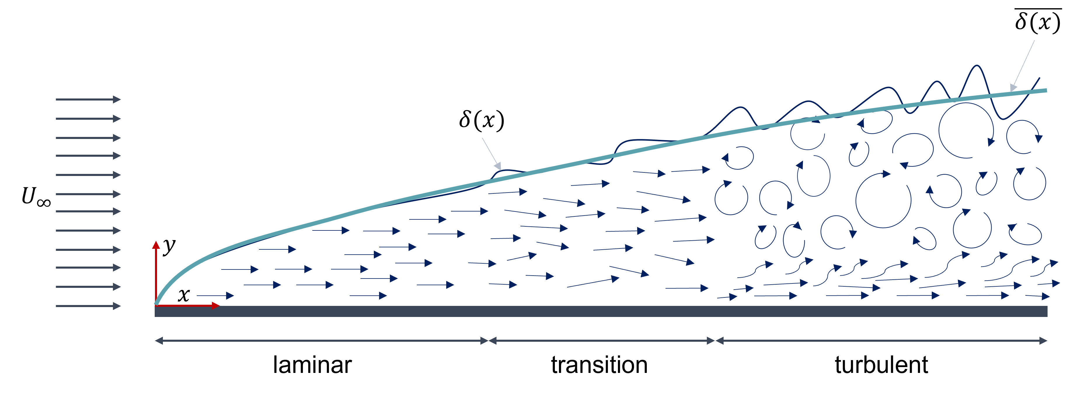
A boundary layer can be separated into 3 regions: a laminar, a transition, and a turbulent region. A laminar flow is one where the flow is well aligned, travels in one direction, and we have no mixing between fluid layers. Well, there is mixing, but it is proportional to the diffusion strength, and diffusion alone is usually a very weak mechanism for mixing. Think of a tea bag in still water; it will take time for the tea to diffuse out of the tea bag, but once you stir the water, you add (turbulent) convection, which is a much stronger mechanism for mixing.

Turbulence, then, as we have discussed above, is the opposite, where we have seemingly chaotic motion. Close to the wall, we still have some seemingly aligned flow, which is due to the velocity having to come to zero at the wall. If the velocity is close to zero, the flow will become essentially laminar again. In other words, viscosity dominates the flow here and damps any turbulent oscillation. The laminar and turbulent boundary layers are connected by a rather short region in which the flow is intermittent; it is neither fully laminar nor fully turbulent, but rather both regimes can exist here.

A while ago, I saw this excellent video on laminar vs. turbulent flows, which is highly recommended (and, for that matter, Veritasium in general):

We see a constant velocity profile arriving on the left of the boundary layer in the figure above. We have placed a solid wall at the origin of the x, y coordinate system. Once this velocity arrives at the wall, it starts to form a boundary layer immediately, and we can see that the height of the boundary layer is given by \delta (x,t). This is the instantaneous boundary layer height at a given location x and for a given point in time t. We can also compute the time-averaged boundary layer height, which is given by \bar{\delta x}(x).

Schlichting performed a lot of measurements on boundary layers and was able to publish an entire book about them, and from him, and measurements by others, we have empirical formulations that help us to determine the height of a boundary layer for both laminar and turbulent flows at any given location x. These are given as:

\overline{\delta(x)}_{laminar}=5\frac{x}{\sqrt{Re_x}}\\[1em]
\overline{\delta(x)}_{turbulent}=0.37\frac{x}{Re_x^{0.2}}

Here, the Reynolds number is defined as:

Re=\frac{\rho U x}{\mu}

where x is the location along the solid wall, and we define x=0 as the origin of the solid wall. That is, the Reynolds number is zero here and then increases monotonically.

If we look at the boundary layer above again, then we can see that there are three distinct regions, i.e. the laminar, the transition, and the turbulent regions, but we can also see that there are three separate regions with a turbulent boundary layer. We already discussed the viscous region close to the wall, where the flow turns locally to an essentially laminar flow. But what happens further away from the wall? The velocity reaches almost free-stream conditions, and so we have enhanced turbulent mixing here.

Since we said that there is a transition region between laminar and turbulent flows, it stands to reason that there ought to be a transition region between the viscous and enhanced turbulent mixing regions. If we wanted to investigate that for different boundary layer flows, though, we would get different thicknesses for each of these regions. If I wanted to go into the wind tunnel and take a measurement at 3mm away from the wall, I would have no idea if that is in the viscous, transition, or enhanced turbulent mixing region.

Thus, whenever we can, we like to generalise concepts, and so we attempt now to scale boundary layers so that they all look one and the same. If we have achieved that, then we can go into this general boundary layer, specify what region we are interested in, and then scale it back to the original boundary layer. This would give us the location in physical space.

Whenever we want to collapse curves or functions onto the same space, we typically resort to non-dimensionalisation, and this is what scientists did with turbulent boundary layers as well, and, as it turns out, this non-dimensionalisation is extremely useful for us as CFD practitioners, as it will help us during mesh generation to determine how much of the boundary layer we want to resolve by specifying the height of our cells in the boundary layer region.

So, how do we go about normalising the boundary layer? Well, we need to figure out which quantity exists that naturally scales with the height of the boundary layer. Take a look at the following figure for two separate boundary layer flows:

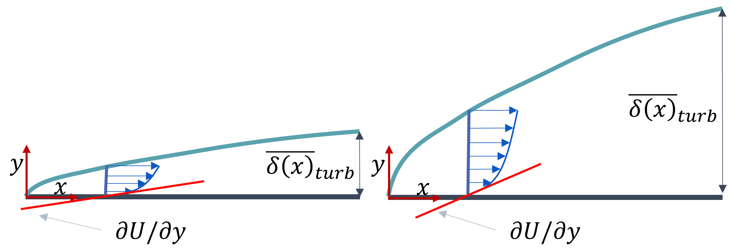
The boundary layer on the left is much smaller than that on the right, but in both cases, the velocity gradient at the wall, in the wall normal direction (here, the y-axis), does scale with the height of the boundary layer. So, the velocity gradient presents a natural choice to scale the height of the boundary layer. In the literature about turbulent flows, the wall normal direction is always the y-axis. If the boundary is curved, then we need to use a different definition, but the literature is typically only concerned with flat plates and the like.

Then, you may remember that Newton’s law of viscosity states that the shear stresses (in this case, at the wall) are related to the velocity gradient as:

\tau_w=\rho\nu\frac{\partial U}{\partial y}

Let’s write the density on the left-hand side, and we get:

\frac{\tau_w}{\rho}=\nu\frac{\partial U}{\partial y}=\left[\frac{m^2}{s^2}\right]

We can see that from a purely dimensional ground, both sides have units of a squared velocity, i.e. m^2/s^2. So, if we now take the square root of the left-hand side, for example, we have:

u_*=\sqrt{\frac{\tau_w}{\rho}}=\left[\frac{m}{s}\right]

In this context, u_* is the so-called friction velocity, and it gets its name from the wall shear stresses, which can be thought of as a friction force of some form. Thus, we can say that this friction velocity is a representative velocity for different boundary layers, and it will grow larger as our boundary layers grow larger. Therefore, we can now introduce a non-dimensional coordinate axis as:

y^+=y\cdot\frac{u_*}{\nu}

Here, we multiply the local coordinate axis in the y direction by the friction velocity. This gives us units of m^2/s. The kinematic viscosity has the same units, so by dividing by this viscosity, we arrive at a non-dimensional coordinate direction. Since the turbulent literature always considers the y-axis to be the wall normal direction, we call this new non-dimensional coordinate direction the y^+ (y plus) coordinate.

We can also non-dimensionalise our velocity. Since we have defined the friction velocity already, we can simply divide the instantaneous velocity by this friction velocity, which will give us:

u^+=\frac{U}{u_*}

In analogy to the y^+ value, we call this non-dimensional velocity the u^+ (u plus) velocity component. Now, we can plot any turbulent boundary layer flow inside a y^+ vs u^+ plot, and the result of doing that is shown in the figure below on the left.

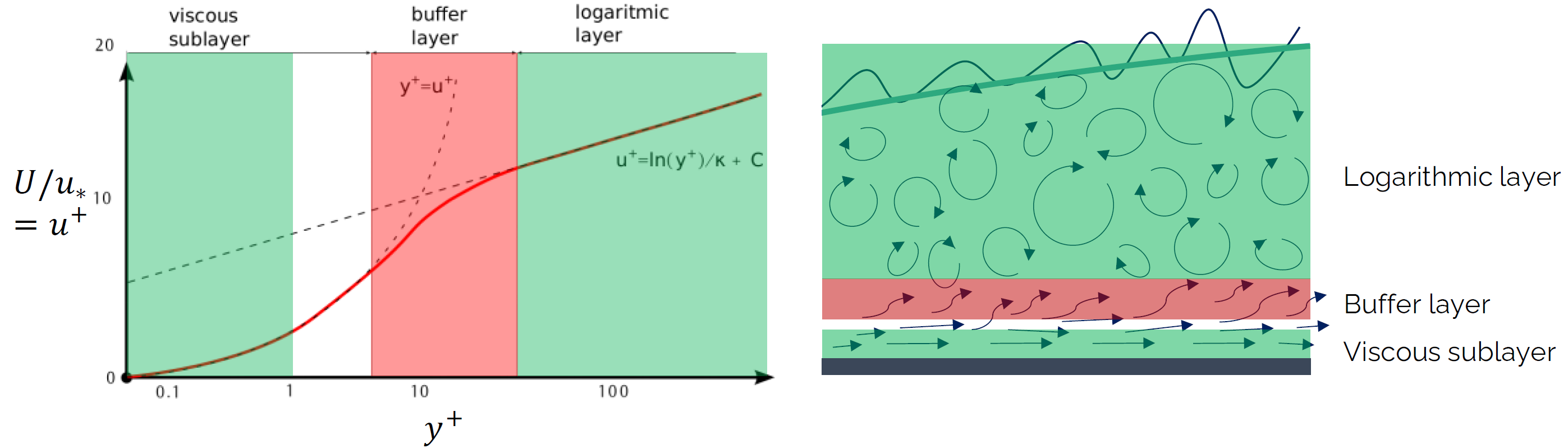
Regardless of which turbulent boundary layer you take, or at which position you measure the flow, you will always get the plot that you see in the figure above on the left. It might get shifted up or down a bit, typically based on surface roughness, but the shape of the curve will remain the same. This is such a fundamental finding in turbulent boundary layer flows that this has become known as the law of the wall.

Let’s investigate the plot a bit. First of all, the plot is given with a logarithmic x-axis and a linear y-axis. This just helps us to better see what is happening to our velocity profile. As we go to the left on the x-axis, we approach the wall, and as we go to the right, we move away from the wall. We can see the two separate regions I mentioned before; the viscous region close to the wall is known as the viscous sublayer, while the enhanced turbulent mixing region is known as the logarithmic layer. The transition region in between is known as the buffer layer.

We see a fundamental change in the velocity profile as we transition away from the wall. Initially, the velocity profile follows the relation u^+=y^+. Since this is a semi-logarithmic plot, any linear relation will appear as an exponential function. We see that this behaviour holds true for y-plus values up to y^+\approx 5. Thus, we can say that the viscous sublayer is located between 0\le y^+ < 5.

In the logarithmic layer, we see that we have a, well, logarithmic relationship which is given as u^+=\ln(y^+)/\kappa + C. Again, since the plot uses semi-logarithmic axes, a logarithmic profile will appear as a straight line. Here, \kappa=0.41 is the von Karman constant and C=5.0, both obtained from measurements in experiments.

In between these two regions, we said that there exists a buffer layer, and the velocity profiles change from linear to logarithmic here. This buffer region is typically located at 5 \le y^+ < 30, and the logarithm region is typically located between 30 \le y^+ < 0.3\cdot y/\bar{\delta}(x), where y and \bar{\delta}(x) are the dimensional y-axis and boundary layer height, respectively.

In the figure above on the right, we see how these regions map to the physical representation of the boundary layer. We have the viscous sublayer close to the wall, where the velocity profile will be linear. Then, we transition through the buffer layer to the logarithmic layer.

When we deal with turbulence modelling in CFD, as alluded to above, most of the complexity (and computational cost) will come from resolving (or modelling) the flow near solid boundaries with turbulent boundary layers. Since these regions are so thin, if we can effectively model them, then there is no need to resolve them completely, and we can save grid cells in this region, and, by extension, reduce the computational cost significantly.

Most of the turbulence modelling approaches that we will discuss in the next articles and that were introduced over the years had the same motivation: to model as much turbulence as possible to reduce the computational cost without affecting accuracy too much. As a result, for different applications, different turbulence modelling approaches were introduced, and it is down to us now to figure out which modelling approach works best for us. We will look at the most commonly used turbulence modelling approaches in this article. But first, let us look at how turbulence is generated in the next section.

The origin of turbulence

We now have an understanding of the scales of turbulence, and we also looked at boundary layer flows. What I want to do in this section is to look at the origins of turbulence and see, both in a physical and mathematical sense, how turbulence is generated.

How is turbulence generated in a physical sense?

We start our discussion with how turbulence is generated in a physical sense. First of all, we assume that our flow is laminar, i.e. we have a well-aligned flow. This flow transitions into a chaotic, turbulent flow through various mechanisms. There are 4 main transition mechanisms which we will look at below in order.

Natural transition

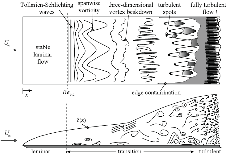
As the velocity increases, the non-linear term will start to introduce small fluctuations. These fluctuations then feed into the so-called Tollmien-Schlichting waves, which grow alongside the flow within a laminar boundary layer.

As these waves grow, they break down and form even larger structures, which eventually become so powerful that they locally transition into turbulence. Once enough turbulent spots are generated, they will transition the entire boundary layer into a fully turbulent flow.

Natural transition requires a low freestream turbulent intensity.

Bypass transition

Bypass transition, on the other hand, has a higher freestream turbulent intensity, and it bypasses the various waves that are generated by natural transition. It does so by feeding higher turbulent intensity from the freestream (i.e. fluctuations/perturbations) directly into the laminar boundary layer.

These fluctuations then cause the laminar boundary layer to produce turbulent spots, but because the boundary layer does not have enough energy to transition into turbulence, these turbulent spots will be much longer compared to those occurring in natural transition.

Separation-induced transition

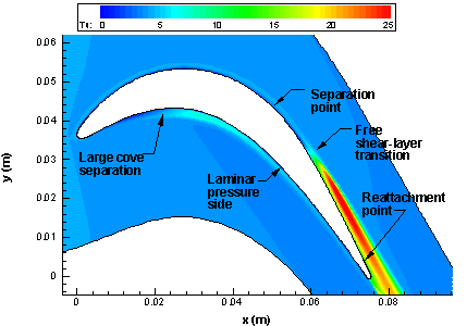
Separation-induced transition occurs in cases where the flow separates from the wall, at a point where the flow is still laminar. When the flow is separated, it is no longer confined to move along the wall, and this additional flexibility in movement, together with the freestream that may feed some turbulent intensity into the separated flow, will cause the transition from laminar to turbulence.

The example on the left shows how flow separates in an adverse pressure gradient (adverse = pressure is reducing), which can be found in turbine sections on an engine.

Crossflow transition

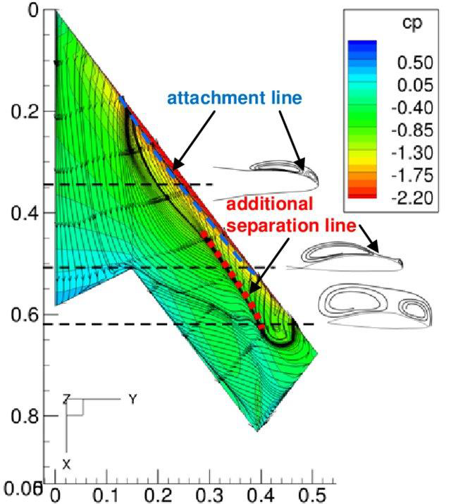
Crossflow transition happens in cases where the main flow is laminar, but it gets injected from the streamwise direction with additional velocity (i.e. with crossflow).

The example on the left shows this for a delta wing, where the flow is coming from the top and is going to the bottom. At three different sections, we cut through the geometry and can see the flow structure to the right.

Due to the pressure difference (lower pressure on the top, higher pressure on the bottom), the flow will move from the high-pressure region (bottom) to the low-pressure region (top). The flow has to move around the leading edge, and due to the geometry of the leading edge, there will be a crossflow component in the velocity.

This will be injected into the main flow and act as a disturbance, which pushes the main flow sideways and in the process triggers transition to turbulence in the boundary layer.

How is turbulence generated in a mathematical sense?

We will now look at the mathematics of turbulence, but we will keep it at a very simple level. Turbulence is full of complicated integral and differential equations. My goal isn’t to reproduce what the literature is already providing us in abundance, instead, I want to focus in on the essentials. A bit of math is required, but it isn’t that complicated.

We already looked at the behaviour of the velocity above, let us now formally introduce that by looking at the figure below:

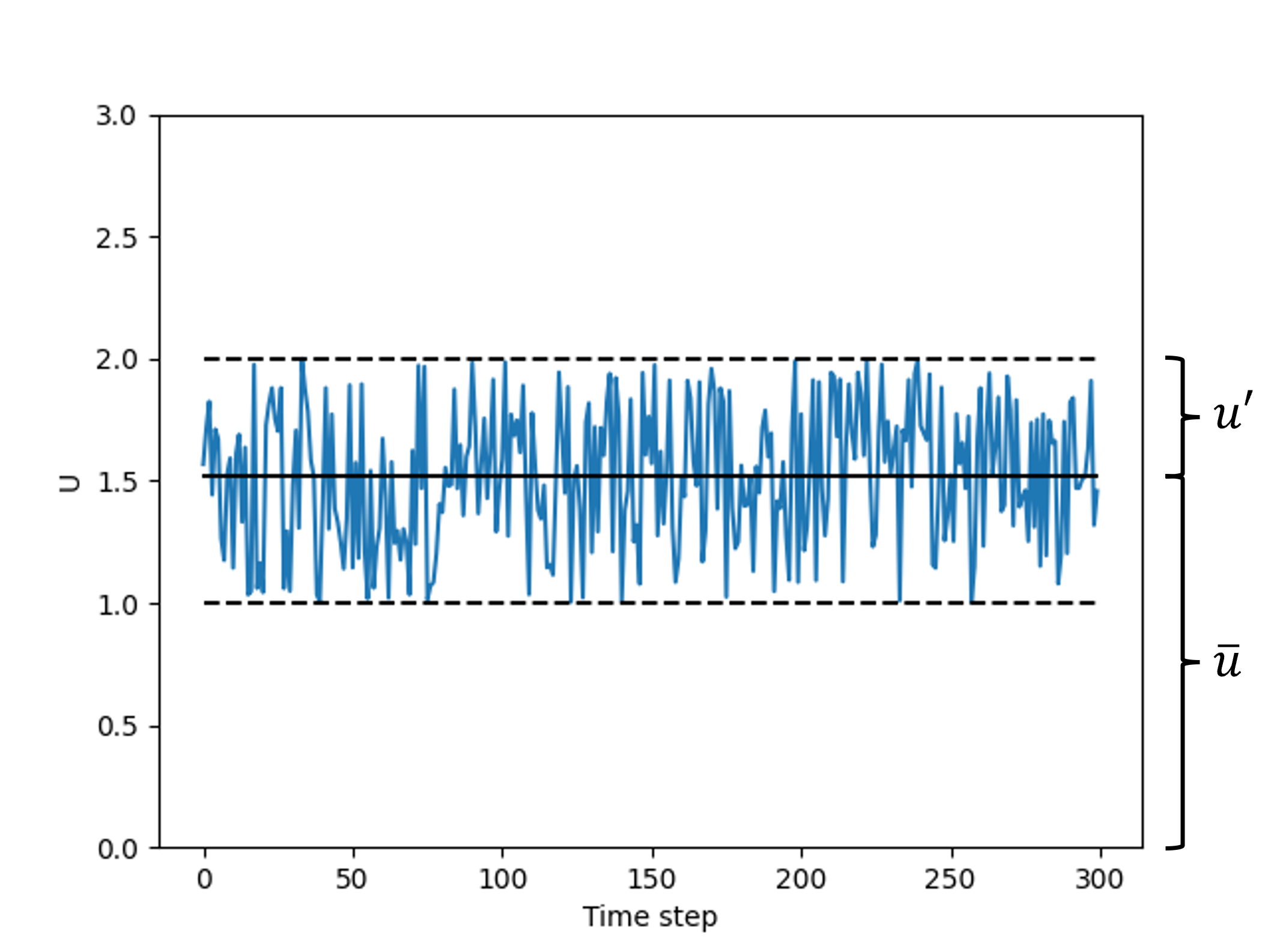
We see here a velocity signal that is seemingly random, but there is a way for us to decompose this signal into something meaningful. We can see that the fluctuations are all centred around a mean value of the velocity, which we will call \bar{\mathbf{u}}. Then, the velocity fluctuations, denoted as \mathbf{u}', are simply oscillating (fluctuating) around this mean value. This is shown on the right of the figure, and we can express the instantaneous velocity (the absolute velocity component) at any given time as:

\underbrace{\mathbf{U}}_\text{instantaneous}=\underbrace{\bar{\mathbf{u}}}_\text{mean} + \underbrace{\mathbf{u'}}_\text{fluctuation}

This is the most complicated mathematical concept you will have to understand in this section. See, I promised it wouldn’t get too complicated. At the same time, it is also one of the most fundamental concepts. The velocity decomposition above is known as the Reynolds decomposition, as introduced by Osborne Reynolds. It is a vital concept in the theory of turbulence, and we will see this velocity decomposition quite a few times in the rest of this article.

If we decompose the instantaneous velocity into its mean and fluctuating part, then we can define some properties. The first one is that of the mean quantity, which can be expressed as:

\bar{\phi}=\frac{1}{T}\int_0^T\phi(t)\mathrm{d}t

If we have a time series of \phi, for example, \phi=(1, 2, 3), then we can compute the discrete integral above by adding the product of each sample with the time step and dividing by the total time. If we set the time step \Delta t=0.1 seconds, then we have (\Delta t/T)\cdot (1 + 2 + 3)=(0.1/0.3)\cdot (6)=(1/3)\cdot 6 = 2. If we look at the original time series, i.e. \phi=(1, 2, 3), we could have probably guessed that the average ought to be 2 (assuming a constant time step), the above is just the formal mathematical description.

For the fluctuation velocity component, which we can also express as \mathbf{u}'=\mathbf{U}-\bar{\mathbf{u}}, we can reason from the figure above that if we subtract the mean from the instantaneous velocity component, that the integral (average) of the remaining fluctuating component must be zero, as it is oscillating (fluctuating) around zero velocity. This can be expressed in mathematical form as:

\frac{1}{T}\int_0^T\phi'(t)\mathrm{d}t=0

With these two definitions and the decomposition of the velocity into a mean and fluctuating velocity component, we are ready to apply our knowledge to the Navier-Stokes equations. Let’s use the momentum equation for an incompressible flow with instantaneous values. We do that by capitalising the velocity and pressure components. Then we have:

\frac{\partial \mathbf{U}}{\partial t} + (\mathbf{U}\cdot \nabla)\mathbf{U}=-\frac{1}{\rho}\nabla P+ \nu \nabla^2 \mathbf{U}

To make the discussion easier, we will just consider a one-dimensional fluid. This will make the mathematical description a bit easier to follow, though I should stress again that turbulence is a three-dimensional effect. The momentum equation in one dimension is written as:

\frac{\partial U}{\partial t}+ U\frac{\partial U}{\partial x}=-\frac{1}{\rho}\frac{\partial P}{\partial x} + \nu\frac{\partial^2 U}{\partial x^2}

This equation is written in non-conservative form. For an incompressible flow, we saw in my last article, where we discussed the difference between primitive and conserved variables, that due to the incompressible continuity equation, i.e. \nabla\cdot\mathbf{u}=0, both the conservative and non-conservative formulations are mathematically equivalent. Therefore, let’s write the equation in conservative form:

\frac{\partial U}{\partial t}+ \frac{\partial UU}{\partial x}=-\frac{1}{\rho}\frac{\partial P}{\partial x} + \nu\frac{\partial^2 U}{\partial x^2}

Now we introduce Reynolds’ velocity decomposition for the instantaneous velocity and pressure. This is given as:

\frac{\partial (\bar{u}+u')}{\partial t}+ \frac{\partial (\bar{u}+u')(\bar{u}+u')}{\partial x}=-\frac{1}{\rho}\frac{\partial (\bar{p}+p')}{\partial x} + \nu\frac{\partial^2 (\bar{u}+u')}{\partial x^2}

The equation above is exact, i.e. it fully describes a turbulent flow. The only complication is that we have to deal with time-averaged and non-time-averaged components. If we want to extract some meaning from these equations, i.e. will be easier if we average these equations in time. Then, we can see how turbulence is represented in terms of mean flow quantities. So let us do just that.

We will now attempt to time-average the above-shown momentum equation. This can be written as:

\frac{\partial \overline{(\bar{u}+u')}}{\partial t}+ \frac{\partial \overline{(\bar{u}+u')(\bar{u}+u')}}{\partial x}=-\frac{1}{\rho}\frac{\partial \overline{(\bar{p}+p')}}{\partial x} + \nu\frac{\partial^2 \overline{(\bar{u}+u')}}{\partial x^2}

Let’s see how we can evaluate the time average for these components. Let’s start with the linear terms. Here, we see that we either have to deal with the velocity or the pressure component. The time averages can be written as:

\overline{(\bar{u}+u')}=\underbrace{\overline{\bar{u}}}_{=\bar{u}}+\underbrace{\overline{u'}}_{=0}=\bar{u}+0=\bar{u}\\[1em]
\overline{(\bar{p}+p')}=\underbrace{\overline{\bar{p}}}_{=\bar{p}}+\underbrace{\overline{p'}}_{=0}=\bar{p}+0=\bar{p}

We see that we can decompose the time averages and take the time averages of the mean and fluctuating parts independently. If we take an average or an already averaged quantity, we will simply get the average back. So the average of the average velocity and pressure is just the average velocity and pressure. Nothing has changed here. But we saw above that if we take the time average of a fluctuating component, then by definition, this time average has to be exactly zero. That is just the definition of the fluctuating velocity component.

Since the fluctuating component goes to zero when time-averaged, this means that taking the time average of any linear term, containing either the velocity or pressure, will just return the time-averaged component of either the velocity or pressure. So nothing changes for the linear terms. But let’s have a look at the non-linear term. Here, we have:

\overline{(\bar{u}+u')}\overline{(\bar{u}+u')}=\underbrace{\overline{\bar{u}\bar{u}}}_{=\bar{u}\bar{u}}+\underbrace{\overline{\bar{u}u'}}_{=\bar{u}\cdot 0=0} +\underbrace{\overline{u'\bar{u}}}_{0\cdot \bar{u}=0} +\underbrace{\overline{u'u'}}_{\ne 0}

We have to multiply the parentheses, which gives us four products. The first is that of two mean velocities. These are already time-averaged. If we take the time average of this component again, we simply get back the time average. For the second and third terms, we multiply the time-averaged velocity by the fluctuating velocity component. Since we take the time average, which is zero for the fluctuating velocity component, both the second and third terms are a multiplication of a mean velocity by zero, and thus this product has to be zero.

But for the fourth and last term, the picture isn’t as clear. Here, we say that if we multiply the fluctuating velocity component with itself (or. for that matter, with any other fluctuating velocity component if we are in three-dimensional space), this product is not equal to zero. Why is that? We just said that terms 2 and 3 are zero because we take the time average of the fluctuating velocity, which is zero, so why is the fourth term then not a product of zero times zero?

The answer is that velocity fluctuations are correlated. For an uncorrelated signal, that is, if you take the time-average of two randomly generated time series, then you do get a value of zero. But, for a correlated signal, we get a non-zero value. While we could show this with equations, let’s make this a bit more intuitive. Let us generate two random time series and compute their time averages, and then repeat this for three correlated signals and see how they compare.

First, we create two random time series. Let’s call these u and v. Then, let’s introduce three correlated signals, which we call v1, v2, and v3, which all depend on the randomly generated time series of u. Specifically, let’s consider the following correlation (or, functional relationship, both mean the same thing):

• v1: f_{v1}(u)=0.7\cdot u
• v2: f_{v2}(u)=\sin(u)
• v3: f_{v3}(u)=-(\mathrm{d}u/\mathrm{d}t)

Here, v1 is just a scaled version of u, while v2 is taking the sine of u. With v3, we are doing something slightly different in that we take the negative derivative of u. What we want to see is how the correlation changes as we use more and more samples. The code below implements these in Python:

import numpy as np
import matplotlib.pyplot as plt

number_of_samples = [10, 100, 1000, 10000, 100000, 1000000, 10000000]

random_mean_list = list()
for sample in number_of_samples:
    # generate two random time series which are no correlated
    random_u = np.random.uniform(-1, 1, sample)
    random_v = np.random.uniform(-1, 1, sample)

    # calculate product of u'v'
    random_mean = 0
    for i in range(0, sample):
        random_mean = random_mean + random_u[i] * random_v[i]
    random_mean = random_mean / sample

    random_mean_list.append(random_mean)

correlated_mean_1_list = list()
correlated_mean_2_list = list()
correlated_mean_3_list = list()
for sample in number_of_samples:
    # generate three correlated time series
    correlated_u = np.random.uniform(-1, 1, sample)
    correlated_v1 = correlated_u * 0.7
    correlated_v2 = np.sin(correlated_u)
    correlated_v3 = np.zeros(sample)
    for i in range(0, sample - 1):
        correlated_v3[i] = - (correlated_u[i + 1] - correlated_u[i]) 

    # calculate the correlation coefficient between time series u'v1', u'v2, and u'v3'
    correlated_mean_1 = 0
    correlated_mean_2 = 0
    correlated_mean_3 = 0
    for i in range(0, sample):
        correlated_mean_1 = correlated_mean_1 + correlated_u[i] * correlated_v1[i]
        correlated_mean_2 = correlated_mean_2 + correlated_u[i] * correlated_v2[i]
        correlated_mean_3 = correlated_mean_3 + correlated_u[i] * correlated_v3[i]
    correlated_mean_1 = correlated_mean_1 / sample
    correlated_mean_2 = correlated_mean_2 / sample
    correlated_mean_3 = correlated_mean_3 / sample

    correlated_mean_1_list.append(correlated_mean_1)
    correlated_mean_2_list.append(correlated_mean_2)
    correlated_mean_3_list.append(correlated_mean_3)

# plot the correlations vs. sample size
plt.semilogx(number_of_samples, random_mean_list, label='random')
plt.semilogx(number_of_samples, correlated_mean_1_list, label='correlation 1')
plt.semilogx(number_of_samples, correlated_mean_2_list, label='correlation 2')
plt.semilogx(number_of_samples, correlated_mean_3_list, label='correlation 3')
plt.legend()
plt.xlabel('Number of samples')
plt.ylabel('time averaged correlation')
plt.show()

On line 4, we specify the number of samples we want to test. There are a few, and we want to see how the behaviour changes as we increase the sample size. Then, we go on to create two random time series u and v on lines 6-18, where we compute the product u*v. We repeat the steps here on lines 20-46, where we compute the correlations between u*v1, u*v2, and u*v3.

On line 30, we compute f_{v3}(u)=-(\mathrm{d}u/\mathrm{d}x). In this case, we assume samples to be separated by 1 unit, e.g. \Delta t=1. Therefore, when we write out the discretised form, e.g. -(\mathrm{d}u/\mathrm{d}x)\approx -(u^{n+1}-u^n)/\Delta t, since we divide here by \Delta t=1, we can remove the division and our equation turns into a simple difference equation.

On lines 49-56, we plot the results, and the result is shown below:

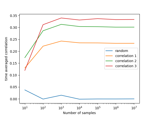
I have used a logarithmic scale here on the x-axis to see what is happening at low sample sizes. What we can take out of this plot is that as the sample size grows, the two random time series show no correlation, and their product u*v is zero. But all three correlated signals, i.e. u*v1, u*v2, and u*v3, do show a very non-zero correlation product.

Thus, to bring this discussion back to turbulence, why is the product of fluctuating velocity components correlated and how? Well, let’s consider for a moment a two-dimensional case. The continuity equation for the instantaneous velocity can be written as:

\nabla\cdot\mathbf{U}=\frac{\partial U}{\partial x} + \frac{\partial V}{\partial y}=\frac{\partial (\bar{u}+u')}{\partial x}+\frac{\partial (\bar{v} + v')}{\partial y}=\frac{\partial \bar{u}}{\partial x} + \frac{\partial u'}{\partial x}+ \frac{\partial \bar{v}}{\partial y}+\frac{\partial v'}{\partial y}=0

We see that we can also insert the Reynolds decomposition and then expand the derivatives. Let us split now the mean and fluctuating velocity component so that each appears on one side of the equation. Then we get:

\frac{\partial v'}{\partial y} + \frac{\partial u'}{\partial x} = -\frac{\partial \bar{u}}{\partial x} - \frac{\partial \bar{v}}{\partial y}

For a fully developed flow, for example, for the flow over an airfoil, the mean flow gradients will eventually converge to one value, but the fluctuating velocity component will never converge. These will always oscillate, and that is also the reason why your RANS simulations will have trouble converging even if you try to solve them as a steady state problem. Some fluctuations will always exist, and depending on their strength, you will not get your simulations to converge below a certain convergence threshold.

If our mean flow quantities and their gradients have converged, then we can also write the above equation as:

\frac{\partial v'}{\partial y} + \frac{\partial u'}{\partial x} = \text{constant}

In other words, the right-hand side will always be a constant. Therefore, if we have a change in u', then its gradient will also have to change. If the gradient of u' changes, then the equation above tells us that the gradient of v' has to change as well, and, as a result, v' changes as well. So, both u' and v' are correlated through the continuity equation, and as a result, the product of fluctuating velocity components is always correlated!

Let us now finish writing our equation. If we insert now the time averages for our Reynolds decomposed gradients, we get:

\frac{\partial \overline{(\bar{u}+u')}}{\partial t}+ \frac{\partial \overline{(\bar{u}+u')(\bar{u}+u')}}{\partial x}=-\frac{1}{\rho}\frac{\partial \overline{(\bar{p}+p')}}{\partial x} + \nu\frac{\partial^2 \overline{(\bar{u}+u')}}{\partial x^2}\\[1em]

\frac{\partial \bar{u}}{\partial t}+ \frac{\partial \bar{u}\bar{u}}{\partial x}+\frac{\partial \overline{u'u'}}{\partial x}=-\frac{1}{\rho}\frac{\partial \bar{p}}{\partial x} + \nu\frac{\partial^2 \bar{u}}{\partial x^2}

The above equation represents the time-averaged form of the momentum equation decomposed into its mean and fluctuation pressure and velocity components. The non-linear term produced an additional term, i.e. \partial (u'u')/\partial x, which we call the Reynolds stresses, or the Reynolds stress tensor (in two or three dimension, we will get a 2 by 2, and a 3 by 3 tensor, respectively).

We know that the Reynolds stress tensor is constructed of velocity fluctuations, which, by definition, are only present for a turbulent flow (for a laminar flow, u'=0). Therefore, we can say that the Reynolds stresses are an indicator of the level of turbulence in our flow. We also know that the Reynolds stresses were produced by time averaging the non-linear term. This means that it is the non-linear term that produces turbulence, in a mathematical sense.

Let’s bring that back to the schematic figure we saw above, which I have reproduced below:

We say that at low wave numbers (to the left on the x-axis), we have some energy input that is feeding the energy cascade, i.e. turbulence. This energy is coming from the non-linear term, which produces the Reynolds stresses, and it is these Reynolds stresses that produce turbulence at the lowest wave numbers (largest eddy sizes). Energy is then cascaded down to the highest wave numbers (smallest eddy sizes) where all turbulence is eventually destroyed through viscous heating.

This means that the energy is taken out of a turbulent flow at the smallest length scales through the dissipative term in the Navier-Stokes equation, i.e. \nu\nabla^2\mathbf{U}. An interesting problem starts to occur when we use a mesh that can not resolve the smallest length scales (which is commonly the case). In this case, we have an imbalance between the energy produced at the largest eddy sizes through the non-linear term and the energy destroyed at the smallest eddy sizes through the dissipative term.

How can we fix that? Well, I have written an entire blog post about it, so why spoil it? Feel free to read the section on turbulence modelling, it also discusses the velocity correlation and why it is not zero again from a different perspective (using experimental evidence). In a nutshell, we need numerical dissipation to recover some of the physical dissipation we lost by making our grid larger than the smallest scales in the flow.

This also explains why the central scheme, which we have looked at now in a few articles, can’t be used to approximate the non-linear term in the Navier-Stokes equation; it is just not dissipative enough! If we do resolve all turbulent flow scales, then the central scheme can be used again for the non-linear term, and sometimes we do exactly that (though we can still make use of high-resolution schemes, and people also do that).

So, to summarise, in a mathematical sense, we can see by time-averaging the Navier-Stokes momentum equation that turbulence is produced by the non-linear term. The time averaging produces a new term that we have labelled the Reynolds stresses. Since the Reynolds stresses are correlated through the continuity equation, we know that the Reynolds stresses are non-zero.

Furthermore, since we have to conserve momentum, if we generate more turbulence, i.e. we increase the magnitude of the Reynolds stresses, our mean flow gradients of the non-linear term have to reduce, as energy is taken away from them and fed into the Reynolds stresses. Momentum is conserved, which means that the sum of the mean flow gradient of the non-linear term and the Reynolds stresses has to stay constant (as both are coming from the non-linear term).

This is where turbulence is coming from, and it just highlights once more the importance of capturing this term accurately through our numerical schemes!

How is turbulence modelled in CFD?

We now have a good idea of what turbulence is and how it is generated. But that is just the starting point. Now we need to examine how we can model turbulence, and we have different approaches available to us. In general, these turbulence modelling approaches will trade resolution for computational cost; the more turbulence we want to resolve, the more computational power we need to use.

There are three main types of turbulence modelling that we will look at in the following, including derivatives of each of these methods. These are:

• Direct Numerical Simulations (DNS)
• Large Eddy Simulations (LES)
• Reynolds-averaged Navier-Stokes (RANS)

In DNS, we resolve all length scales of turbulence. We saw in our back-of-the-envelope calculation above that this quickly escalates in computational cost. We saw that increasing the Reynolds number quickly increased the number of cells required to resolve the flow.

In LES, we say that we no longer want to resolve the entire turbulent spectrum. We are happy to only focus on the largest energy-containing eddies and model the smallest eddies with a so-called sub-grid scale (SGS) model. We do that by making our mesh coarser compared to DNSs, which means we can no longer capture the smallest eddies (hence the need to model them with the SGS model).

In RANS, we say we don’t want to resolve any turbulence at all! The entire turbulent spectrum is modelled, which means that we have no restriction on the mesh size, and we can make our meshes as coarse as we want in order to save computational cost.

The comparison between DNS, LES, and RANS is shown in the following picture in terms of how much they resolve the turbulent energy spectrum:

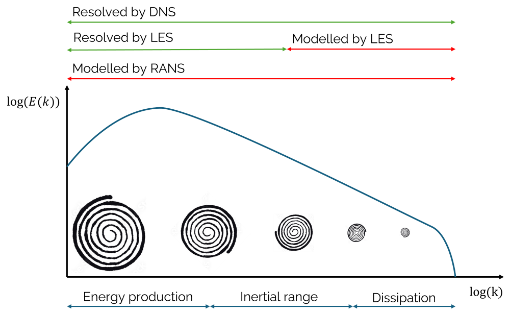
We can see here the turbulent energy spectrum again, and I have also given here some eddies within the plot to show that these are continuously decreasing as we increase the wave number k (which means we decrease the turbulent length scale l).

I have also given the names for the three regions in this turbulent spectrum plot, which are the energy production region for low wave numbers, the inertial range, and the dissipation region at the highest wave numbers. It is within this inertial range that we observe Kolmogorov’s k^{-5/3} law.

We can see from the figure above that DNS models the entire spectrum. The energy production (through the non-linear term, where mean flow gradients transfer some of their energy to the Reynolds stresses) is captured, and the turbulent energy is cascaded down to smaller eddies, until all eddies dissipate into heat. This happens when the local Reynolds number, based on the flow’s viscosity, the diameter of the eddy as a characteristic length, and the velocity based on the angular velocity of the eddy, reaches a value of 1, i.e. when viscosity starts to dominate.

LES, on the other hand, resolves only about 80% of the turbulent energy spectrum. How much is actually resolved depends on the mesh. If the mesh is too coarse, we may resolve less than 80%; if it is too fine, it is more, and we approach the resolution of DNS. A good simulation using LES as the turbulence modelling strategy aims for 80%, and we need to approximate the grid size here, typically by performing a RANS simulation first and using its values to compute the required grid size.

RANS does not capture any turbulence, and instead, models the entire spectrum. As alluded to above, this leads to significant cost savings in terms of computational cost, but it may also result in significant drawbacks, both in terms of modelling accuracy and capabilities, that make RANS fairly limited. Yet, it is the most common turbulence modelling approach that we use, not because of its modelling superiority, but out of necessity.

And then we have hybrid approaches, where we try to model turbulence as a mix of RANS and LES. We use RANS in the boundary layer to relax the rather strict grid requirements that are typically associated with LES, while keeping LES resolution in the farfield. This results in far fewer cells required, while still giving LES-like resolution. There are two main modelling approaches here, which go under the names of Detached Eddy Simulations (DES) and Scale Adaptive Simulations (SAS), although it is fair to say that DES seems to have won the race here; SAS is rarely used these days.

And then, we can also improve upon the accuracy of RANS by incorporating transitional effects, i.e. switching from laminar to turbulent flow. All RANS models, as we will see, are considered to simulate fully turbulent flow, which can sometimes give spectacularly wrong results, especially for airfoil simulations at moderate Reynolds numbers (of the order of Re\approx 10^5). Here, laminar flow and transition play a crucial role, and the transitional RANS model aims to model this transition as well.

The way that it is done is rather wild, and we will look at that as well in this section.

Finally, to bring this introduction to a close, let us look at a representative comparison between DNS, LES, and RANS. Let’s assume we want to model a jet flow, i.e. a thin layer of fluid penetrating still air. If we use DNS, LES, and RANS, then we may get the following flow field representation:

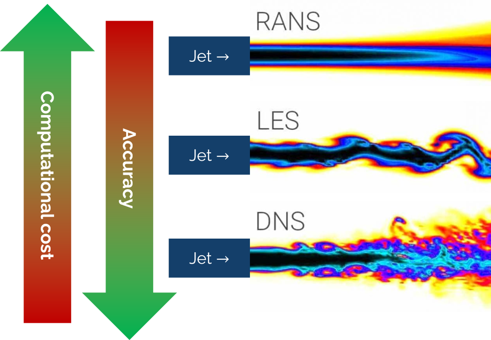
RANS provides us with a time-averaged representation of the flow (we will see later where this time-averaged representation is coming from). LES models some of the smaller scales, but not all, but we can see some instantaneous velocity that deviates from the time-averaged representation. DNS resolves all turbulence, and we can see smaller scales being present compared to LES, although the bulk of the flow is the same. If we were to take the time-average of the flow for both LES and DNS, it would look fairly similar to the RANS representation!

We can also see that as we move from RANS to LES, and from LES to DNS, the resolution (and thus accuracy) increases, but that comes at the cost of increased computational cost. Our job as CFD engineers is to select the best turbulence modelling approach that still captures the bulk flow, while not using more resources than absolutely required.

If we wanted to quantify this computational cost, then we could find scaling behaviour for each turbulence modelling strategy in terms of the Reynolds number. These are given below:

• DNS: Re^3
• LES: Re^2 - Re^{2.5}
• RANS: Re^1

This means that we can roughly say that RANS simulation scales linearly with our Reynolds number, while LES scales quadratically, and DNS to the power of three. Therefore, for high Reynolds number flows, LES and DNS are still not an option, although we see more and more simulations for industrially relevant geometries and Reynolds numbers being performed with LES, although in an academic and research context.

With this introduction on turbulence modelling out of the way, let us review how Direct Numerical Simulations (DNS) work and what we need to take care of in order to resolve all turbulent eddies.

Direct numerical simulations (DNS)

As the name Direct Numerical Simulations suggests, and we have seen above, we are modelling all turbulence length scales with this approach. This means that the momentum equation we are modelling is simply the instantaneous momentum equation we saw previously, i.e.:

\frac{\partial U}{\partial t}+ U\frac{\partial U}{\partial x}=-\frac{1}{\rho}\frac{\partial P}{\partial x} + \nu\frac{\partial^2 U}{\partial x^2}

The instantaneous components for the velocity U and pressure P do include the mean and fluctuating components, i.e. we have

U=\bar{u} + u'\\[1em]
P=\bar{p} + p'

Therefore, since the fluctuating components are explicitly included in this modelling approach, the Reynolds stresses u'u' are as well. Therefore, it does not make sense to speak of DNS as a modelling approach, as no turbulence is modelled, but rather 100% resolved.

This puts restrictions on our time step and mesh size, which were determined by the Kolmogorov micro scale. We saw them previously and had for the length and time scales:

\eta=\left(\frac{\nu^3}{\varepsilon}\right)^\frac{1}{4}\\[1em]
\tau_\eta=\sqrt{\frac{\nu}{\varepsilon}}

The viscosity is a material parameter, i.e. this is set by the fluid (and it may vary based on temperature within the flow domain). The dissipation rate \varepsilon is slightly more difficult to obtain. In our introductory example, we approximated the dissipation rate with mean quantities, but we can also explicitly resolve and calculate it. The equation for the exact dissipation rate is given as:

\varepsilon=\sum_{i=1}^3\sum_{j=1}^3 \nu \overline{\frac{\partial u'_j}{\partial x_i}\frac{\partial u'_j}{\partial x_i}}

This term is typically without the summation symbols, and the so-called Einstein summation convention is used. This notation implies that if an index appears twice (in this case, we have indices i and j), then it is implied that we are summing over all of their component. In this case, both i and j go from 1 to 3, as we have three coordinate directions in a three-dimensional flow. Using Einstein summation convention, we can write the dissipation rate definition in its more conventional form:

\varepsilon=\nu \overline{\frac{\partial u'_j}{\partial x_i}\frac{\partial u'_j}{\partial x_i}}

If we apply the summation now, then we get the following definition:

\varepsilon=\nu\left(
\overline{\frac{\partial u'_1}{\partial x_1}\frac{\partial u'_1}{\partial x_1}} + \overline{\frac{\partial u'_2}{\partial x_1}\frac{\partial u'_2}{\partial x_1}} + \overline{\frac{\partial u'_3}{\partial x_1}\frac{\partial u'_3}{\partial x_1}} +

\overline{\frac{\partial u'_1}{\partial x_2}\frac{\partial u'_1}{\partial x_2}} + \overline{\frac{\partial u'_2}{\partial x_2}\frac{\partial u'_2}{\partial x_2}} + \overline{\frac{\partial u'_3}{\partial x_2}\frac{\partial u'_3}{\partial x_2}} +

\overline{\frac{\partial u'_1}{\partial x_3}\frac{\partial u'_1}{\partial x_3}} + \overline{\frac{\partial u'_2}{\partial x_3}\frac{\partial u'_2}{\partial x_3}} + \overline{\frac{\partial u'_3}{\partial x_3}\frac{\partial u'_3}{\partial x_3}} 

\right)

\\[1em]

\varepsilon=\nu\left(
\overline{\frac{\partial u'}{\partial x}\frac{\partial u'}{\partial x}} + \overline{\frac{\partial v'}{\partial x}\frac{\partial v'}{\partial x}} + \overline{\frac{\partial w'}{\partial x}\frac{\partial w'}{\partial x}} +

\overline{\frac{\partial u'}{\partial y}\frac{\partial u'}{\partial y}} + \overline{\frac{\partial v'}{\partial y}\frac{\partial v'}{\partial y}} + \overline{\frac{\partial w'}{\partial y}\frac{\partial w'}{\partial y}} +

\overline{\frac{\partial u'}{\partial z}\frac{\partial u'}{\partial z}} + \overline{\frac{\partial v'}{\partial z}\frac{\partial v'}{\partial z}} + \overline{\frac{\partial w'}{\partial z}\frac{\partial w'}{\partial z}}

\right)

Here, u', v', and w' are the fluctuating velocity components in the x, y, and z direction, respectively. We haven’t seen these velocity components yet, so let us introduce them for clarity.

In our discussion on where turbulence is coming from in a mathematical sense, we derived the mean flow equations, which showed us that turbulence is generated by the non-linear term. Inserting the Reynolds decomposition for the non-linear velocity term resulted in additional Reynolds stresses. The equation we obtained was given, in one dimension, as:

\frac{\partial \bar{u}}{\partial t}+ \frac{\partial \bar{u}\bar{u}}{\partial x}=-\frac{1}{\rho}\frac{\partial \bar{p}}{\partial x} + \nu\frac{\partial^2 \bar{u}}{\partial x^2} - \frac{\partial \overline{u'u'}}{\partial x}

Well, in the equation that we saw before, the additional Reynolds stresses were written on the left-hand side of the equation. In the equation above, I have written them on the right-hand side, as is commonly done, to indicate that turbulence works against the mean flow (it is taking energy away from it), which is indicated by the minus sign now. We can also multiply the equation by the density (noting that the dynamic viscosity is defined as \mu=\rho\nu) to arrive at:

\rho\frac{\partial \bar{u}}{\partial t}+ \rho\frac{\partial \bar{u}\bar{u}}{\partial x}=-\frac{\partial \bar{p}}{\partial x} + \mu\frac{\partial^2 \bar{u}}{\partial x^2} - \rho\frac{\partial \overline{u'u'}}{\partial x}

This is the form you will commonly see in the literature, where the Reynolds stresses are now given as \rho\overline{u'u'}. As alluded to above, this is a one-dimensional equation, but if we were to write this for a three-dimensional case, we would now gain additional non-linear terms in the y and z directions, containing velocity fluctuations in the y and z directions as well. For each additional non-linear term, we have to add one additional Reynolds stress term, and thus our three-dimensional, mean flow momentum equations can be written as:

\rho\frac{\partial \bar{u}}{\partial t}+ 
\rho\frac{\partial \bar{u}\bar{u}}{\partial x} +
\rho\frac{\partial \bar{v}\bar{u}}{\partial y} +
\rho\frac{\partial \bar{w}\bar{u}}{\partial z}
=-\frac{\partial \bar{p}}{\partial x} +
\mu\frac{\partial^2 \bar{u}}{\partial x^2} +
\mu\frac{\partial^2 \bar{u}}{\partial y^2} +
\mu\frac{\partial^2 \bar{u}}{\partial z^2} -
\rho\frac{\partial \overline{u'u'}}{\partial x} -
\rho\frac{\partial \overline{v'u'}}{\partial y} -
\rho\frac{\partial \overline{w'u'}}{\partial z} \\[1em]

\rho\frac{\partial \bar{v}}{\partial t}+ 
\rho\frac{\partial \bar{u}\bar{v}}{\partial x} +
\rho\frac{\partial \bar{v}\bar{v}}{\partial y} +
\rho\frac{\partial \bar{w}\bar{v}}{\partial z}
=-\frac{\partial \bar{p}}{\partial y} + 
\mu\frac{\partial^2 \bar{v}}{\partial x^2} +
\mu\frac{\partial^2 \bar{v}}{\partial y^2} +
\mu\frac{\partial^2 \bar{v}}{\partial z^2} -
\rho\frac{\partial \overline{u'v'}}{\partial x} -
\rho\frac{\partial \overline{v'v'}}{\partial y} -
\rho\frac{\partial \overline{w'v'}}{\partial z}\\[1em]

\rho\frac{\partial \bar{w}}{\partial t}+ 
\rho\frac{\partial \bar{u}\bar{w}}{\partial x} +
\rho\frac{\partial \bar{v}\bar{w}}{\partial y} +
\rho\frac{\partial \bar{w}\bar{w}}{\partial z}
=-\frac{\partial \bar{p}}{\partial z} + 
\mu\frac{\partial^2 \bar{w}}{\partial x^2} +
\mu\frac{\partial^2 \bar{w}}{\partial y^2} +
\mu\frac{\partial^2 \bar{w}}{\partial z^2} -
\rho\frac{\partial \overline{u'w'}}{\partial x} -
\rho\frac{\partial \overline{v'w'}}{\partial y} -
\rho\frac{\partial \overline{w'w'}}{\partial z}

If we wanted to write this equation again in compact form, we could do so by using Einstein’s summation convention. In this case, we would end up with:

\rho\frac{\partial \bar{u_j}}{\partial t}+ 
\rho\frac{\partial \bar{u_i}\bar{u_j}}{\partial x_i}
=-\frac{\partial \bar{p}}{\partial x_j} +
\mu\frac{\partial^2 \bar{u_j}}{\partial x^2_i} -
\rho\frac{\partial \overline{u'_i u'_j}}{\partial x_j}

Now we can identify the Reynolds stresses as \rho\overline{u'_i u'_j} and we can write them out explicitly as:

\tau=\rho\begin{bmatrix}
\overline{u'u'} & \overline{u'v'} & \overline{u'w'}\\[1em]
\overline{v'u'} & \overline{v'v'} & \overline{v'w'} \\[1em]
\overline{w'u'} & \overline{w'v'} & \overline{w'w'}
\end{bmatrix}

The following symmetry condition holds true for the Reynolds stresses: \overline{u'_i u'_j} = \overline{u'_j u'_i}. For example, we have \overline{u'v'}=\overline{v'u'}. Therefore, we can also write the Reynolds stress tensor as:

\tau=\rho\begin{bmatrix}
\overline{u'u'} & \overline{u'v'} & \overline{u'w'}\\[1em]
\overline{u'v'} & \overline{v'v'} & \overline{v'w'} \\[1em]
\overline{u'w'} & \overline{v'w'} & \overline{w'w'}
\end{bmatrix}

Now we can see that only the upper triangle is unique, i.e. the lower triangle uses components from the upper triangle. Therefore, we only have 6 independent Reynolds stresses, and, since the above construct is a tensor, we also call the Reynolds stresses the Reynolds stress tensor when we talk collectively about all Reynolds stresses.

Returning to the definition of the dissipation rate, we had:

\varepsilon=\nu\left(
\overline{\frac{\partial u'}{\partial x}\frac{\partial u'}{\partial x}} + \overline{\frac{\partial v'}{\partial x}\frac{\partial v'}{\partial x}} + \overline{\frac{\partial w'}{\partial x}\frac{\partial w'}{\partial x}} +

\overline{\frac{\partial u'}{\partial y}\frac{\partial u'}{\partial y}} + \overline{\frac{\partial v'}{\partial y}\frac{\partial v'}{\partial y}} + \overline{\frac{\partial w'}{\partial y}\frac{\partial w'}{\partial y}} +

\overline{\frac{\partial u'}{\partial z}\frac{\partial u'}{\partial z}} + \overline{\frac{\partial v'}{\partial z}\frac{\partial v'}{\partial z}} + \overline{\frac{\partial w'}{\partial z}\frac{\partial w'}{\partial z}}

\right)

We see here that we simply take the derivative of the time-averaged Reynolds stresses, and so the dissipation rate is closely related to the Reynolds stresses themselves. Once we know the dissipation rate, we can compute our Kolmogorov length and time scales as:

\eta=\left(\frac{\nu^3}{\varepsilon}\right)^\frac{1}{4}\\[1em]
\tau_\eta=\sqrt{\frac{\nu}{\varepsilon}}

In our simulation, we have to ensure that our grid size is locally equal to or smaller than \eta, and that our time step is smaller than \tau_\eta. The time step is typically easy to achieve, as we also have the CFL condition to satisfy, which typically requires much smaller time steps.

The length scale, on the other hand, is very restrictive, and this leads to very fine meshes. Since the mesh will be three-dimensional, we are dealing with cells that are potentially arbitrarily shaped elements (though we prefer hexa elements opposed to general polyhedra as these have better diffusive properties), and it may not be clear what the length of a cell is. Therefore, we calculate a characteristic length for each element, which we do by taking the cube root of the element’s volume. This is defined as:

l=\sqrt[3]{V}

Now that we have a characteristic length for each cell, we can compare that against the Kolmogorov length scale \eta. For each cell in the domain, we compute the following resolution operator \Delta:

\Delta =\frac{\eta}{l}

In order to ensure that we are always resolving all turbulence, we aim for a value of \Delta \ge 1 in each cell. If this is the case, our mesh is resolving all turbulence. However, due to the numerical cost of DNS, it is not uncommon to relax this definition to \Delta \ge 0.5, which allows our characteristic length to be twice as big as the local Kolmogorov length scale. This reduces the mesh size requirements substantially while still resolving turbulence to an acceptable level.

We can now calculate this resolution operator \Delta for each cell and visualise with a post-processor. We can then visually identify regions where the mesh needs refinement in order to satisfy either \Delta \ge 1 or \Delta \ge 0.5.

A post-processor like Tecplot or ParaView allows you to calculate how many cells satisfy this criterion, and then you can sum up the volume of all elements that do satisfy this criterion. If you divide this number by the overall volume of the computational domain, then you know how much of your simulation is resolving turbulence well. There may always be elements that locally violate your criterion, and there is not much you can do about it. But if the majority of your domain satisfies this resolution criterion, then you know that you have a high-quality DNS.

This approach assumes that we have already performed a DNS, i.e. we have all Reynolds stresses available. But what if we do not know them beforehand? Typically, we want to design the grid before we run our DNS, so some knowledge of the grid size beforehand would be required.

There are two approaches you can take. The first one is to look at the published literature. Chances are, you are simulating something simple in terms of geometry that was already investigated before. You can then take inspiration from the paper’s mesh settings and use them in your simulation.

The second approach requires you to perform a cheap and simple turbulence simulation, for example, using RANS (discussed in one of the next articles). For example, if you use the k-\varepsilon model, you get an estimate for the dissipation rate for each cell, and so you can use that estimate to compute how well your current mesh would resolve the Kolmogorov length scale. As this is only a modelled dissipation rate, your actual Kolmogorov length scale will be different, but it will give you a usable way to construct your initial mesh.

If your simulation contains any solid walls, you must aim for a y^+ value of at least 1, if not lower, since we want to resolve the entire velocity profile within the turbulent boundary layer.

And this is all there is to DNS. We do not model any turbulence, but instead, resolve all of it. Therefore, the modelling is very straightforward (in that we do not have to model the Reynolds stresses in any way; they are explicitly calculated), but the computational cost is high as a result. By estimating the Kolmogorov length scale before we start our simulation, we can ensure that our mesh will resolve all turbulence to a satisfactory degree.

Summary

This article reviewed how turbulence is generated, both in a physical and in a mathematical sense. We saw the importance of the energy cascade as introduced by Kolmogorov, and how this leads to Kolmogorov’s length, time, and velocity scales that we need to resolve if we want to capture all turbulence. We saw that if we achieve that, then we have performed a Direct Numerical Simulation (DNS), where all turbulence is resolved and none is modelled.

DNS is the simplest form of turbulence modelling, in that we do not have to change or modify the governing equations in any way. They will resolve all turbulent stresses for us. But, this comes at a cost, and DNSs are so computationally expensive that they remain elusive even in academic research for anything more complex than a channel flow application.

Clearly, we need to introduce some modelling into our flow, to make more complex cases computable, and this will be the focus of the next two articles, looking at Large Eddy Simulations (LES) and Reynolds-averaged Navier-Stokes (RANS) simulations.

---

Tom-Robin Teschner is a senior lecturer in computational fluid dynamics and course director for the MSc in computational fluid dynamics and the MSc in aerospace computational engineering at Cranfield University.