Mesh generation in CFD: All you need to know in one article
Do you know the difference between the average CFD user and a world-class CFD practitioner? In most cases, it is the ability to generate a grid for complex geometries, which remains a challenge to this day with the tools we have available. Our desire to simulate ever more complex cases has grown faster than the tools to support this desire. As a result, mesh generation is complicated and a topic we really ought to give attention to, but rarely do.
For every paper that is published on the topic of mesh generation in CFD, there are 42 papers published in the area of turbulence modelling in CFD. This shows how little we care about a topic that is so fundamentally important and typically drives most of the issues we face in CFD. NASA even named it one of their key challenges in their 2030 CFD vision study, yet we treat mesh generation like our drunk uncle at Christmas: you are family, we have to put up with you, but we don't really want to.
In this article, I go through everything there is to know about mesh generation. I spend a lot of time talking about grid quality in this article, not just how it is defined, but also how each quality metric we look at will influence the simulation. In this way, you know exactly what will happen when you have poorly skewed cells or low orthogonality, and then you can decide if this is a problem or not.
We will also look at how structured and unstructured grids are generated, and how the algorithms we use today aim to maximise the grid quality. If you want to take a step towards CFD mastery, then this article will tell you everything you need to know in a single article about a topic you have likely not given a lot of consideration. It is on the lengthier side, but I promise, you will view mesh generation with different eyes after reading this article.
In this series
[custom_category_posts_list category_slug="10-key-concepts-everyone-must-understand-in-cfd"]In this article
- In this series
- In this article
- Introduction
- Mesh elements and their quality - why does it matter?
- Mesh generation
- Summary
Introduction
Mesh generation is one of those topics that splits the masses. Either you love it or hate it, and in all statistical likelihood, you hate it. And, if you don't hate meshing right now, it is very likely you will in the future. Personally, I really like meshing, and it is an almost zen-like activity for me, which I could do for hours. So, I have an uphill battle to fight to make you see the beauty of mesh generation.
I may not be able to convince you today that mesh generation is really not that bad, but if I can take at least some of the frustrations, I'd consider that already a win. In my experience, most of the frustrations come from mesh sensitivities. If you change the mesh slightly, you get disproportionally large changes in your solution, which can be the difference between convergence and divergence.
Contrast that with changes in the numerical scheme, or turbulence model, or linear system of equation solver; these may affect the overall accuracy or global convergence rate, but probably not much more. Thus, you have to spend a lot of time and energy on getting a grid that will allow you to get a result in the first place, and when you are just starting out, your simulations may be diverging rather than converging.
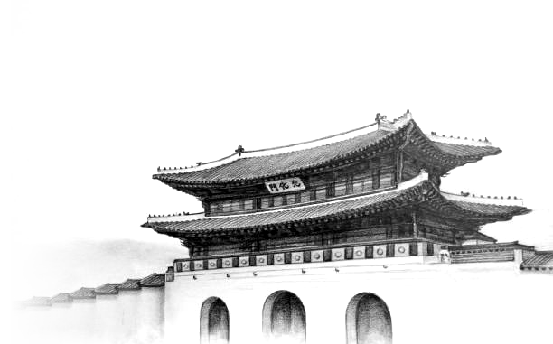
The problem with grid generation can be summarised in the following schematic, which I have dubbed the three pillars of mesh generation:
Here you have the three core elements that underpin any mesh that you create. These are:
- Topology: The topology defines the complexity of your model that you are trying to mesh. Think square box or circular cylinder for a simple topology, and an entire Formula 1 car / IndyCar / Aircraft / etc. for a complex topology.
- Mesh quality: The mesh quality is responsible for a number of things and typically influences the convergence rate, global solution accuracy, and, in the worst case, it can be the difference between convergence and divergence.
- Time to solution: This metric describes how long you will have to wait until you get a solution.
The problem: We can only independently influence two out of these three properties. The third property will be set for us, and it will always negatively affect our simulation. To make matters worse, we really only have a single choice, because the topology is determined by the geometry we want to investigate.
Let's look at a few examples. Let's say we are investigating a complex geometry (topology). We can now choose: Do we either want to have a quick simulation time, which means we have to accept that our mesh will be of poor quality and thus we may get less accurate results, or do we want to strive for a really high-quality grid, requiring some serious compute power?
We could also look at this from another perspective: Say you are a student and you can only run simulations locally on your laptop. This means your computational resources are limited, and unless you want to leave your laptop on for several days and let it compute some CFD cases, you really want to have a fast time to solution. Now you can pick, do you want to also have good results (high grid quality metric)? If so, you will need to limit yourself to simple cases like the flow past a cylinder or an airfoil.
You see how you can use this schematic to determine the bottleneck in your simulation. You may say, "Well, I work for a tech startup, we received a few million in funding, and I can blow it on cloud computing, so time to solution isn't a concern for me". Well, thank you for putting your ignorance on display for us all to enjoy.
Yes, if you have access to a high-performance computing (HPC) cluster, you may think that you can run simulations as large as you want. Therefore, you will not be limited in the other two metrics, and you can achieve a really high grid quality for a complex geometry, right? Well, perhaps, but keep the following in mind:
- There is a limit in how well simulations scale. Throwing more resources (CPU cores, GPU cards) at a simulation doesn't mean infinite speedup. At some point, more resources will hurt you, and simulation times will increase again.
- Scaling only really works for stationary problems. Once you have an unsteady problem, you can't speed up the time stepping; this will always be sequential, unless you try your hand at parallelisation in time techniques, but these haven't matured yet to a point where they become useful (and they are also not available in general-purpose CFD solvers).
- If you have access to an HPC cluster or cloud computing facility with 10 cores, you will find reasons why you need access to 100 cores. If you get 100 cores, you will find reasons why you need access to 1000 cores. If you get 1000 cores, you will find reasons why you need access to 10000 cores. If you get 10000 cores, you will find reasons why you need access to 100000 cores. Can you spot a pattern?
I will say one thing, though: If you have access to some serious computing power, then mesh generation is really simple. If you can make your elements really small, so that they are at least an order of magnitude smaller than the local feature size on your geometry (e.g. curvature/radius on your geometry), then you stand a good chance of generating a really high-quality mesh for even a complex geometry. But as we have seen above, this means you will need to have access to a good HPC cluster or cloud computing service.
There is just one caveat: The environment. You may have heard about global warming, and you may even live in a country where energy prices have soared in the past years. In short, you can run as many simulations as you want with your private cluster, but we should be aware of the environmental cost of doing so.
Here is a simple calculation I did for one of my simulations: I was simulating the flow past small cylindrical tubes using large-eddy simulations (LES). The simulation took 20 days to run on 128 cores. The energy that was required to power and cool the HPC cluster emitted as much CO2 as me driving in a small compact-sized car for about 2000km (I think that is about 1.618 gallon-miles/square-$, rounded, of course, to the nearest milli-Fahrenheit in imperial units, I think ...).
So, even if we have all the computational resources in the world, we ought to think about using them responsibly. Just because we can doesn't mean we should.
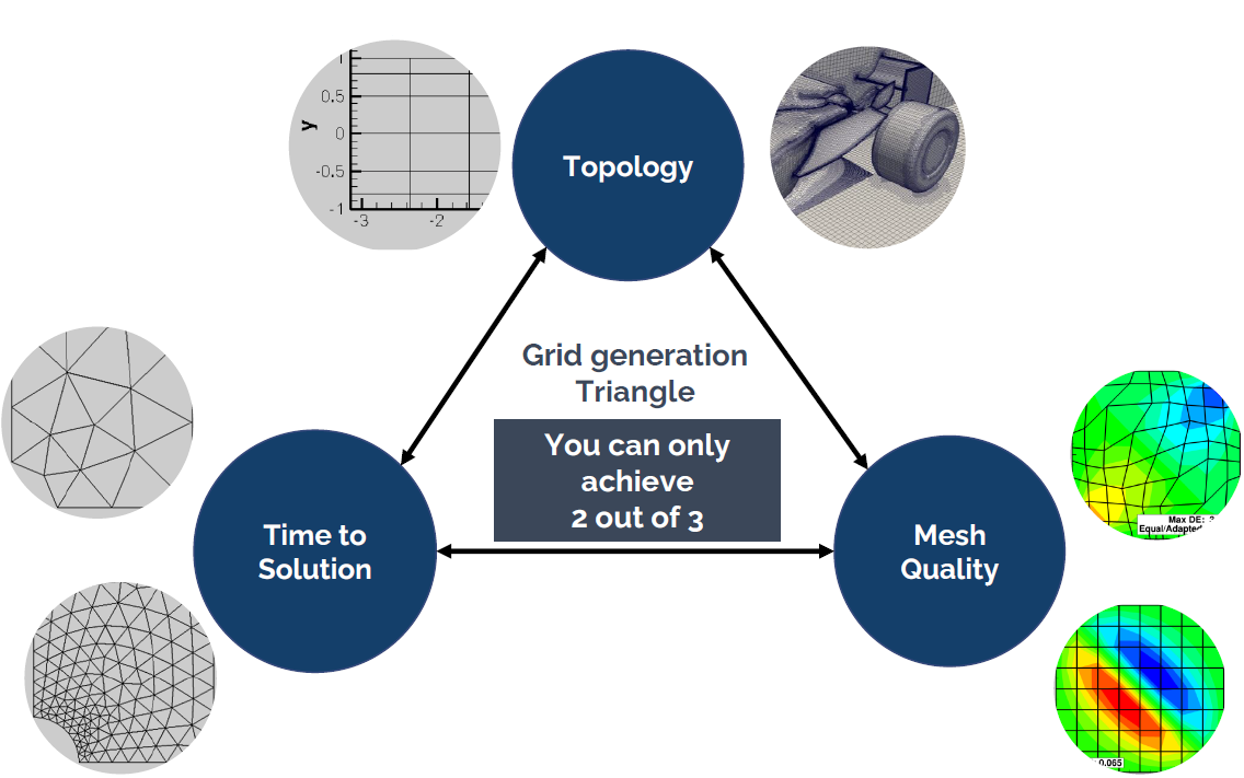
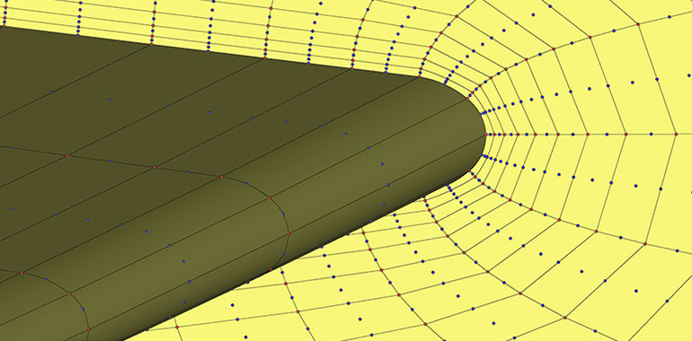
So let's review some common types of mesh generation approaches. The following figure shows the nose section of an aircraft, and a few of the most important mesh generation techniques are used all in a single mesh:
Here, we have the following grid generation techniques at play:
- Body-fitted mesh generation: The red mesh around the aircraft's fuselage is said to be a body-fitted grid, as it follows the geometry of the fuselage and adapts to its curvature.
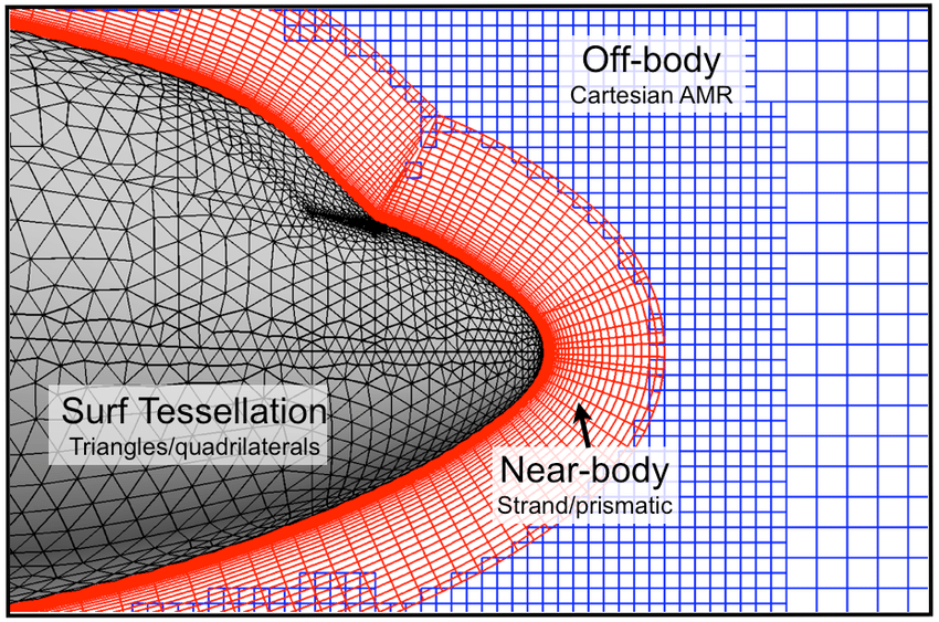
- Conformal / non-conformal mesh generation: A conformal grid is one where the vertices of two adjacent cells overlap. We can see that the blue background mesh has both conformal and non-conformal elements, where some vertices are attached to only one cell. These are also called hanging nodes. The following figure shows the difference between conformal and non-conformal mesh interfaces.
- Overset / Chimera mesh generation: Overset grids, also called Chimera grids, work by having two independent grids intersect each other. They share a common interface across which simulation data is transferred. We see that the body-fitted grid (shown in red) and the background grid (shown in blue) have an overlap, and we use the overset mesh generation approach here to let these two different grids exchange information. Overset grids are powerful for mesh movement, especially if we have complex movement or we don't know the trajectory of the mesh movement.
- Higher-order mesh generation: Typically, when you create a mesh element such as a triangle or quad element, you use linear elements. That is, all edges are composed of two vertices; one at the start, and one at the end. Higher-order mesh generation allows you to have non-linear elements, where edges of a cell may have more than two vertices, allowing for curved edges. This is helpful in resolving large curvatures of complex geometries with very few elements, as seen in the following figure:
Depending on our grid generation needs, as well as the capabilities of our mesh generator, we may adopt any of these techniques when generating our mesh. I should note here, though, that higher-order grids are typically used in conjunction with finite-element methods and thus structural mechanics. They are not yet widespread in CFD. Even if we were to be able to generate a mesh with higher-order elements, our solver also needs to be able to support that, and again, most CFD solvers don't support higher-order elements.
Post-processing is another issue. If you want to visualise higher-order elements, you need to have software that can visualise them for you. As of the time of writing, support for higher-order elements is sparse but some software do support higher-order elements. Suffice it to say, while higher-order elements are the norm for structural simulations, they have yet to become fully adopted in the CFD world.
So, with a basic understanding of meshing techniques and approaches to generate different grids, let us now get into the nitty-gritty details of mesh generation. First up: Mesh quality, and why you really should, nay, must, pay attention.
Mesh elements and their quality - why does it matter?
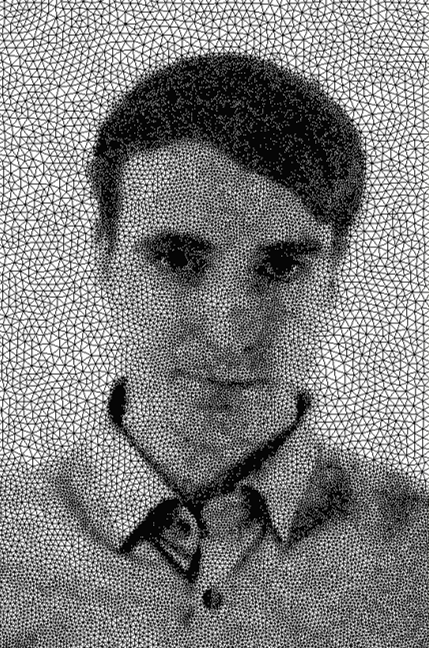
Mesh quality is underrated, underestimated, misunderstood, and frankly, not given the attention it deserves in the literature. Sure, if we want to study homogeneous decaying turbulence in a periodic box, then who cares about grid quality, right? The CFD literature is overly reliant on assuming all we ever want to do is to simulate the simplest of cases, but the real fun only starts once you leave the CFD toy examples behind and dare to mesh a car, an aircraft, or even yourself. This is my attempt:
Look how happy I am! Smiling from cheek to cheek. Well, this is likely the biggest smile you will get out of a German. Don't believe me? Look at the following famous Germans:
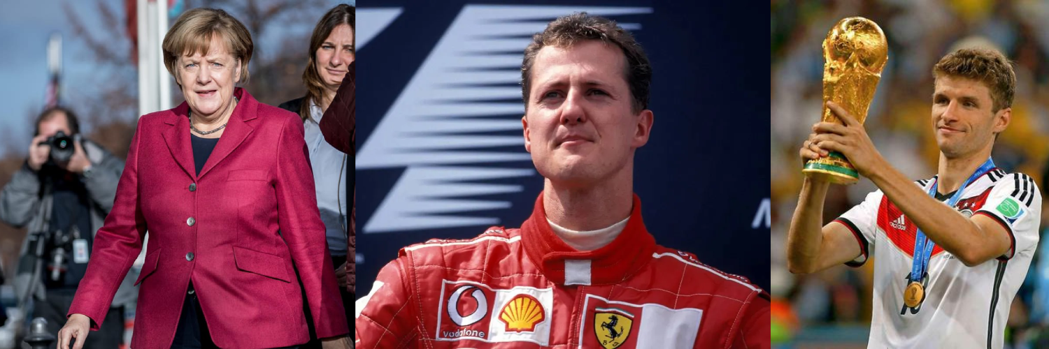
On the left, we have Angela Merkel, the former CEO of Germany after winning an election. In the middle, we have Michael Schumacher after winning another world championship in Formula 1. When he was not busy winning world championships, he always put his well-tempered personality on full display. On the right, you have Thomas Müller after winning a fourth world championship for Germany in 2014 in football. You see, in context, I am smiling quite a lot!
OK, concentrate, Tom, no one cares about your stupid side quests ...
As we have seen in the previous section, unless we are happy to burn the planet to fuel our CFD addiction, a complex geometry typically goes hand-in-hand with some form of poor mesh quality. We can't avoid it. Then, you may check what mesh quality limits your CFD solver recommends. These are not rules written in stone but rather experiential values. You generate your mesh, you may or may not respect these recommendations, your simulation diverges regardless, and you cry a little. This is normal.
To save you from a full-blown, hospitalisation-worthy mental breakdown, let us talk about mesh quality for a bit. After you understand the most important mesh quality metrics (of which there are 4, I would argue), life will become easy again. Well, or at least you will know if you should pre-emptively dial 999 as you start your simulation.
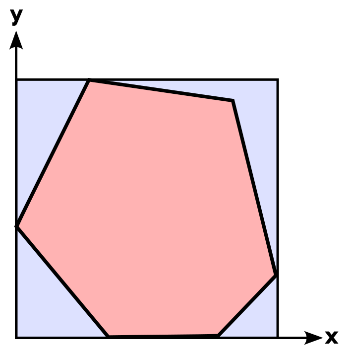
The best way to demonstrate my point is through a case study. We are going to take the most boring case in the world, at least if you have done your PhD in incompressible flows and spent more time with it than your partner (Anyone? Just me?). The case is schematically depicted below:
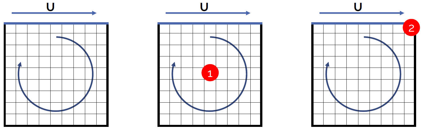
It's a box (yay!), where the left, right, and bottom boundaries are set as solid, stationary walls. The top boundary is also a wall, but it is moving from left to right. In an experiment, we would achieve this by having a box filled with a fluid, where we attach a conveyor belt at the top, simulating the moving wall boundary condition.
In the schematic shown above, I have given you three geometries. The left one is the baseline. This mesh was generated with the best possible mesh quality (we will get onto what that means later). For the case in the middle, I have moved nodes around in the centre of the mesh, so as to reduce the mesh quality in this region. I have done the same for the mesh shown on the right, with the only difference that I have manipulated the mesh in the top right corner.
So, we have the control (baseline), and two grids with reduced mesh quality in two different locations. The question now becomes, what happens to our simulation? Well, the following 5 scenarios are possible:
- Nothing happens; the simulation will be unaffected
- The simulation will diverge
- The convergence rate will be reduced
- The accuracy will be reduced
- The convergence rate and accuracy will be reduced
Make your choice. Ready? Let's move on then. After my overly dramatic introduction to mesh quality metrics, and how they are underrated and getting you hospitalised, we can probably guess that the first option is out. But what about the other 4? Well, let's have a look.
The following overview shows contour plots of the velocity magnitude for the control (baseline), as well as the two other grids. I have generated two grids at each location (location 1 in the centre of the domain and location 2 at the top right corner). I have generated these grids so that we have a case where we have low quality, which is still acceptable, and poor quality, which may affect your simulations negatively.
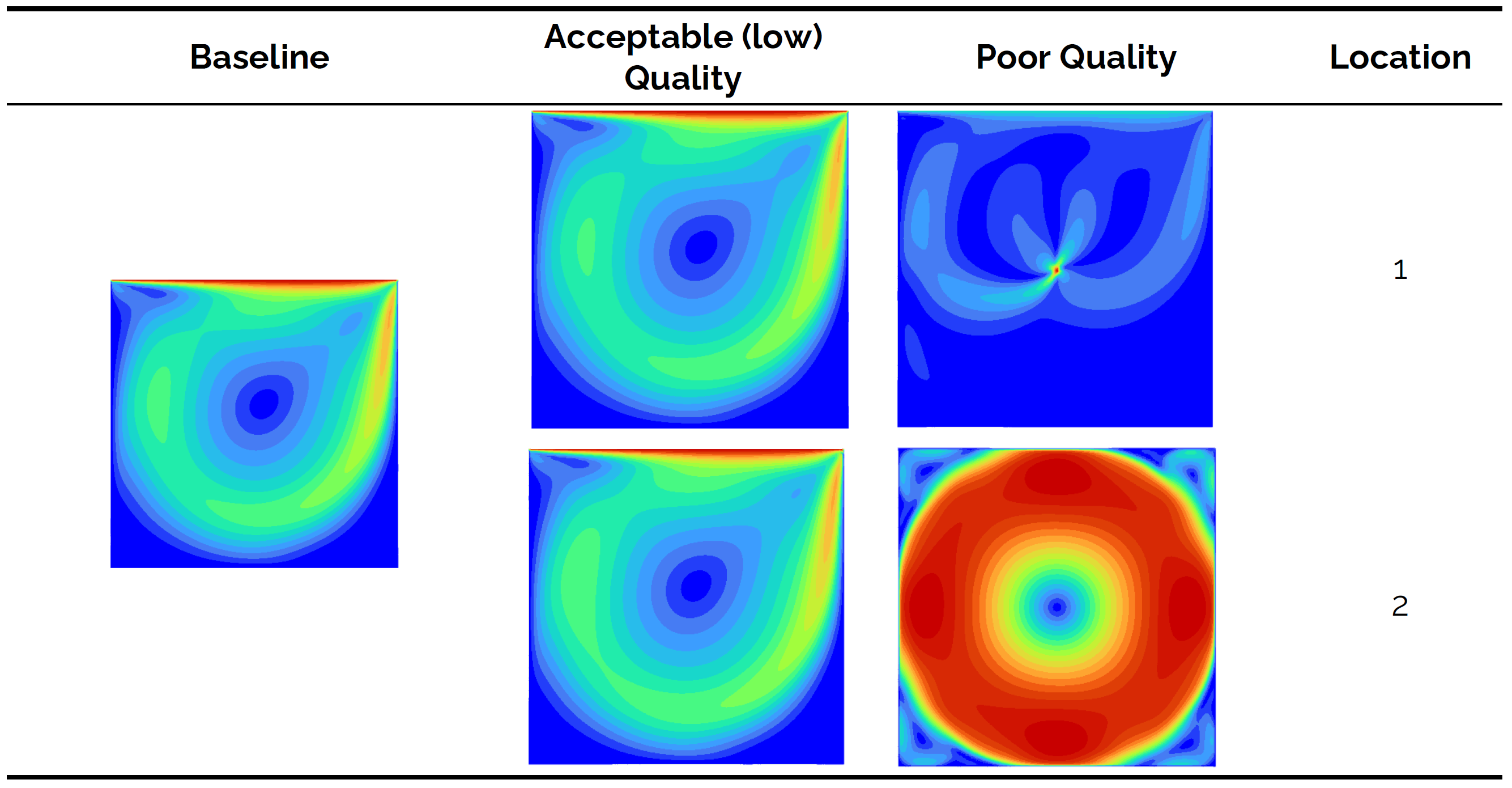
We see from the baseline that a vortex is formed in the centre of the domain. The Reynolds number isn't particularly high (it is 100 based on the length of the top boundary), so for all intents and purposes, this is a laminar flow. Let's look at the result for the low, but still acceptable, quality cases. Both locations 1 and 2 show that the results are slightly different to the control (if we inspect contour lines), but overall we can say that we still have obtained good results.
Looking at the poor quality case, however, we see that we get nonsensical results. For both locations 1 and 2, we get results that do not match the baseline, and for location 1, we can see that we get a singularity of some form that is located at the exact point where the poor mesh quality comes from. OK, so there is definitely an influence on the accuracy of the simulation, but what about the convergence rate? This is shown in the next overview:
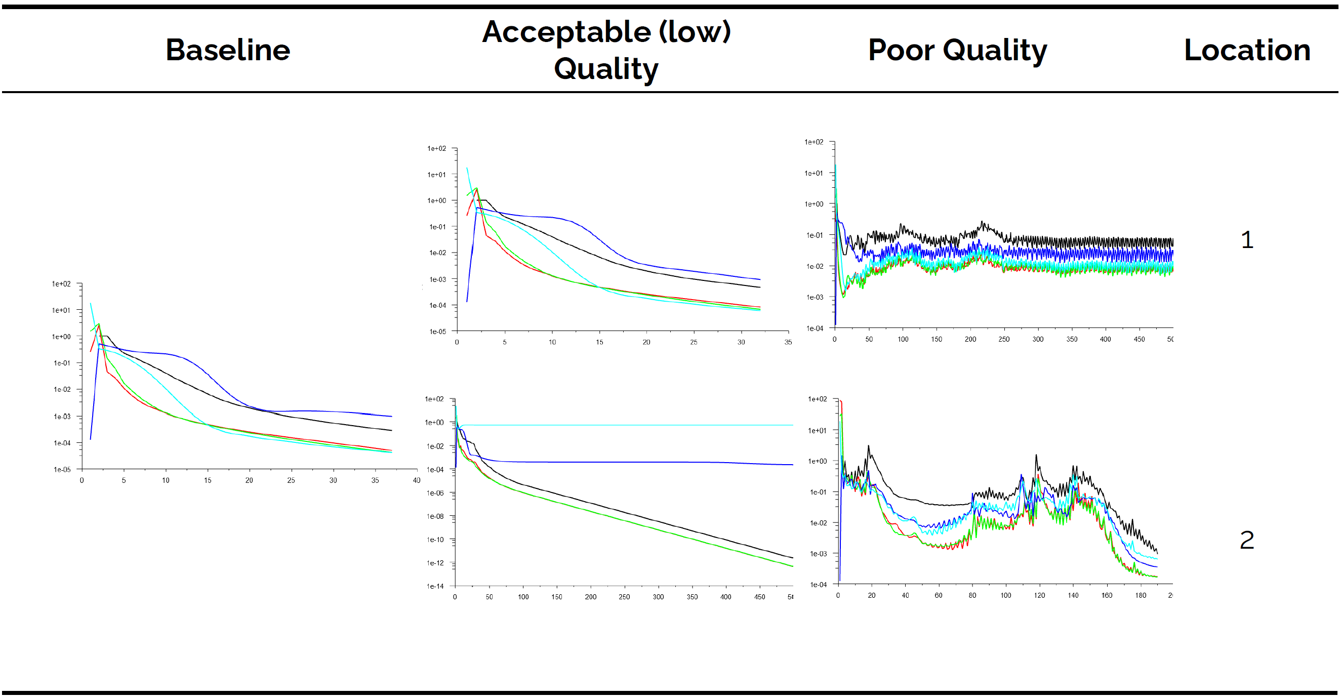
Here, we can see the residuals for the simulation. In general, looking at the residuals to judge convergence is rarely a good idea, but for simple cases without turbulence, you can typically get away with it. The baseline shows convergence after about 37 iterations. The exact value isn't important; we are interested in the trend.
Let's look at the low, but acceptable, quality case. For location 1, the flow is converging; no problem at all here. But at location 2, we see that the residuals for two variables have flatlined. Residual-based convergence checking would not be possible here, and we would typically resort to integral quantity-based convergence checking.
Now, let's turn our attention to the poor quality case. At location 1, there is no convergence. This isn't the biggest problem here. Looking at the residuals, they suggest that we are dealing with a turbulent flow, where residuals typically oscillate in exactly the same manner as we can see here on display. Even worse, at location 2, we get convergence. We know, from the previous contour plots, that we got non-physical results here; even so, we do get convergence in this case.
So what is going on here? Grid quality has the following properties:
- They reduce your convergence rate and may even result in no convergence at all.
- The accuracy may be affected, and you may even converge to non-physical results.
- Even though not shown here, a poor-quality mesh may be responsible for divergence.
To make matters worse, all it takes is just a single cell in which the quality is low. For the case study shown above, I just tampered with the quality of 1 cell. All it took was 1 cell to ruin the entire simulation. So, mesh quality affects the solution globally and not just locally where it occurs. Just like cancer, it spreads from one cell to another until the entire system is affected.
Thus, we have to be vigilant and ensure that we generate a mesh with the best possible mesh quality metrics. So, how do we know if a mesh is good or not? Well, we have mesh quality metrics that tell us exactly how good or bad our mesh is, and we will review them shortly. However, mesh quality is not just a function of the complexity of the geometry we try to simulate but also of the mesh element types we want to use. Let's take a look at them first, and then we will look at the 4 most influential mesh quality metrics.
The group of 10: The fundamental building blocks of any mesh
All you ever need is 10 elements. These are depicted in the following figure:
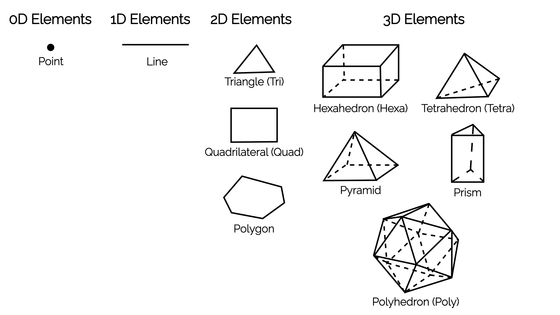
The overview shows elements grouped by their dimensionality. In 0D, we just have a single point, and in 1D, we have a single line. You may ask yourself, what is the point of having a 0D point? Well, if we write an [katex]N[/katex]-dimensional CFD solver, then our boundary conditions will be [katex]N-1[/katex]. So, for a 1D CFD solver, we would be using lines in the domain and [katex]N-1=1-1=0[/katex], i.e. 0D points on the boundaries.
Of more interest are the elements in 2D and 3D. The standard elements we have come to accept for 2D are the triangle and quad elements, while in 3D, we have tetra, hexa, prism, and pyramid elements. In 2D and 3D combined, we have 6 standard elements. However, we also have polygons in 2D and polyhedra in 3D. Polygons can represent any shape in 2D (including triangles and quads), and polyhedra can represent any shape in 3D (including tetra, hexa, prism, and pyramid elements).
So, you could say, all you ever need are just 4 elements: a point, a line, a polygon, and a polyhedron. I would agree with that (and, in fact, I would write my CFD solver in exactly this way, as I just have to implement a single element type and be able to work with any mesh element type), but, for legacy reasons, we like to keep the other 6 standard elements around. Some mesh generators can't generate polyhedra, some mesh formats can't represent them, and so we keep our inferior standard elements around.
They do serve a good educational purpose, though. If I told you that pyramids are a nightmare to deal with, then you may ask yourself, why do we use them in the first place? Well, there is a very specific use case for which we use them, even though we may prefer to avoid them. Can you spot it?
If I told you that a quad-dominant surface mesh is better than a triangle-dominant surface mesh, and that tetrahedra have the ability to fill out any 3D space without any issue, while hexahedra struggle, can you see why Pyramids are good? Both the pyramid and prism elements possess a property that the other elements don't have: they are composed of both quad and triangle surfaces.
If I have a quad-dominant surface mesh and I want to connect that to my tetra-dominant volume mesh, then I need to connect my quads from the surface mesh with triangles from my tetrahedra. Thus, I need a connecting element that has both triangle and quad surfaces. This is why I need pyramids. Prism elements serve exactly the same purpose, only that they connect a triangle surface mesh with tetrahedra in the far field, while allowing for nicely stacked layers between the surface and far field mesh.
These layers, often referred to as inflation layers, are important, as we will see later, to resolve the turbulent boundary layer.
OK, at this point, we need to talk about mesh quality metrics to get the full picture. We will then see how different mesh elements will directly influence the mesh quality, and this will help us appreciate which mesh generation technique may be best suited for the cases we want to simulate.
Mesh quality - your biggest enemy
I have already stressed that it is your mesh quality that will make or break your simulation. If you then decide to be a good CFD practitioner and you want to generate a mesh with high quality, you might look at what mesh quality metrics are available and realise that there are way too many. Yes, if you open any serious mesh generator, you will likely find 20 - 30 different mesh quality metrics. Does it mean we have to check each?
Thankfully, no! Mesh quality metrics are interrelated. You change one, and others will also change. Depending on the mesh quality metrics we look at, it is usually impossible to get a good quality with one metric and then a bad quality with another one. They typically change together, and if you have generated a bad mesh, you won't be able to cherry-pick one or two quality metrics that look good and then claim that your mesh is perfect, despite your simulations diverging.
There are exceptions, and some mesh quality metrics change independently. Regardless, in my opinion, there are only 4 quality metrics you should pay attention to when inspecting your grid. These are:
- Orthogonality or non-orthogonality
- Skewness
- Aspect ratio
- Area or volume ratio
All of these mesh quality metrics will influence your simulation differently, and in the next sections, we will define and establish the influence each mesh quality metric has on your simulation.
Orthogonality/Non-orthogonality
First up, let's talk about the orthogonality property. For this, let us look at the following schematic:
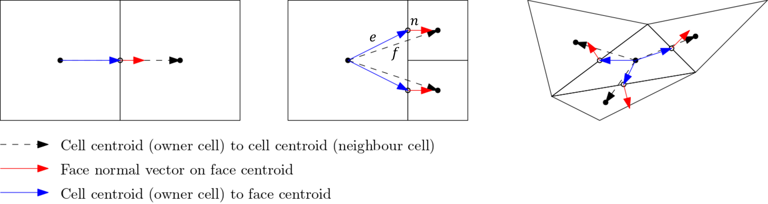
Here, we define three vectors:
- The vector [katex]\mathbf{f}[/katex], shown as a dashed black line, which connects the centroids of two adjacent cells.
- The vector [katex]\mathbf{e}[/katex], shown in blue, which connects a cell centroid with the midpoint of a face.
- The vector [katex]\mathbf{n}[/katex], shown in red, which represents the surface normal vector of the face which connects two adjacent cells.
We use these three vectors to compute the so-called orthogonality property, which is given as:
Q_{Orthogonality}=\min\left(\frac{\mathbf{n}A\cdot \mathbf{f}}{|\mathbf{n}A|\cdot |\mathbf{f}|},\frac{\mathbf{n}A\cdot \mathbf{e}}{|\mathbf{n}A|\cdot |\mathbf{e}|}\right)
\tag{1}
Here, [katex]A[/katex] is the area of the face that connects two adjacent cells. Let's look at what this equation evaluates to. Ignoring the area [katex]A[/katex] for a moment, we see that both numerators in Eq.(1) perform two dot products, or scalar products. We can geometrically interpret the dot product as:
\mathbf{n}\cdot\mathbf{f} = |\mathbf{n}|\,|\mathbf{f}| \cos\theta\tag{2}Here, [katex]\theta[/katex] is the angle between the two vectors. We can solve for the angle [katex]\theta[/katex] and get:
\frac{\mathbf{n}\cdot\mathbf{f}}{|\mathbf{n}|\,|\mathbf{f}|} = \cos\theta\tag{3}Having the magnitude of both vectors in the denominator means that we are now getting a normalised result, i.e. the left-hand side will always evaluate to something between -1 and +1. This is what we would expect for a cosine function. We know that the [katex]\cos(0^\circ)=1[/katex], so if the dot product evaluates to 1, that means that there is no angle between our vectors and they are overlapping.
Looking back at the figure given above, this is the case for the cell arrangement shown on the left. Here, we have all vectors, i.e. [katex]\mathbf{f}[/katex], [katex]\mathbf{e}[/katex], and [katex]\mathbf{n}[/katex] on top of one another. Since there is no angle between these vectors, and we have, as a result, a (normalised) dot product of 1, this means that Eq.(1) must also evaluate to 1, and we have [katex]Q_{orthogonality} = 1[/katex].
However, once we have angles between our vectors and they are no longer aligned with one another, then we get scalar products that are less than one, and as a result, our orthogonality measure will go down. This is shown in the figure above for the cell arrangement in the centre and on the right.
What we can see from this figure as well is that structured grids, consisting of quad (2D) and hexa (3D) elements, will promote high orthogonality out of the box. Sure, curvature in our geometry means that we will get some non-orthogonality, but by itself, quad and hexa elements preserve a high orthogonality. Triangles (2D) and tetra (3D) elements, on the other hand, naturally produce lower orthogonality values, and great effort has to be taken to increase their orthogonality values.
Therefore, we can say that a mesh with perfect orthogonal quality must have a value of 1. A mesh with bad orthogonal quality will approach a value of 0.
Sometimes, you will find people using non-orthogonality instead of orthogonality as a quality metric (yes, I am looking at you, Pointwise, and yes, I know that you changed your name after being bought by Cadence, and I refuse to call you by your full name). This is simply defined as:
Q_{non-orthogonality} = 1 - Q_{orthogonality}\tag{4}In our example above, if we have perfectly aligned vectors, then we have [katex]Q_{orthogonality}=1[/katex] and therefore [katex]Q_{non-orthogonality}=0[/katex].
OK, we know how the orthogonality is defined, so what? Why bother, and why should I care? Excellent question, and to my surprise, no one really describes in the literature what the orthogonality does, and what influence it has on our solution. So let's look at that, but first, we need to quickly discuss numerical integration to make sure we are all on the same page.
Imagine you want to integrate a function but you have no idea what the function is. All you have is several points, which you may have obtained from experimental measurements. What do you do? Well, numerical integration. If you go back to high-school or undergraduate math, you may remember some of the numerical integration techniques, such as the midpoint, trapezoid, or Simpson rule.
Let's take the midpoint rule, and see how we can use that to approximate the area under the function [katex]x=y[/katex] in the interval 0 to 1. Let's say we approximate that with two rectangles/bar elements as shown in the following figure:
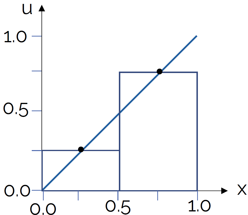
The height of each element is such that the function (or point measurement from an experiment) coincides with the centre of the rectangle/bar element. Then, the idea is to calculate the area of each rectangle/bar element and to sum up these individual areas, which should give us a close prediction of the area under the curve.
The important part here is that we are placing the rectangles/bar elements in such a way that their vertical centerline coincides with the function or point measurements. This means that we will over- and under-predict some area left and right to the function value or point measurement, but these should balance and overall cancel out, as long as the width of our rectangles/bar elements is small enough.
Let's evaluate this integral first analytically, and then numerically. The analytic solution for the integral of [katex]y=x[/katex], or [katex]f(x)=x[/katex] in the interval from 0 to 1 can be obtained as:
\int_0^1 x\mathrm{d}x=\frac{1}{2}x^2\bigg|_0^1=\left(\frac{1}{2}1^2 - \frac{1}{2}0^2\right)=0.5\tag{5}So we would expect the exact area of [katex]y=x[/katex] between 0 and 1 to be 0.5. Just looking at the figure above, we could have probably reasoned that with some intuition without having to evaluate the integral, i.e. we essentially integrate the area under a triangle. If we take another triangle of the same size, and we place it in the upper left part of the plot, then we have two triangles that make a square with an edge length of 1. Therefore, the square must have an area of 1, and so two equally sized triangles must have an area of 0.5.
Ok, let's evaluate the integral numerically. This is done with the following formula:
\int_0^1 x\mathrm{d}x\approx \sum_{i=1}^2 f_i\Delta x = 0.25\cdot 0.5 + 0.75\cdot 0.5 = 0.125 + 0.375 = 0.5\tag{6}Lo and behold, the numerical and analytic evaluation produce exactly the same result. Fantastic! We can throw everything we know about analytic maths out the window and rely entirely on numerical approximations. What's the point of integrals, right? Well, let's look at another example. In the following figure, I have violated the midpoint rule by evaluating the function not at the midpoint of the rectangles/bar elements, but rather some distance to the right. This is shown in the following:
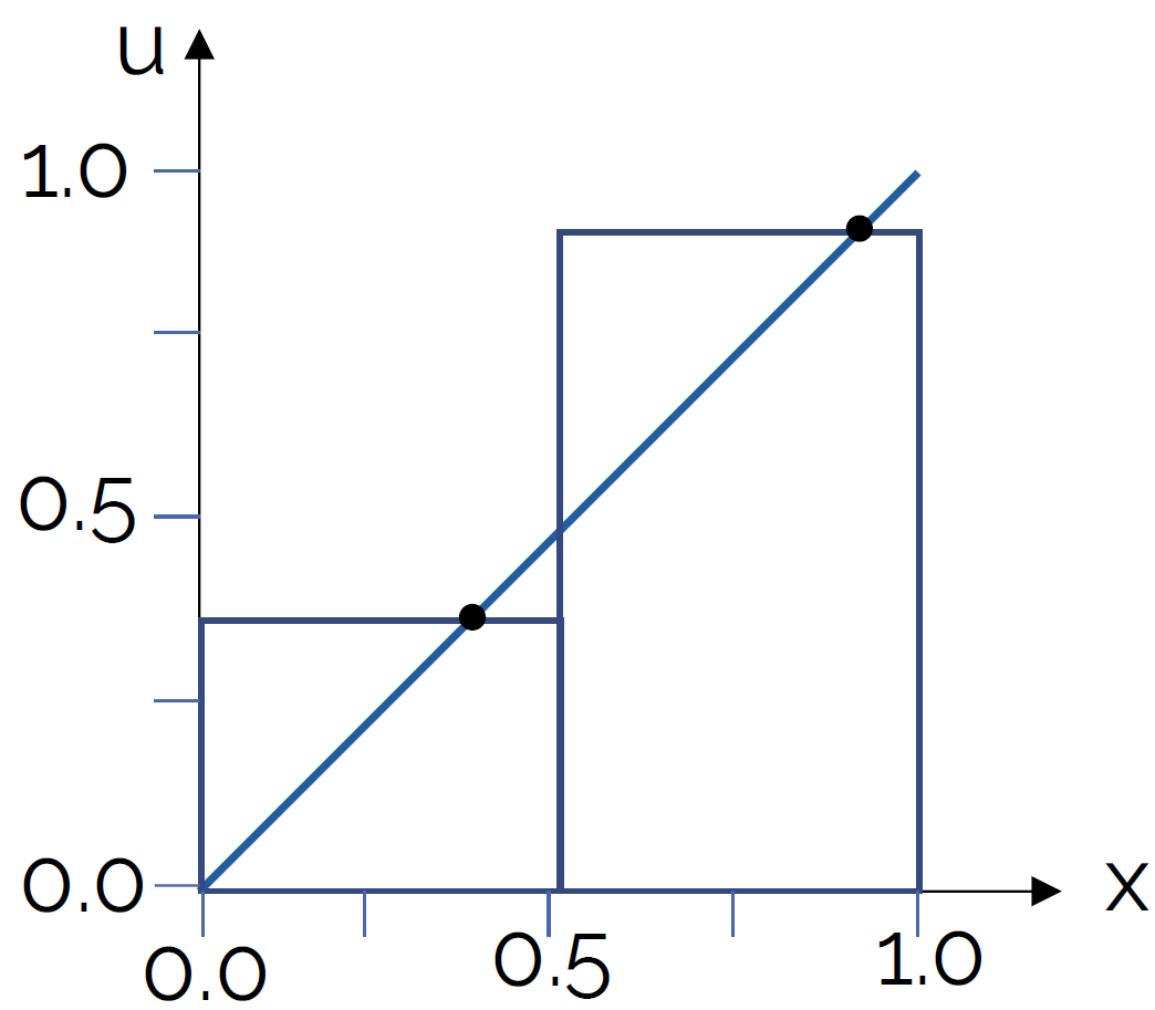
Let's say that the function values, or height of the rectangles/bar elements, now evaluate to 0.4 and 0.9, respectively. Now my numerical integration becomes:
\int_0^1 x\mathrm{d}x\approx \sum_{i=1}^2 f_i\Delta x = 0.4\cdot 0.5 + 0.9\cdot 0.5 = 0.2 + 0.45 = 0.65\tag{7}Hmmm, you might want to open that window and get back all of your analytical math stuff you just threw out of it. Make sure to scoop up all the integrals, you'll need them later ...
So what happened here? We have slightly moved away from the centre of the rectangles/bar elements, and now we have a pretty bad approximation of the area under the curve. This makes sense, as the difference in the area to the left and right of our rectangles/bar elements no longer balances.
But wait, we have only used two elements to numerically evaluate the area, surely we can just throw more than 2 elements at the problem and eventually get the right answer, no? Ok, let's try:
- With a total of 10 elements, we get a value of [katex]\int_0^1 x\mathrm{d}x\approx \sum_{i=1}^{10} f_i\Delta x = 0.53[/katex]
- With a total of 100 elements, we get a value of [katex]\int_0^1 x\mathrm{d}x\approx \sum_{i=1}^{100} f_i\Delta x = 0.503[/katex]
So, well, yes, if we just throw enough resources at our problem, we can get pretty close to the real value, though we will only asymptotically approach the exact value (I'm an engineer by training, I'm ok with asymptotes, if this gives you anxieties, perhaps CFD isn't for you ...).
OK, so how does this all relate to orthogonality or non-orthogonality in our mesh? Well, let's look at the following mesh arrangement:
Imagine we discretise now our governing equations, most likely the Navier-Stokes equations, and we solve them on a mesh that contains the above shown cell arrangements. Given that we have a triangle in there, we have lost the ability to express our mesh as a structured mesh, and so we can only use the finite volume method here (or, finite element method if you feel so inclined) to discretise the equations.
Let's look at the convective term [katex](\mathbf{u}\cdot\nabla )\mathbf{u}[/katex] and discretise it in 1D. We could do it for two or three dimensions as well, but the results will be exactly the same with just more terms, so I am keeping it simple here. Using the finite volume discretisation, we get:
\int_V u\frac{\partial u}{\partial x}\mathrm{d}V = \int_S \mathbf{n}\cdot u \,\mathrm{d}S \approx \sum_{i=0}^{nFaces}\mathbf{n}_i u_i A_i
\tag{8}
First, we take the convective term, i.e. [katex]u(\partial u/\partial x)[/katex] and integrate that over a control volume, which coincides with the volume (area in 2D) of our computational cell (i.e. the two that we see above in the figure). Then, we use the Gauss theorem to transform the volume integral into a surface integral, which we do as surface integrals are conservative while volume integrals aren't. If you want to know why, have a look at Why is the Gauss theorem king?.
Also, if you need a refresher on the finite volume method in general and how to use it to discretise the various terms in the Navier-Stokes equations, I have written an entire section on that, which you can find in my article How to discretise the Navier-Stokes equations.
We approximate the surface integral by summations, where we are now looping over each face (3 for the triangle, 4 for the quad) and then compute the product given after the summation symbol, i.e. [katex]\mathbf{n}_i u_i A_i[/katex]. Here, [katex]\mathbf{n}_i[/katex] is the surface normal vector, pointing in the normal direction of the surface (this is the red vector shown in the figure above). [katex]A_i[/katex] is simply the surface area (or length in 2D). What about [katex]u_i[/katex]?
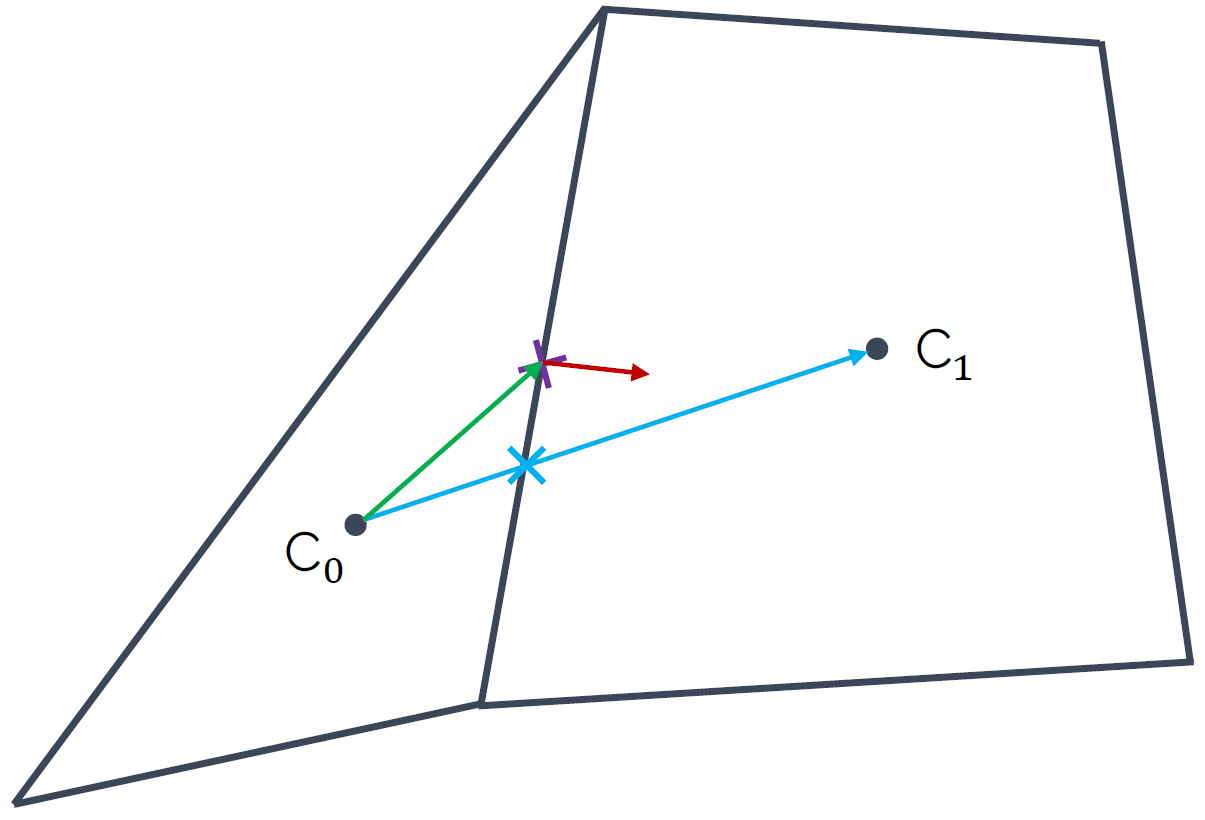
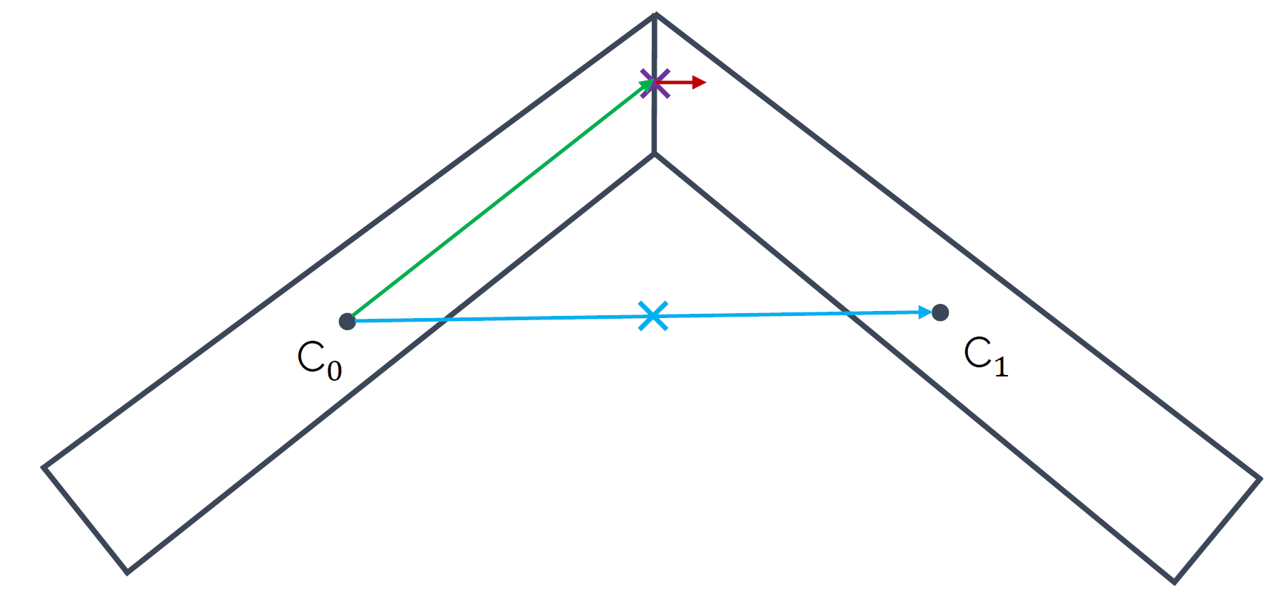
Look at the figure above again. [katex]u_i[/katex] is the velocity component at the face centre, i.e. where the normal vector (shown in red) is located. But we only have the velocity available in each centroid; this is where we store our flow variables like velocity, pressure, temperature, and so on. Thus, we need to interpolate it to have it at the face, which we do by taking a weighted average of the velocity component [katex]u[/katex] from both centroids, i.e.:
u_f = w_1 u_{C_0} + w_2 u_{C_1}\tag{9}The weights are chosen so that the value [katex]u_f[/katex] is obtained on the face. But where is this value of [katex]u_f[/katex], i.e. the velocity component on the face [katex]f[/katex], now available? Look again at the figure above, we get [katex]u_f[/katex] where the blue vector intersects the face. This is marked with the blue cross, and we can see that this is not in the centre.
Bringing this back to our discussion on numerical integration and the inaccuracies we get by evaluating integrals away from the midpoint of the rectangles/bar elements, we see that non-orthogonality in our mesh results in flow variables being evaluated off-centre on cell faces, resulting in inaccurate surface integral approximations.
In other words, the more non-orthogonality we have in our mesh, the more inaccuracy we will get in our results. For this reason alone, despite having developed sophisticates solvers that can work with pretty much any mesh you throw at them, if we had a choice and we lived in an ideal world, people would still use structured grids, even for complex geometries, just because it gives you an edge in terms of accuracy.
We can summarise the effect of non-orthogonality in our mesh with the following schematic plot:
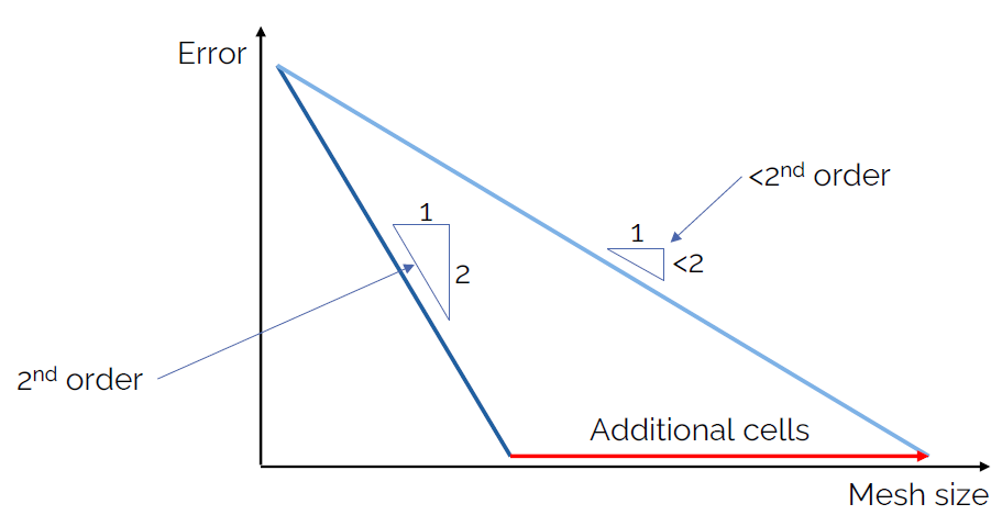
If we assume that we could measure the error (i.e. we have an analytic solution available, which is the case for the simplest of flows), then we can compare our solution to it and compute what the error is. The is what is plotted on the y-axis. On the x-axis, we have the number of cells we use in our mesh.
Looking at the dark blue line first, which is on the left of the plot, we see that for every step we take to the right, we go 2 steps down in our plot. We can say that the slope is 2, and this means that whatever numerical scheme we used to obtain this result is second-order accurate. This is something you can see very well for yourself if you implement various first- and second-order numerical schemes for the advection equation, for which we have an analytic solution available.
Ok, so now, let's introduce some non-orthogonality. We said that this will make our result less accurate, but we also saw that if we just use more integration points (or, more cells in our mesh), then we will be able to eventually reach the same result, at least asymptotically (at least in theory, in practice, we make so many approximations that we won't see this asymptotic behaviour). This is the light blue line in the figure above.
As a consequence, we can see that if we go one unit to the right, we will not be able to go down 2 units, and thus, the order of our scheme has dropped from second-order to whatever value we are obtaining now from this plot. This, non-orthogonality manifests itself by reducing the order of our numerical schemes.
If you carry out a grid dependency study, you will get, among other results, also a measure for the numerical order. Thus, you can directly compute the order that you actually achieved in your simulation. You can get unrealistic values for the order if you don't carry out the grid dependency study correctly, so keep this in mind.
Finally, if we talk about non-orthogonality, you might have read a bit more, and you know about non-orthogonal correction. What is this all about?
We have looked at what happens when we interpolate a velocity field from centroids to the faces, or, let's use a generic variable [katex]\phi[/katex], which could be velocity, pressure, temperature, etc. But, when we deal with diffusive terms in the Navier-Stokes equation, i.e. [katex]\nu\nabla^2\mathbf{u}[/katex], our discretisation looks slightly different. Let's look at its finite volume approximation for a 1D case as well:
\int_V \nu\frac{\partial^2 u}{\partial x^2}\,\mathrm{d}V = \int_S \nu\cdot \mathbf{n}\frac{\partial u}{\partial x}\,\mathrm{d}S \approx \nu \sum_{i=0}^{nFaces} \mathbf{n}_i \frac{\partial u}{\partial x}\bigg|_i A_i\tag{10}Here, we use the Gauss theorem to express a volume integral as a surface integral, losing one derivative. However, since we have a second-order derivative, instead of losing the entire derivative, we only reduce it to a first-order derivative. If this is unclear, we could have also written the expression as:
\int_V \nu\frac{\partial^2 u}{\partial x^2}\,\mathrm{d}V = \int_V \nu\frac{\partial}{\partial x}\frac{\partial u}{\partial x}\,\mathrm{d}V\tag{11}Now, using the Gauss theorem, we loose the first part of the derivative, i.e. [katex]\partial/\partial x[/katex]. Thus, when we approximate the diffusive term, we have to interpolate gradients now to the face, instead of just the scalar or vector quantities as we did for the convective term before. Let's return to the two cells we saw before, here reproduced for simplicity (we all hate scrolling, don't we?):
At the cell centroids [katex]C_0[/katex] and [katex]C_1[/katex], we now need to compute the gradients, i.e. [katex]\partial u/\partial x[/katex], or, more generally, [katex]\nabla \mathbf{u}[/katex], and we need to now interpolate these gradients to the face. Thus, we can use our weighted interpolation we saw before as:
\nabla\mathbf{u}_f = w_1 \nabla\mathbf{u}_{C_0} + w_2 \nabla\mathbf{u}_{C_1}\tag{12}Fluxes at faces are evaluated along the normal direction of that face, i.e. along the red arrow in the figure above. But our gradient is now available along the blue arrow, and both the blue and red arrows, or vectors, are not parallel. Thus, if we were to use this gradient now, we would be making an error in our viscous flux calculation. Therefore, we split our gradient into an orthogonal-like and a non-orthogonal-like contribution:
\nabla\mathbf{u}_f = \underbrace{\nabla\mathbf{u}_f \cos\theta_{\mathbf{n},r_{C0C1}}}_\text{orthogonal-like} + \underbrace{\nabla\mathbf{u}_f \cos (1-\theta_{\mathbf{n},r_{C0C1}})}_\text{non-orthogonal-like}\tag{13}Here, the angle [katex]\theta_{\mathbf{n},r_{C0C1}}[/katex] is the angle between the normal vector at the face (red arrow) and the vector connecting the two centroids [katex]C_0[/katex] and [katex]C_1[/katex] (blue arrow). For orthogonal grids, without any non-orthogonality, we have [katex]\theta_{\mathbf{n},r_{C0C1}}=0[/katex].
Let us now evaluate the gradient directly, i.e. we write it in a discretised form. Then we get:
\nabla\mathbf{u}_f = \underbrace{\frac{u_{C_1} - u_{C_0}}{r_{C0C1}} \cos\theta_{\mathbf{n},r_{C0C1}}}_\text{orthogonal-like} + \underbrace{\frac{u_{C_1} - u_{C_0}}{r_{C0C1}} \cos (1-\theta_{\mathbf{n},r_{C0C1}})}_\text{non-orthogonal-like}\tag{14}Here, [katex]r_{C0C1}[/katex] is again the vector connecting the two centroids. So, with this equation, we have found a way to correct our gradient so that it points now in the direction of the normal vector, so that our viscous force calculation is corrected (by the non-orthogonal correction step). Our inviscid fluxes (i.e. our convective term) are unaffected by this, and we still have inaccuracies (reduction in the order of the numerical scheme) due to non-orthogonality.
So, just because we apply non-orthogonal correction, it doesn't mean we get rid of the underlying problem. A high-quality mesh, with as little non-orthogonality as possible is still what we would desire. There is no free lunch, I suppose ...
Skewness
The second quality metric I want to look at is the skewness. Before we do that, I have to warn you that there are as many different skewness definitions as there are Kim Jong-Un body doubles (yes, why not, I am using the sun as a source here, legit journalism).
The skewness definition I will introduce here is the equiangle skewness. This is the easiest to understand in my view, and you will find it commonly being used in the wild. The good news is that all the different kinds of skewness definitions measure the same thing, but they are just differently defined. So, even if your software uses a different skewness definition, the discussion in this section will still be relevant (but have a look at how it is defined).
The equiangle skewness states that elements that have the same angle in all corners have no skewness. A triangle in which all corners have an angle of [katex]60^\circ[/katex], for example, will have no skewness. A quad element where all angles have a value of [katex]90^\circ[/katex], will also not have any skewness. Thus, equiangle skewness is a measure by how much the largest and smallest angles will deviate from this ideal angle. This is shown in the following figure:
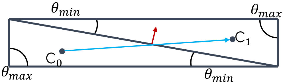
Here we have two triangles where the maximum angle [katex]\theta_{max}[/katex] is [katex]90^\circ[/katex], which is [katex]30^\circ[/katex] more than its ideal angle (the equiangle). The smallest angle [katex]\theta_{min}[/katex] is also well below [katex]60^\circ[/katex] for both triangles. In order to compute the equiangle skewness, we need to determine [katex]\theta_{min}[/katex] and [katex]\theta_{max}[/katex], as well as the equiangle [katex]\theta_e[/katex], i.e. we have [katex]\theta_e=60^\circ[/katex] for a triangle and [katex]\theta_e=90^\circ[/katex] for a quad element. Then, we can compute the equiangle skewness using the following formula:
Q_{skewness}=\max\left(\frac{\theta_{max}-\theta_e}{180^\circ - \theta_e}\, , \,\frac{\theta_e - \theta_{min}}{\theta_e}\right)\tag{15}We can see from this formula that if we have [katex]\theta_e=\theta_{max}=\theta_{min}[/katex], then [katex]Q_{skewness}=0[/katex]. Thus, unlike the orthogonality quality metric, our mesh will have the lowest skewness for a value of 0. As we approach a value of 1, we will start to see skewness-related problems. This is the point where you should check how your skewness is defined in your solver. It might be the same way, it might be the opposit way around.
Skewness and mesh non-orthogonality are very closely linked. In general terms, if you have a low orthogonal quality, your skewness will not be much better. Take a look at the following figure:
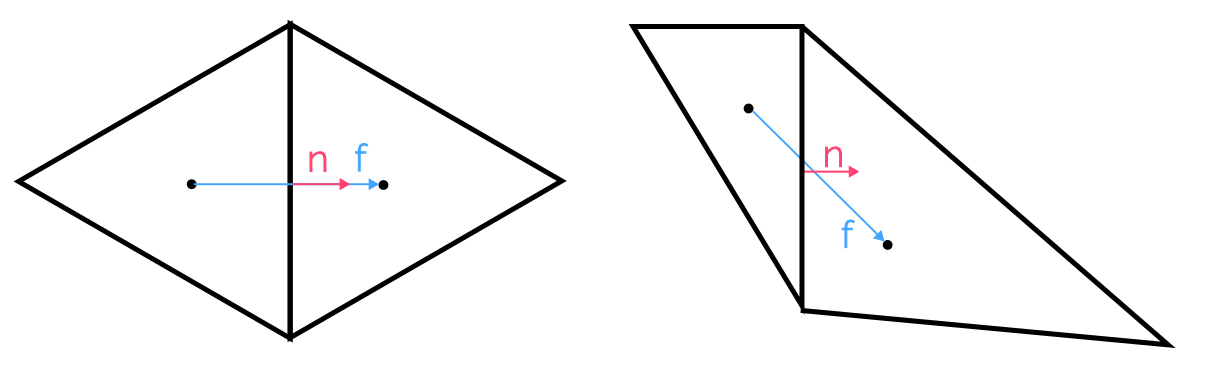
Here, the cell arrangement on the left shows two triangles where each corner has an angle of [katex]\theta=60^\circ[/katex], i.e. both are equilateral triangles and the skewness will be zero as a result, i.e. we have [katex]Q_{skewness}=0[/katex]. The cell arrangement on the right, however, shows two triangles which have different angles in each corner, and, as a result, we get [katex]Q_{skewness} \gt 0[/katex].
At the same time, we can see what the skewness does to our vector [katex]\mathbf{f}[/katex], which connects the two cell centroids, and the normal vector of the face [katex]\mathbf{n}[/katex]. As the skewness increases, we see that these two vectors become more and more misaligned with each other. This will then result in non-orthogonality. Why is this important?
Generally speaking, we can look at either the skewness or the orthogonality and try to improve one of these metrics. If we do, we can expect to proportionally improve the other quality metric as well (I can't think of an example in which this would not be the case; if you can think of an example, send me an email at ElonMuskOffice@TeslaMotors.com and I'll happily engage with you in an in-depth discussion on mesh quality metrics!).
The equiangle skewness is defined for cell properties, i.e. we need to know what the angles are within each element which is easy to conceive for 2D elements, but it may already get more difficult for 3D elements, such as a prism element, where we have both triangles and quad elements (in which case, we may want to use a different skewness definition). If you try to define an equiangle for a polyhedron, you'll soon realise that the equiangle skewness definition only works for simple shapes.
A common workaround is to look at just the angle and use that as a quality measurement. If angles get close to [katex]0^\circ[/katex] or [katex]180^\circ[/katex], then we are in trouble. It is common to say that we do not want to go below [katex]30^\circ[/katex] or above [katex]150^\circ[/katex] if we are looking at just the angle.
Alternatively, we can ignore the skewness and just look at the orthogonality. As we have established, both quality metrics are closely linked, but the orthogonality metric is entirly defined by the properties of the face and centroid properties; the shape or type of the cell is irrelevant. Thus, the orthogonality quality metric can always be defined, even for arbitrary polygons (2D) or polyhedra (3D), and as a result, you will find it used in most solvers as the default quality metric.
As an example, Fluent meshing uses skewness to measure the surface mesh quality (which is always generated with triangles, thus it can be easily computed). But once you generate a volume mesh, the quality metric changes to orthogonality, as we are now dealing with tetrahedra, hexahedra, and polyhedra, i.e. arbitrary mesh elements.
Since skewness and orthogonality are closely linked, all of the issues we get with non-orthogonality are also true for skewness, i.e. our numerical schemes will see a reduction in their order, and we need more cells to get to a similar level of accuracy compared to a grid without any skewness or non-orthogonality.
However, there is a different issue that arises specifically for skewed cells. For this, we need to investigate a somewhat academic example, but it will help us to understand what skewness is doing. For this, we first need to understand what a passive scalar is. A passive scalar is just that, a scalar field which is passive, i.e. it moves together with the bulk flow but it does not influence it (otherwise it would be an active scalar).
A passive scalar field could represent anything, but typically, we think of passive scalars as some form of concentration field. For example, if you run a water channel and you introduce some dye, the dye would follow the main flow, but it would not change it. If you run a wind tunnel test and you introduce particles for PIV measurements, these would be passive scalars as well. Or you use smoke to visualise pathlines, the smoke would also be a passive scalar, as seen in the following video:
Clouds could also be seen as passive scalars, well, they certainly have their own dynamics, but if there is a strong current of air, the clouds will move with the air and deform according to local shear stresses. I think (or hope?!) you get the idea ...
With our new knowledge on passive scalars, let's put that into action. Imagine we want to simulate the flow through a square domain, where we have a constant inflow velocity on the left of the domain. The flow is going through the domain and leaving it on the right side of the square domain. We solve for the passive scalar everywhere in the domain, and we say that we have a concentration of 1 in the upper half of the domain, and a concentration of 0 in the lower half of the domain.
This is shown in the following figure on the left:
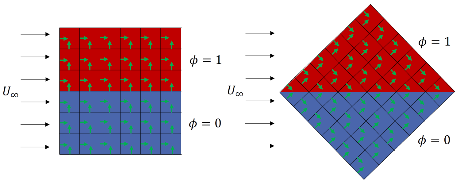
Here, the red region indicates the concentration of the passive scalar of 1 (i.e. 100% concentration, think of this area being filled with smoke) while the blue region indicates no passive scalar concentration (i.e. no smoke can be found here). And now, I rotate the domain by [katex]45^\circ[/katex], though my boundary and initial conditions remain the same, i.e. the flow is still coming from the left, going to the right, and the passive scalar is still initialised the same way, with a horizontal separation between the two phases.
At this point, we need to talk about the mathematics of the passive scalar. The transport equation of a passive scalar is just a generic transport equation, which we have already (ab)used a lot when we looked at creating transport equations for turbulence RANS and LES models. It is given by:
\frac{\partial \phi}{\partial t} + (\mathbf{u}\cdot\nabla)\phi = \Gamma \nabla^2 \phi + S
\tag{16}
Here, the first term is responsible for evolving the passive scalar [katex]\phi[/katex] in time (think of looking at a fixed point in space and see how the passive scalar is changing here), the second term is responsible for its transport (think of it as a particle moving with the mean flow [katex]\mathbf{u}[/katex]), the third term is how it diffuses in space, and the forth term is a source term.
In our case, let's simplify things and set [katex]S=0[/katex], i.e we don't consider any sources. Let's also set [katex]\Gamma=0[/katex], i.e. we don't want to have any diffusion. If we suppress any diffusion, we would expect the passive scalar to simply move from the left to the right, and we would not expect to see any changes at the interface, i.e. where the passive scalar jumps from 0 to 1.
In the following, I have simulated this on three separated domains. The first simulation, shown on the left in the video below, is the case where the domain is not rotated. The diffusion coefficient [katex]\Gamma[/katex] is set to zero. The second simulation, shown in the centre, is the same as the first, except that the diffusion coefficient is set to something greater than zero, i.e. we have [katex]\Gamma \gt 0[/katex].
Finally, the third simulation, shown on the right, shows the simulation with [katex]\Gamma=0[/katex], i.e. no diffusion, but with a [katex]45^\circ[/katex] rotated domain. Also, I have placed a vertical line through the centre of each simulation, and this is shown at the bottom, where the y-axis shows the concentration field and the x-axis the distance along the vertical line.
When the domain is rotated (shown on the right), even though the diffusion is turned off by setting [katex]\Gamma=0[/katex], it shows the same behaviour as the domain that is not rotated but where the diffusion coefficient is set to a non-zero value (shown in the middle), i.e where we have [katex]\Gamma \gt 0[/katex]. What's going on here?
To understand what is happening, I need to give you one additional piece of information, but first, let's look back at the figure above, where I introduced the cases. I have, conveniently, left the face normal vectors in the domain. In the case where the domain was not rotated, all normal vectors were either perfectly aligned with the flow or perfectly normal to it. In the case of the rotated domain, all normal vectors had a [katex]\pm 45^\circ[/katex] angle to the flow direction.
The final piece of information I need to give yoiu is how the variables were interpolated to the faces. I used an upwind-based scheme here. But you may ask yourself, why does this matter?
In any upwind-based scheme, we go to a face and check the direction of the flow. Based on this direction, we determine which is the upwind direction, i.e. the direction against the flow, and then we select properties from the cell that is in the upwind direction, for stability. We looked at upwind and stability of interpolation in my article on numerical schemes, which you may want to go through if you need a refresher.
If we are now on a face which has a [katex]45^\circ[/katex] orientation to the main flow, the upwind direction is somewhat arbitrary. Take a look at the following image:
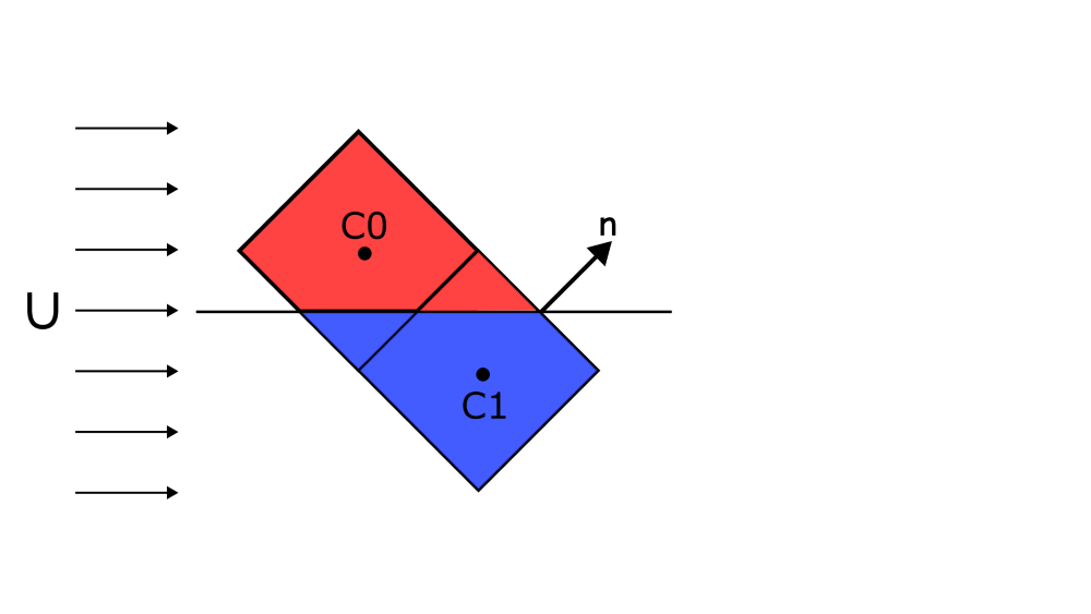
For the normal vector [katex]\mathbf{n}[/katex] as shown in the figure, what is the upwind cell? [katex]C0[/katex] or [katex]C1[/katex]? If we changed the flow direction so that it would have a slight flow component in the positive vertical direction, then the upwind cell would be clearly [katex]C1[/katex], and if we gave the main flow a slight negative vertical component, then the upwind cell would be clearly cell [katex]C0[/katex]. But in this case, and in the simulation we have looked at above, there is no clear upwind cell, and both are equally likely.
Which one does the simulation take? Well, this is a random event over which we have no influence. Sometimes it will be [katex]C0[/katex], and sometimes it will be [katex]C1[/katex]. The problem with this is, as shown in the figure above, at least schematically shown, if [katex]C0[/katex] has a concentration field of [katex]\phi=1[/katex] and [katex]C1[/katex] has a concentration field of [katex]\phi=0[/katex], then this random selection of the upwind direction means that we sometimes get [katex]\phi=1[/katex] and sometimes [katex]\phi=0[/katex] when we use an upwind scheme to get the value ofg [katex]\phi[/katex] at cell faces that are near the interface.
This results in a phenomenon that is called false diffusion, for obvious reasons: If we look at the simulation above again, we can see that despite having turned off the physical diffusion, i.e. by setting [katex]\Gamma=0[/katex], we get numerical (false) diffusion in the case where we have rotated our domain. How does this relate to skewness?
Well, to make one thing clear, the simulation I have performed above has no skewness and no non-orthogonality. But, skewness, in general, has the effect of having misaligned normal face vectors with the mean flow direction, especially if you are considering a triangular, unstructured mesh. So the simulation mimics for us what would happen if we had misalignment due to skewness, even though we do not have any skewness in this case.
Thus, the effect of skewness is non-physical numerical (false) diffusion. The more skewness we have, the more false diffusion we get, resulting in gradients that are smeared/smoothed, which reduces the overall accuracy of our simulation.
Apart from the obvious fact that we probably want to have a highly accurate simulation, let's look at the real danger of skewness. For that, let us look at the flow past a curved surface, where an initially attached boundary layer detaches at a specific point. This is schematically shown in the following image:
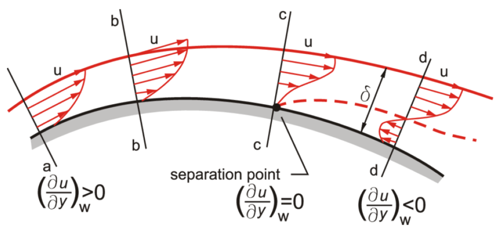
Going from the left to the right, we see that we have a positive velocity gradient, with all the velocity components in the velocity profile pointing from the left to the right, i.e. in flow direction. As the boundary layer develops along the curved surface, it entrains more and more fluid from the undisturbed freestream and grows in size. Due to viscous effects, the growing boundary layer is slowing down, which results in the near-wall pressure rising.
Once the near-wall pressure reaches the same magnitude as the pressure in the freestream, the boundary layer is no longer able to follow the curved surface and detaches from it. This is shown at location c. As we move further downstream, for example, to location d, we can see that the detached boundary layer has developed a recirculation area underneath it, resulting in a negative velocity gradient in the wall-normal direction (now the flow points from the right to the left, against the main flow direction).
We often use the velocity gradient in the wall-normal direction to judge when a flow has separated. We can see from the figure above that this is the case when the velocity gradient is exactly zero in the wall-normal direction and changes its sign, in this case, from positive to negative. But flow separation is not the only time we care about the velocity gradient. Let's take a look at the wall shear stresses, which are defined as:
\tau_w = \mu\frac{\partial u}{\partial n}\bigg|_{wall}\tag{17}Here, I have used the notation [katex]\partial u/\partial n[/katex] to indicate that we are looking at the velocity gradient in the wall-normal direction, which I find clearer than the generic [katex]y[/katex] variable, which would only hold for flat plates. In any case, the wall shear stresses include the velocity gradient as well. We use it in many applications, typically when we want to get an idea for viscous drag.
The skin friction coefficient, for example, is given as:
c_f = \frac{\tau_w}{\frac{1}{2}\rho u_{\infty}^2}\tag{18}The drag coefficient is composed of both the skin friction and pressure drag. For an airfoil, 80% or so of the total drag is due to the viscous profile (skin friction) drag. So, if you are interested in capturing flow separation accurately, or you want to have a semi-decent drag prediction, you want to make sure that you determine the velocity gradient at the wall (where the wall shear stresses are defined) with the highest accuracy.
This means we want to have a good grid and high mesh quality metrics in this region. So let's look at two different grid arrangements we can have near the wall:
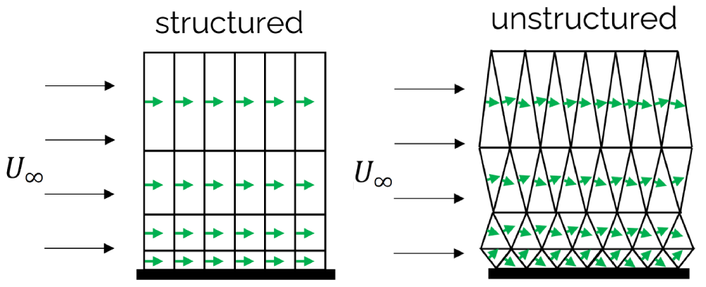
On the left side, we have some nicely stacked quad elements, growing in size away from the wall. Since the boundary layer will usually follow a solid wall (unless it is separating), the mean flow direction and the orientation of the surface normal vector are mostly aligned. If we contrast that with the triangular elements on the right, which have a similar spacing and growth away from the wall, we see misalignment between the mean flow and the surface normal vector, which becomes larger as we approach the wall.
This growing misalignment introduces false diffusion as we have seen above, which means that gradients in this region would be smoothed or dampened. However, we just said that we really want to have a really good prediction of our velocity gradient in this region to get an accurate drag prediction. Thus, we try to avoid triangles (2D) or tetrahedra (3D) near solid walls.
The solution is to use inflation layers. These offer a controlled way of wrapping a solid object in layers that ensure that most of the boundary layer flow is aligned with the surface normal vectors, resulting in low false diffusion and the best possible accuracy to predict the velocity gradient near walls. So if you ever wondered why you need inflation layers, this is the reason.
The question then becomes, how many layers do you need? Well, ideally, you want to capture the entire boundary layer. This is so that you capture the entire velocity profile. If you only had one inflation layer, you wouldn't capture the velocity profile well, and this would influence the computation of your velocity gradient near the wall. Conversely, if your entire velocity profile within the boundary layer is captured with inflation layers, you get a good velocity gradient and the best possible drag prediction.
As a rule of thumb, use 15-30 inflation layers if your target [katex]y^+[/katex] value is 1. If your target [katex]y^+[/katex] value is 30 or larger, start with 3-5 layers. These are experiential values, and they may differ for your specific case, but they give you a starting point to experiment with.
Aspect ratio
OK, we have now covered both the orthogonality and skewness quality metrics, which are arguably the most influential ones. In this section, I want to look at another important quality metric: the aspect ratio of a cell. It is somewhat detached from the skewness and orthogonality metric; that is, you can have a grid with no skewness and non-orthogonality, but still have a mesh containing high aspect ratio cells.
Let's look at the definition first. The general definition of an aspect ratio is the ratio of the largest to the smallest edge of a cell, as shown in the following figure:
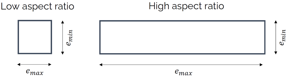
This works great for quad or hexa elements, but for triangles or tetrahedra we use a different definition. Here, we place two circles inside and outside the triangle. The inner circle will touch all edges of the triangle tangentially, while the outer circle will touch all vertices of the triangle. This is shown in the following figure:
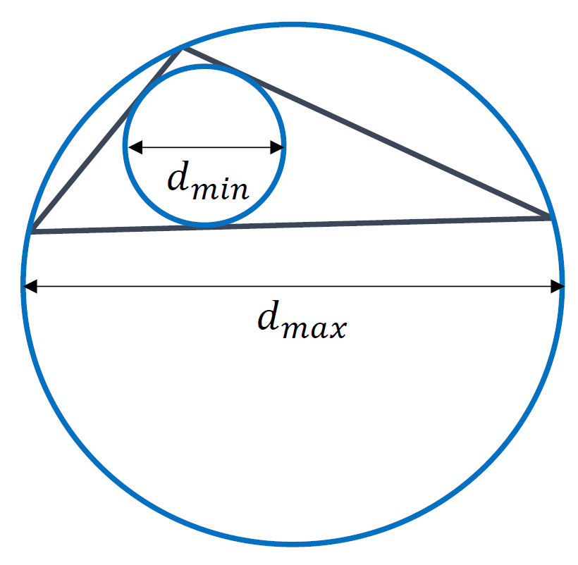
Thus, we can define the aspect ratio as:
Q_{aspect-ratio} = \frac{e_{max}}{e_{min}} = \frac{d_{max}}{d_{min}}\tag{19}This still only holds for quads and triangles, but we can generalise it. Instead of placing a circle around a given cell, as we did for the triangle above, we place a square (in 2D) or a cube (in 3D) around a cell, which fully encloses it. This square/cube is aligned with the coordinate axes. If you want, you can think of the square/cube as the axis-aligned bounding box (AABB).
Next, we compute the area/volume of the square/cube and the area/volume of the cell, which will be, by definition, smaller than or equal to the area/volume of its bounding square/cube. This is shown in the following figure, where we compute the aspect ratio of a general polygon in 2D, which is fully enclosed by a square. All vertices of the polygon touch the edges of the square:
Then, instead of using the edge length or diameter to compute the aspect ratio, we use the ratio of the areas or volumes of these two objects, i.e. we divide the square's/cube's volume by the cell's area/volume. We can write this as:
Q_{aspect-ratio}=\frac{A_{AABB}}{A_{cell}}=\frac{V_{AABB}}{V_{cell}}\tag{20}This works in 2D and 3D for any type of object. With this definition in mind, let's explore what some of the problems are with this definition. Imagine we are meshing an airfoil. We want to have [katex]y^+=1[/katex] everywhere, and we have a relatively large Reynolds number, say, above one million. This means that our first cell height will be orders of magnitude smaller than the chord length of the airfoil.
A common issue that we face, unless we take good care of our mesh, is that we get large aspect ratio cells at the trailing edge. If we don't set the spacing near the trailing edge equal to the first cell height, then we are going to get large aspect ratio cells near the trailing edge. This is schematically shown for the cells near the trailing edge of an airfoil:

Is this a problem? Well, let's increase the aspect ratio a bit and look at two cells in isolation, which meet at the trailing edge of the airfoil, as shown in the following figure:
A large aspect ratio may result in completely non-sensical values for the interpolated quantities at the cells' faces. We see that the blue arrow connecting both [katex]C_0[/katex] and [katex]C_1[/katex] intersects the face at a location which is not even on the face anymore. Clearly, whatever value we interpoalte to this location will not have much physical meaning.
The airfoil example is a good one, and, if you can generate a mesh and run that case on your machine, I would encourage you to do so. Most CFD solvers will struggle with this exact meshing issue (I have tried it in Fluent and OpenFOAM, and neither likes it). To avoid this, we could either:
- Reduce the spacing near the trailing edge to ensure we have an aspect ratio close to one (recommended)
- Connect both cells to another quad element that sits at the trailing edge where both cells connect. This avoids large deformation of cells at the trailing edge (and thus skewness) but also introduces a large area/volume ratio, which is the quality metric we will look at in the next section.
So, based on the airfoil example, we could say that aspect ratio alone is not a problem, only if we have skewness and non-orthogonality as well at play, do we get an issue, where interpolated values may not even be on the cells' faces anymore, right? Well, even for cases where there is no non-orthogonality and skewness do we get into trouble, potentially? Let's look at another example.
The following image depicts two grid arrangements. On the left, we have a Cartesian grid with no skewness, no non-orthogonality, and all cells have an aspect ratio of one. On the right, we see the same Cartesian grid, only now we have introduced some clustering, for example, to resolve the boundary layer near the bottom wall, which has led to an increase in the aspect ratio, while no additional skewness or non-orthogonality was introduced.
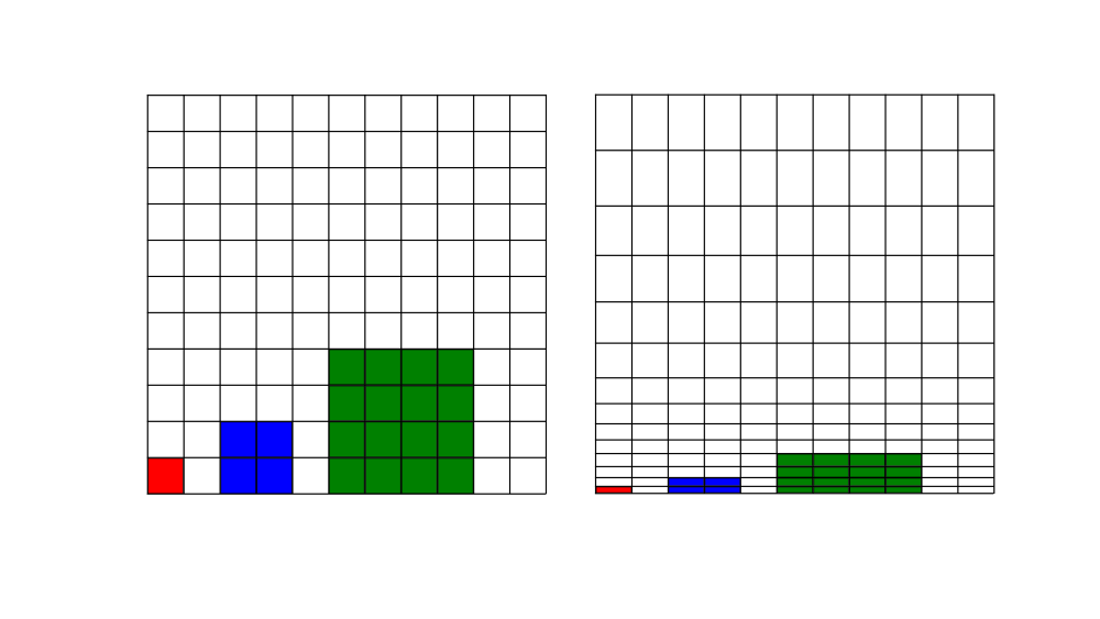
What I have also shown here is the cell sizes on a multigrid with three levels. If you have never heard of a multigrid before, think of it as a series of grids, which get coarser and coarser, on which we compute the solution. The advantage, in a nutshell, is that on the coarsest level, we typically only have a few hundred cells. Our simulation will converge pretty quickly on this grid, even if the full mesh has millions of cells.
After we have achieved convergence on the coarsest grid level (with a few hundred cells), we interpolate the solution onto the next finest grid level, perhaps with a few thousand cells. Since we already have an initial solution from the coarse grid, we don't have to iterate long to get a converged solution on this finer grid. This continues until we get down to the full grid.
If done correctly, a multigrid can be blisteringly fast and, for elliptic equations, nothing comes even close to how fast a multigrid operates. The pressure Poisson solver is an example of an elliptic equation, and for that reason, we like to use a multigrid for the pressure when dealing with incompressible flows, but with modifications, we can make the multigrid work for hyperbolic flows as well (e.g. compressible flows), but it is not as straight forward and requires some tricks to get working properly.
Back to the figure above, the cells shown in red, blue, and green indicate the size of our cells we would have on levels 0, 1, and 2 of our multigrid. That is, as we go from one level to the next, we combine cells together and their size increases.
One of the advantages of a multigrid is that by increasing the cell size, information can travel faster from one side of the domain to the other, and that is where it mostly derives its speed from. However, when we introduce high-aspect ratio cells, like we do in boundary layer flows, then even if we combine cells to make them larger for our multigrid, the cells on higher levels of the multigrid will still be rather small, at least if we compare the cells to those on a grid without hight aspect ratio cells.
If we look at the figure above again, I have given the same red, blue, and green cells on the right grid as well, where we have higher aspect ratio cells. We can see that the cells themselves are not as tall as the ones on the left grid, i.e. where we don't have any aspect ratio. Thus, high aspect ratio cells will decrease the efficiency of a multigrid solver, and thus increase the time it takes to get to a solution (computational cost is increased).
This isn't as much of an issue if we were to use something like a conjugate gradient method for the pressure, though in my experience, high aspect ratio or not, given the elliptic/parabolic and hyperbolic nature of the incompressible and compressible Navier-Stokes equations, respectively, there is very little in terms of performance gains between the conjugate gradient and multigrid approach.
I should also say that there will be opinionated CFD practitioners who will be deeply offended by that statement. For some, multigrid is a must, no matter what, and depending on your application, I can agree with that view. From a general view, though, whether the conjugate gradient or multigrid method is better suited for you will depend on your application.
Be that as it may, if we have the chance, we should try to avoid high aspect ratio cells. From experience, my observation is that once the aspect ratios get too large, your simulation will not converge anymore. Increase that aspect ratio a bit more, and your simulation will diverge. Some solvers are more resilient than others. For example, in Fluent, you may get away with aspect ratios that are of the order of one million, while OpenFOAM is known to struggle for anything that goes beyond an aspect ratio of 10,000.
As the saying goes (which I have just invented): Trashy mesh, no success. I rest my case.
Area/Volume ratio
The final mesh quality metric we want to look at is the area ratio (2D) or volume ratio (3D). The quality metric is rather straightforward and it quantifies how the area or volume changes between two subsequent cells, as shown in the following figure:
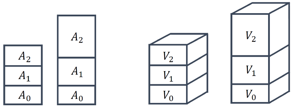
The area or volume ratio can then be computed as:
Q_{area-ratio} = \frac{A_1}{A_0}\\[1em]
Q_{volume-ratio} = \frac{V_1}{V_0}\tag{21}
By definition, we choose [katex]A_1[/katex] or [katex]V_1[/katex] to always be the largest of the two areas/volumes, and [katex]A_0[/katex] or [katex]V_0[/katex] to be the smallest of the areas/volumes. Thus, the area or volume ratio can never be smaller than 1 by definition, and it can only be larger than 1 if the areas or volumes differ.
This quality metric is much more straightforward to interpret compared to the other metrics. Take a look at the following airfoil simulation, for example, where we see the velocity magnitude on the left, and the magnitude of the velocity gradient tensor:
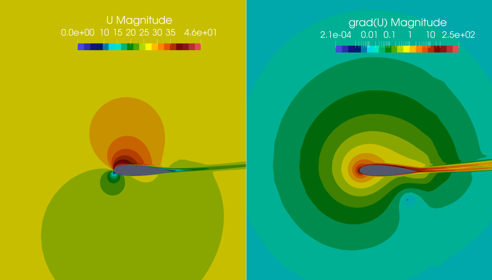
Here, I have used a log-scale for the contours on the right to show their variation a bit better. If I asked you to describe the variation of the contours, would you say these vary smoothly or abruptly? We can probably all agree that we have a very smooth variation. And this is something very typical for CFD applications. Even if we have shock waves or interfaces with a sharp discontinuity, these discontinuous changes are limited to small regions. Most of the domain will have smoothly changing variables in space.
Let's make this even simpler, let's just look at an xy plot, where we try to numerically approximate a given function (here shown by the solid black line):
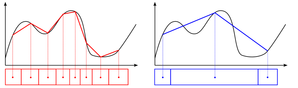
I have drawn two different grids here, one with a low area ratio (shown on the left, in red, below the plot) and one with a large area ratio (shown on the right, in blue, below the plot). If we assume we store values at cell centroids, as indicated by the dots, then we can find which values we would be storing in them, assuming we would be able to perfectly approximate the underlying function (shown in black). This is a strong assumption, but it won't change our discussion.
Because our variables in space change relatively smoothly, in general, we want to have cells without large jumps. As we can see on the right, once we introduce large area ratios, we jump over quite a bit of detail in our original function. If we look at the function we actually obtain by our numerical approximation, shown by the solid blue line on the right, it shows drastic deviations from the original function, shown in black.
However, by keeping the area ratio relatively small, as we can see on the left, the numerical approximation of the original function, shown by the solid red line, is much better compared to the blue line on the right. Thus, the main goal of keeping the area and volume ratio to a minimum is to enhance our predictive capabilities of gradients within our simulation.
And, just in case, to some it may appear obvious why we want to have a good gradient approximation (think, for example, back to our discussion on the skin friction and drag coefficient, which depend on the velocity gradient near the wall). However, there is an even stronger case for why we care about gradients so much. Have you seen this equation before?
\frac{\partial u}{\partial t} + u\frac{\partial u}{\partial x} = -\frac{1}{\rho}\frac{\partial p}{\partial x} + \nu\frac{\partial^2 u}{\partial x^2}\tag{22}Of course, you have, it is the Navier-Stokes momentum equation, here given in 1D. Each term is expressed as a derivative, and so if we want to find an accurate solution to this equation (which generally is what we try to do), we'd better make sure our gradients are approximated as accurately as possible.
See, I told you, this quality metric didin't take that much space to discuss, we have reached the end of the quality metric discussion. Next up, some best practices so you know if your mesh quality is "mediocre", "bad", "poor", "go home", or "perhaps CFD isn't right for you" (yes, this is the official quality scale, and yes, there is no such thing as a "good" mesh (unless you spend life on easy mode and only work with square Cartesian grids (but that's cheating! (please don't check my PhD thesis)))).
Mesh quality best practices
After we have gone through all of the definitions, we may know what all of these different quality metrics are, how they are defined, and what part of the simulation they influence. However, if we don't know what a sensible threshold is for each quality metric that we don't want to cross, then we may as well not bother at all with them.
So, in this section, I want to give you some of my best practices. These are the quality metric limits I typically try to achieve during meshing. These are not commandments set in stone but rather experiential values, as well as averaged limits gathered from various solver developers. Use these as a starting point, and adjust if your simulation is showing trouble converging.
The following tables show what the highest (ideal) value for our quality metric is. We typically only achieve these values on Cartesian grids without mesh refinement or other mesh deformation. For most practical applications, we want to ensure that we are within the acceptable quality metric column and avoid the poor quality metrics.
| Quality metric | Ideal quality metric | Acceptable quality metric | Poor quality metric (try again) |
|---|---|---|---|
| Orthogonality | 1 | 1 - 0.15 | [katex]\lt[/katex] 0.15 |
| Skewness | 0 | 0 - 0.85 | [katex]\gt[/katex] 0.85 |
| Aspect ratio | 1 | 1 - 10,000 | [katex]\gt[/katex] 10,000 |
| Area / volume ratio (boundary layers) | 1 | 1 - 2 | [katex]\gt[/katex] 2 |
| Area/volume ratio (boundary layers) | 1 | 1 - 4 | [katex]\gt[/katex] 4 |
If you are dealing with structured grids and you have a high Reynolds number, you might struggle getting below an aspect ratio of 10,000, especially if you have solid walls and want to have a low [katex]y^+[/katex] value. The trick is to have small aspect ratios in areas of strong gradients and put the high aspect ratio cells into areas of low gradients. This typically works quite well.
For the area and volume ratio, I have given two different definitions. Typically, within the boundary layer, we would like to achieve a growth rate of inflation layers (another way of expressing the area/volume ratio) that is not above 2. For academic applications, you will often find a value of 1.2, though for more complex cases, a value somewhere between 1.5 and 2 is a good compromise between accuracy and computational time.
For any other part of the mesh, e.g. the surface mesh and the far field, our area/volume ratio may be larger, and typically a value of 4 is acceptable. You may say this is a rather large value, and it is, but you will also find that if you create a mesh manually and you have to adjust spacings on complex geometries to get an acceptable area/volume ratio, a value of 4 can be difficult to achieve, or at least, it will require a lot of manual fine-tuning.
If you use an automatic mesh generation software, e.g. Fluent, StarCCM, OpenFOAM, ConvergeCFD, Numeca, etc., these will all try to create a mesh with acceptable area/volume mesh properties, so you don't really have to worry about this metric here. But if you create your mesh manual using Pointwise, ANSA, or Grid Pro (to name but a few), you will need to take care of that.
As mentioned before as well, check which way around your skewness is defined; it may be the opposite of how I defined it above. Because all other element metrics have an ideal value of 1, sometimes people like to say that a skewness of 1 is best and a value of 0 is worst, in which case the definition is flipped.
And, finally, if you ever face issues with mesh generation, there are only two things you can do to fix it:
- Spend more time on your mesh and optimise your mesh spacing and distribution. Typically requires some manual input on the mesh. If you don't have that, you can still resort to the second option
- Use more cells
In pretty much all cases where you have poor quality metrics, if you know where these are (in space), you can almost always get rid of these poor quality cells by just throwing more cells at the problem. You trade computational cost for grid quality. Remember the figure we looked at in the very beginning?
Better mesh quality is achieved by using more cells, or faster computations are achieved by reducing the mesh quality. Though if our mesh quality is getting too low, we may risk slowing down convergence, so we don't want to push our luck too much. In any case, mesh quality metrics are vital to any CFD simulation, and if you spend some time ensuring your mesh is free of poor-quality cells, you will have a much more enjoyable time simulating your case.
Mesh generation
Now that we have a good idea about mesh quality, we can finally tackle the mesh generation itself. In this section, we will look at structured and unstructured mesh generation techniques. But before we look into their details, let us first contrast these two different types of grids and understand their differences.
Structured vs. Unstructured mesh generation
There is often some confusion about the difference between structured and unstructured grids that I come across when talking with students and professionals. So I thought it would be good to show the differences here. The figure below shows a structured grid schematically:
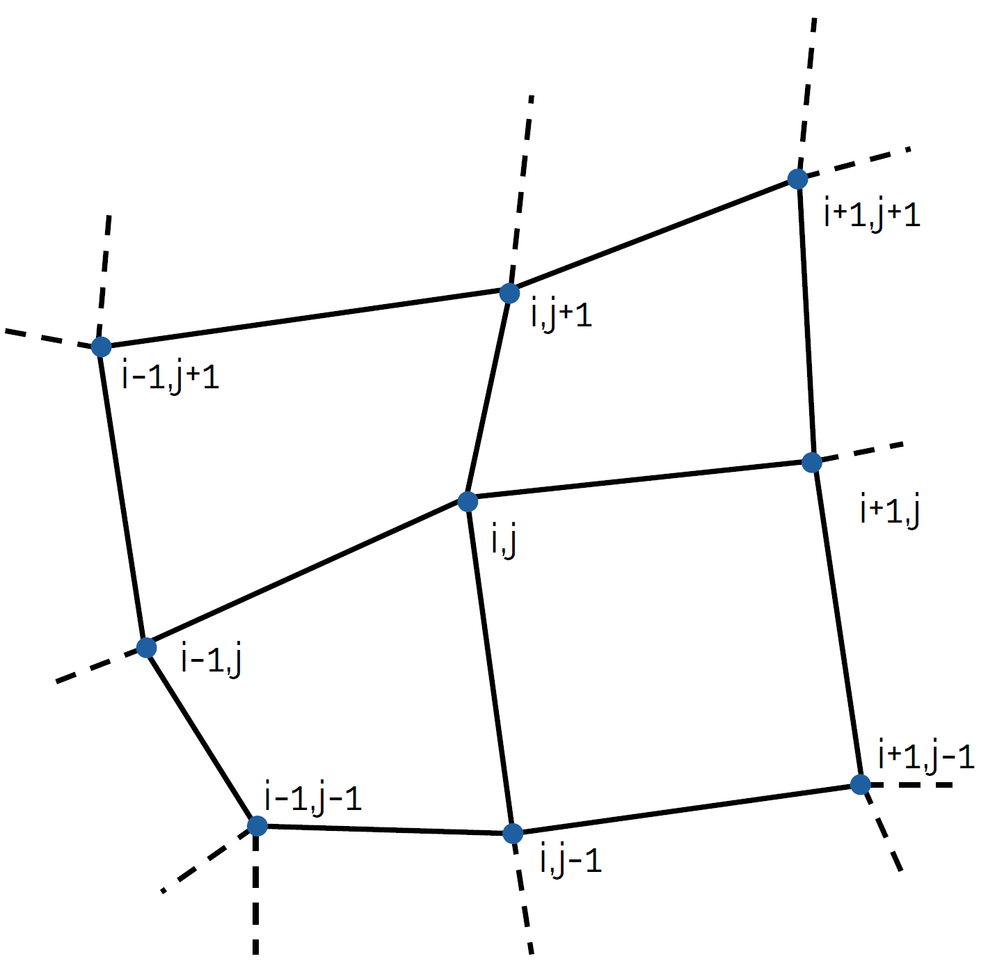
I have labelled vertices here by using [katex]i, j[/katex] indices, which are the indices we use to refer to specific vertices. The vertex in the centre is labelled [katex]i,j[/katex]. If I want to go to the vertex to the right, then I simply go to [katex]i+1,j[/katex]. If I want to go back from this vertex to the left, then I end up at [katex]i,j[/katex] again. I can do that as well for the vertices to the top ([katex]i,j+1[/katex]), to the bottom ([katex]i-1, j[/katex]), and to the left ([katex]i-1, j[/katex]). Regardless of which vertex I go to, I can always return to the vertex I started from.
In a mathematical sense, we could say that we have a bijective mapping, that is, for each vertex that maps to another vertex, there is a one-to-one mapping that allows me to go back to the original vertex. The power of this is that I can go to any vertex in the mesh, say, I could go to [katex]i+327, j-512[/katex], and I would always be able to go back to the original vertex (e.g. ([katex]i-327, j+512[/katex])).
Since our vertices are arranged in a structured way that allows us to index any other vertex in the mesh, we define these types of grids as structured grids. This requires that we can always go to the top, bottom, left, and right in 2D, and additionally to the front and back in 3D. This means we always have to have 4 directions in 2D, and 6 directions in 3D. The only elements that allow us to do this are quadrilaterals in 2D and hexahedra in 3D.
The image below shows an arrangement of an unstructured grid:
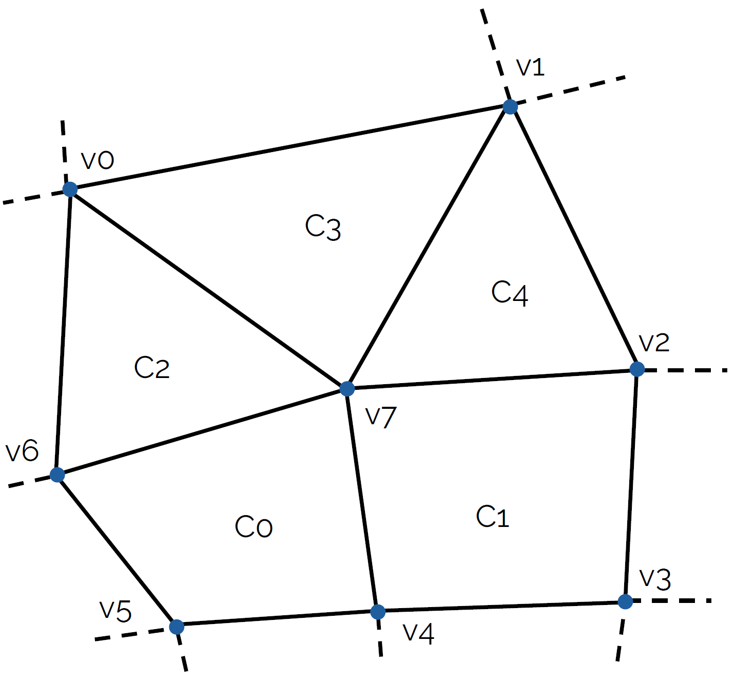
Unstructured grids have a different internal data structure compared to structured grids. To see why, let's place ourselves on vertex [katex]v7[/katex], i.e. the vertex located at the centre. Could we go down? Yes, we arrive at vertex [katex]v4[/katex]. Could we go up again and arrive at the same vertex? Yes, we would get back to [katex]v7[/katex]. This works because both [katex]v7[/katex] and [katex]v4[/katex] are part of a quad element.
However, if we want to go up, which vertex will we land on? We could go to either [katex]v0[/katex] or [katex]v1[/katex]. Let's say [katex]v1[/katex], for whatever reason, is the up direction. Now we are at [katex]v1[/katex], what is our down direction? Would we end up at [katex]v7[/katex] or [katex]v2[/katex]? The short answer is, we don't know; there is no clear mapping as there is for structured grids. The reason here is that we have used triangles, which only have three sides, and so they don't support an easy way to index to the top, bottom, left, and right.
Instead of indexing unstructured grids through their vertices, we typically define cells as we do in the figure above, e.g. [katex]C0[/katex], [katex]C1[/katex], [katex]C2[/katex], [katex]C3[/katex], and [katex]C4[/katex], and we store which vertices make up these cells. From that information, we can compute all relevant geometric information like the centroid, the volume, face areas, and face centroids. We also store connectivity information, for example, cell [katex]C0[/katex] is connected to cells [katex]C1[/katex] and [katex]C2[/katex].
Going back to our vertices, in a mathematical sense, we can say that we have a surjective mapping, that is, many vertices can map to the same vertex, and we have a many-to-one mapping. Don't get all mathematical on me, I know that many-to-one is not the definition of surjectivity, but it is a subset that applies here.
Completely irrelevant sidebar: In my first days at university as a fresh undergraduate student, we learned about bijective, injective, and surjective mappings, and our professor was, well, let's say not really motivated to teach this part of the lecture. This topic triggers me, still to this day, and back then, when I was fresh in university, I wrote a song about surjective, injective, and bijective images (as you do).
I went to look for it, but couldn't find it, however, I found another pearl instead, which I completely forgot about. After completing high school, I spent some time volunteering abroad instead of doing my military service (which was compulsory back then). I was living with two Italians who would randomly start to sing in the common area, and there was practically no soundproofing, so it felt like they were singing right next to me, in my room.
So I thought, their random performances needed to be recorded and archived for the next generations, and what better place to give them a platform and their 15 minutes of shame on a website that predominantly deals with CFD? (Hey, at least I try very hard to talk mostly about CFD). If you wonder what their angel-like voices sound like, here you go:
I forgot all about the burping, ah. That brings back memories ... Shall we move on?
Since we don't have a direct one-to-one (bijective) mapping of vertices, we have lost our structured way of indexing vertices, and thus we refer to these types of grids as unstructured grids. Unstructured grids can use any type of cell type, which makes them the de facto standard grid type we use in CFD. Especially for industrial applications, where we deal with complex geometries, unstructured grids reduce the effort to create grids to a minimum.
Structured grids preserve quality metrics better, i.e. we typically get good orthogonality and skewness values for them, regardless of how hard we try to create a really bad mesh. The biggest advantage of unstructured grids, namely that they can wrap around complex geometries, also becomes their largest liability, as it is very easy to generate a mesh with poor mesh quality metrics. Great care needs to be taken to ensure a high-quality mesh, and the burden here typically falls on the mesh generator developer.
The only reason structured grids have an edge over unstructured grids is their cell type. Quad and hexa elements are quality-preserving element types, you could say, and as long as you try to create a grid that maximises the orthogonality or reduces the skewness for these elements, you typically get a quite good mesh. Thus, a lot of effort has been put into developing unstructured algorithms that mimic structured grids, that is, introducing structured mesh components that bring back high-quality grids.
Typically, we see this in the form of a structured (Cartesian) background mesh that locally adapts to curvatures in geometry by placing a few triangles (2D) or tetrahedra (3D) between the Cartesian mesh in the far field and the mesh near solid boundaries, if there are any. A few mesh generators also introduced quad-dominant unstructured mesh generation algorithms, most commonly based on the advancing front method that we will look at later.
If we wanted to summarise structured and unstructured grids, how about the following pseudo set?
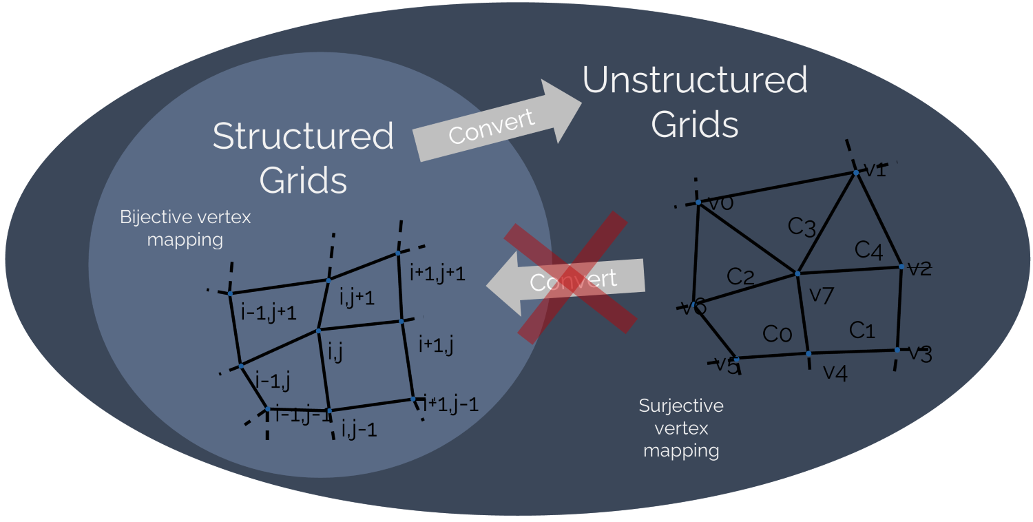
We see that the set of unstructured grids contains all structured grids. That is not to say that all structured grids are unstructured grids, but rather that all structured grids can be converted to unstructured grids (we can always define a cell based on its vertices). However, we cannot necessarily define a reverse mapping and convert an unstructured grid to a structured grid. In theory, though, for unstructured grids that only contain quad or hexa elements, we can find a reverse mapping, but this is the exception.
So, the difference between structured and unstructured grids is just how we represent them in the solver. Do we expose coordinates and [katex]i,j,k[/katex] indexing for the [katex]x[/katex], [katex]y[/katex], and [katex]z[/katex] directions? Or do we define cells that are made up of corresponding vertices, as well as some form of connectivity that tells us which cells are connected?
Just by looking at a grid, we can't say, and even if we know that we have a structured grid and load it into our solver, it may convert it to an unstructured grid, because the solver has been written to work with an unstructured data structure. Fluent is one such example, load in a structured CGNS file, and you can still run simulations, even though the solver is fully unstructured.
Don't be so quick to judge a mesh by its appearance. The only time when you can be certain that a mesh is unstructured is when it does not contain any quad or hexa elements. Even if there is a mix of quad and triangles, for example, it may be that we have a hybrid grid containing both structured and unstructured grid information (though I am not aware of any solver that would make use of that), as opposed to a mixed-element grid, which will be unstructured and contain a mix of element types.
Semantics, let's not get lost in them, let's go to structured grid generation and have a look at how we can get ourselves a nice, structured mesh, with really pristine quality metrics!
Structured mesh generation
Structured mesh generation can be split into two groups:
- Algebraic mesh generation
- Partial differential equation (PDE)-based mesh generation
We will look at both in this section, as well as coordinate transformation, a topic you can't avoid when dealing with structured meshes. But before we look at all those exciting partial differential equations, which I am sure you are dying to see, let's look at structured mesh topologies first and the necessity of the underlying blocking strategy.
Structured mesh topologies
The grids we can generate with structured meshes are categorised into 3 categories:
- O-grids
- C-grids
- H-grids
Combinations of these structured mesh topologies can be used as well. For example, for anything that involves circular shapes, you probably want to create a combination of an O- and H-grid. The classification of O-, C-, and H-grid stems from the shape the structured mesh is making, specifically, how the grid lines visually appear. Let us look at each type in turn to get a better idea.
O-grids
Let's imagine we want to generate the mesh around a square cylinder (you may call this simply a square, but CFD people have invented this new shape called a square cylinder, which is a square, not a cylinder. I didn't come up with it; I am just preaching the gospel. Don't shoot the messenger!). A grid around this geometry may look as follows:
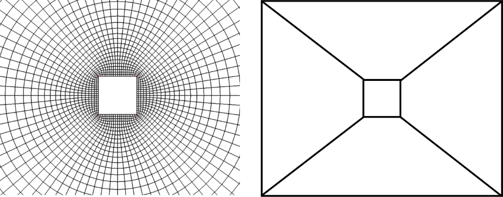
If we look at the shape of the grid lines that go around the square cylinder (in the circumferential direction), we see that these grid lines form the same shape as an O, and hence we refer to this shape as an O-grid. On the right of the figure, we see the blocking strategy we have to employ in order to get an O-grid. We have to generate 4 blocks, each of which will be meshed independently, and then we wrap them around our square cylinder and ensure that the edges of the block overlap.
We like to use O-grids to wrap geometries with a number of layers. These layers act as an inflation layer and ensure that we get good skewness near the wall (less numerical diffusion). Geometries that are actually circular, like a circular cylinder (you may call it just a cylinder, but not us CFD practitioners!), also benefit from O-grids, and these two scenarios are the most common use cases of where you would use an O-grid.
A giveaway sign for an O-grid is those diagonal lines in our blocking diagram, which we see on the right. If you are looking at a blocking diagram and you see diagonals within blocks, especially if these go around corners, then you will have an O-grid. We will see that in a second for a more complex example.
H-grids
Next up is the H-grid. An example is shown below:
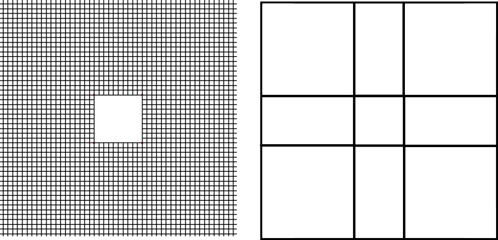
We can see that the grid lines are all nice and orthogonal to each other. In this example, it helps that the underlying geometry, i.e. the square cylinder, has itself orthogonal edges so that the mesh fits perfectly around. The blocking strategy we have to use to get an H-grid is shown on the right. We see that we need 8 blocks, which are all just stacked next to each other. No diagonals, just orthogonal edges everywhere.
Compare the grid that is generated with an O-grid and the H-grid; While the O-grid gives pretty good mesh quality everywhere, the H-grid provides no skewness and no non-orthogonality. Granted, it only works in this case because of the shape of the geometry, but there is one downside with the H-grid here. While for the O-grid we could specify essentially the first cell height, which would then be used around the entire geometry, the H-grid lacks a mechanism to enforce a uniform first cell height.
It is possible to have varying first cell heights around the object, and you may say, perhaps, that is a good idea. Even though you want to achieve a constant [katex]y^+[/katex] value around the object, the flow conditions will be different for all four edges of the square cylinder, and so we could use a different first cell height to keep the [katex]y^+[/katex] value roughly constant, right?
Well, yes, but then think about the corner points: we will now have two different first cell heights which meet at the corner point, and this could lead to an issue with eiother excessive aspect ratio and/or area/volume ratio cell arrangements, and this will bring related issues discussed in the aspect ratio and area/volume ratio quality metric sections.
At corner points, we probably have separated flow, and so we really want to have a high quality here, which we can easily assure with an O-grid. You could argue that you can probably get a high-quality mesh even with an H-grid here, and I would agree, but once the shapes become a bit more complicated, your H-grid will almost certainly always perform worse than an O-grid, especially if we have curvature.
The naming convention is also somewhat odd, don't you think? Instead of calling it an H-grid, I personally think we could have also called it an E, T, F, L, or X grid. Though I think there is an even better letter available, but we have to look beyond the English alphabet. In the Korean alphabet, the letter M is written as . If you ask me, the -grid (M-grid) would have been a much better choice, but no one asked me when they took a vote, and so I suppose we have to live with the name H-grid.
C-grids
The final topology we have available is the C-grid, and to some extent, it is a mixture of an O- and H-grid. Let's have a look at the following example:
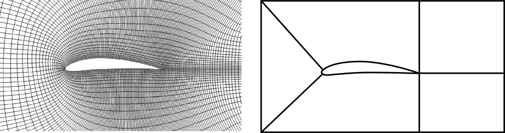
I dared to look beyond the square cylinder and increase the complexity; we are now dealing with an airfoil (exciting, I know!). Airfoils are pretty much the only use case for C-grids, even though we can apply them to other shapes as well. Just like the O-grid, we have some diagonals on one side, but then what resembles an H-grid on its opposite side. The mesh that is being generated looks like a C. From the blocking diagram, we can see that on the left side, we start to generate an O-grid, but on the right side, we switch to orthogonal edges instead of diagonal edges.
The reason we do that is to conform to shapes which have curvature on one side (e.g., the leading edge of an airfoil) and a singularity on the other side (e.g., the trailing edge of an airfoil). This pretty much describes the main characteristics of an airfoil, and hence the close connection between C-grids and airfoils. However, what happens if the trailing edge on the airfoil is blunt? In this case, the C-grid approach would struggle, if not fail, and this is a case where we need to combine two or more meshing strategies together.
Combinations of O-, C-, and H-grids
Let's go back to the square cylinder for a second and create a C-grid around it. We wouldn't want to do this in reality, as this would mess up the mesh quality, but as a thought experiment, let's do that. This mesh is shown in the figure below on the left.
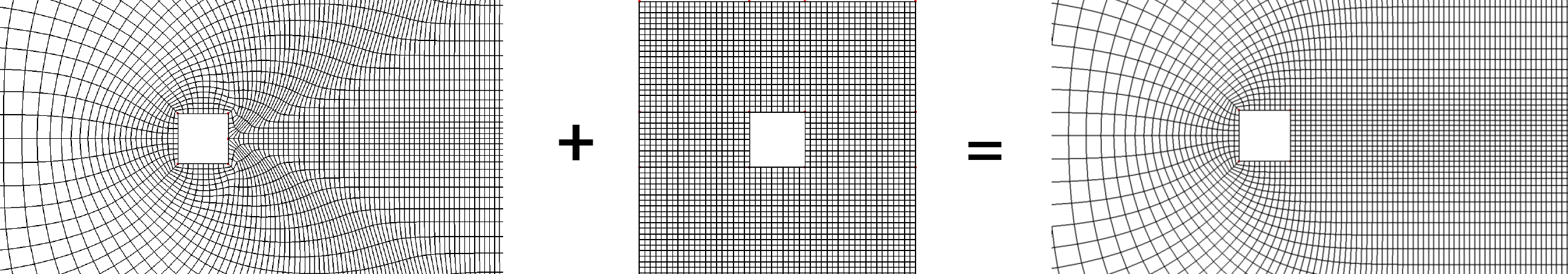
On the right side of the cylinder, the mesh has to awkwardly bend around the top right and bottom right corner points, just to reach the singularity on the right edge. This bending of the mesh will introduce non-orthogonality and skewness, and we probably would like to avoid this, given that we expect flow to separate here if it were coming from the left and going to the right.
So, what we can do is combine a C-grid with another blocking strategy, for example, an H-grid. Here, we would insert an H-grid where the wake of the cylinder would be, and then create a C-grid around the rest of the domain. This is shown schematically in the figure above. The resulting mesh shows a much better overall quality, especially in the wake region. Where we had highly skewed cells, we now have perfect orthogonality and no skewness.
The goal is always to increase the mesh quality, and knowing which type of combinations work well will take some experience and experimentation. If you ever have to create a structured grid, you will first need to think about your blocking strategy. The blocking strategy will make or break your structured mesh, so having an idea of how you want to create your mesh will take some thinking. But once that is done, mesh generation will become just a manual labour task that isn't difficult, but it may be time-consuming.
Let's have a look at a more complex example and develop the meshing strategy together.
Creating a blocking strategy for a complex example
Let's say we want to create a mesh around an aircraft. To practice the blocking strategy, let's look at a cross-section of the aircraft, showing the fuselage, wing, engine, and engine mount/pylon. The engine itself is empty, and we want to create a mesh inside here as well. Our task is to fill the entire domain with blocks that do not overlap. That is all.
It may seem simple at first, but once you sit down and try to do it yourself, you'll realise that the devil is in the detail. The following image shows how I would probably generate the blocks around this type of geometry, where the geometry (the aircraft) is highlighted in grey.
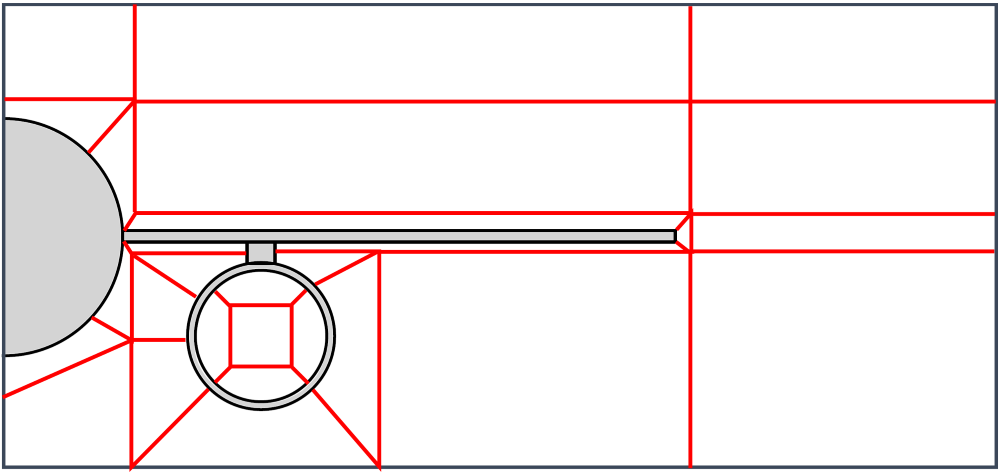
Let's examine the inside of the engine. Here, I have used a combination of an H-grid within the core fluid region, which is then surrounded by an O-grid so that we get high orthogonality near the engine walls. The fuselage is wrapped in an O-grid. Notice how we have only diagonal edges whenever blocks meet near the fuselage? This is the tell-tale sign of an O-grid. We do this, of course, to get nice inflation layers around the fuselage, to capture gradients accurately, so that we get a good estimate for our overall drag.
The outside of the engine is also meshed with an O-grid, again, to resolve the curvature without introducing low-quality elements here, as, for example, a pure H-grid would do. The rest of the far field is resolved using H-grids, pretty much. No need to overcomplicate things here; if we can use them, we may as well.
Even though I would consider myself an experienced mesh generation monkey (this is the official name given to someone generating grids predominantly, not by me, by people who use the words square cylinder to describe a square that isn't a cylinder), I tried a few blocking strategies before settling on the one you see above. It takes time to generate this figure, but the more time you spend on doing this, the easier your mesh generation process will be. Pen and paper are the best tools you can use in structured mesh generation!
One final word on grid topologies, which is often misunderstood by my students. We can only speak of O-, C-, and H-grids when we talk about structured grids. Sometimes I hear a student say, "I have used a C-shaped domain and an unstructured grid". This doesn't exist. The letters O, C, and H refer to the appearance of the grid lines, not the domain shape. Something to keep in mind: don't fall into the same trap.
Ok, so now that we know about these different grid topologies, we need to talk about how we can generate them. This is the task of algebraic mesh generators, which we will discuss in the next section.
Algebraic mesh generation
Algebraic mesh generation refers to the approach of taking simple grids, like meshed blocks, and making them fit around a body of interest. We have looked at the square cylinder for a while, so how about something else for a change? Let's look at the circular cylinder now. I know, my range of geometries I can recite is second to none!
The following figure shows schematically how algebraic mesh generation works in this example.

First, we have our geometry, i.e. the cylinder, and in this example, we want to take four meshed blocks and wrap them around the cylinder, i.e. we want to mesh it using an O-grid topology. This is shown on the left. The next step involves us moulding our blocks so that we can attach them together, like puzzle pieces, so that all edges of the blocks and the geometry (the cylinder) overlap.
In the process of moulding our blocks, we change the shape of our blocks, and so the internal grid of each block has to adjust. We use transfinite interpolation here, which is a process that makes sure that our grid lines will follow our boundaries. We will look at transfinite interpolation in the next section and see how it adjusts the internal mesh in response to changes in the edges of a block.
The final step is to adjust the mesh spacing. For example, if we actually wanted to simulate the flow around this cylinder geometry, we would probably want to resolve the boundary layer a bit better so that we capture gradients near the wall better. This would be driven by our [katex]y^+[/katex] requirements for turbulent flows. On the right in the figure above, we can see that some mesh clustering towards the wall was applied, and this would be the final step in our algebraic mesh generation approach.
In reality, we don't do all of the steps shown above separately, i.e. we don't create individual blocks and then later try to attach them together. Instead, we would already create all blocks in an attached state, according to our blocking strategy. But the takeaway point is that it is our job to first define the vertices of the block, then the edges, and then the mesh clustering on each edge, to create this algebraic mesh.
Some mesh generators have better support than others for this task, for example, ICEM-CFD from ANSYS is a pretty arcane mesh generator that, in theory, can be used for pretty much any mesh generation job, but its true power is in the generation of structured grids. It has a lot of features to make algebraic mesh generation as quick an affair as possible, though you will still be spending quite a bit of time to generate high-quality structured grids, especially in 3D.
Place yourself in the shoes of the pioneers who were advancing the field of CFD when it was still new in the 1950s and onwards. The computing resources that were available were steadily growing, and so we could simulate ever more complex geometries (and by complex, I mean cylinders and airfoils with grid sizes below 1000 cells!).
It became apparent that mesh generation was the part requiring the most manual input, and not much has changed until today; mesh generation still is one of the most time-consuming parts. This is not because mesh generation itself has not advanced since then; it has, significantly, but with an increase in computational power, doubling every 2 years since the 1970s, roughly (Moore's law), we wanted to simulate ever more complicated geometries.
Mesh generation advancements have not scaled the same way as Moore's law, but it became clear that manual mesh generation was not the future. Or would you like to mesh a full car, with all details, using a structured algebraic meshing approach? Enjoy drawing your blocking strategy for that on paper! No, we needed something more automated, and since unstructured grids were not a thing back then, people looked for ways to automate structured mesh generation.
People attempted to create equations that would generate the mesh based on some update process, and since the underlying equations we used were partial differential equations, we (creatively!) label this approach, wait for it, partial differential equation-based mesh generation. We will look at it as well in this section, but there are a few things we need to look at first.
First, we will look at transfinite interpolation, which is one missing piece we need to understand to finish our discussion on algebraic mesh generation. This is a pretty powerful method, which can be used not just to generate structured grids, but it also extends to 3D geometry generation as well, and you can create some quite complex 3D surfaces with this approach as well. So, let's look at that next.
Transfinite interpolation (TFI)
Transfinite interpolation is to algebraic structured mesh generation what grammar is to languages. Without it, we'd be lost in a sea of random words (cells) that form no coherent structure. Transfinite interpolation, or TFI, provides us with an automatic mechanism to take a block that has been meshed, transform the edges of the block, and then have the internal mesh within the block update as a response to the deformed edges of the block. It is automatic, and it doesn't require any input from us.
TFI is closely related to Coons patches, which is a type of parametric surface. Thus, if you understand what TFI is, you can write your own CAD program as well. Arguably, if you rely entirely on Coons patches, you lose out on a lot of flexibility of other types of parametric surfaces (i.e. Non-uniform Rational B-spline (NURBS) surfaces), however, the commercial mesh generator Pointwise can only create this type of surface, so Coons patches are powerful. �
To understand TFI (or Coons patches), there are a few things we need to first understand. Let's look at the following schematic first and then go through the different elements.
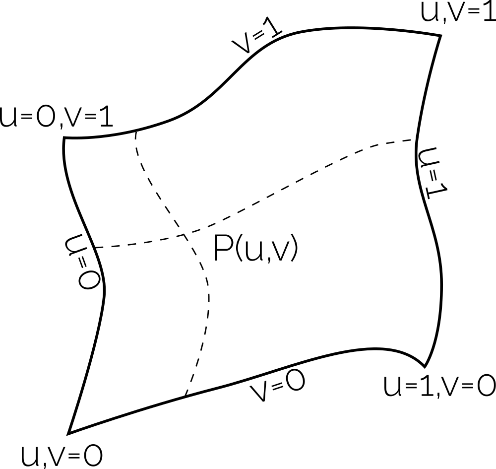
Here, we see an arbitrarily shaped 2D surface, which can be arbitrarily placed in 3D space. Each (Coons) patch, or surface on which we want to generate a mesh, has a [katex]u,v[/katex] coordinate system, which is local to each patch, and it goes from 0 to 1. We can find any point [katex]P[/katex] on the surface by giving some [katex]u,v[/katex] coordinate pairs, and we see that each edge will have either a constant [katex]u[/katex] or [katex]v[/katex] value of either 0 or 1.
To create our TFI, we need to define the edges of our patch first. This is done with so-called parametric curves. These are typically expressed as [katex]c(u)[/katex] or [katex]c(v)[/katex]. A general parametric curve can be expressed as:
c(u) = (1-u)P_0 + uP_1
\tag{23}
Here, [katex]P_0[/katex] and [katex]P_1[/katex] are two points, between which we would like to create the line. They can be in 1D, 2D, 3D, or even higher-dimensional space (though we typically limit ourselves to 3D). [katex]u[/katex] is again our non-dimensional coordinate that goes from 0 to 1, and we can understand Eq.(23) to be a linear interpolation between [katex]P_0[/katex] and [katex]P_1[/katex].
For example, let's say we have [katex]P_0=(1,5)^T[/katex] and [katex]P_1=(2,-1)^T[/katex]. Inserting a few values for [katex]u[/katex], we can compute what the value of the parametric curve should be:
| [katex]u=0.0[/katex] | [katex]u=0.2[/katex] | [katex]u=0.4[/katex] | [katex]u=0.6[/katex] | [katex]u=0.8[/katex] | [katex]u=1.0[/katex] | |
|---|---|---|---|---|---|---|
| [katex]c(u)[/katex] | 1.0, 5.0 | 1.2, 3.8 | 1.4, 2.6 | 1.6, 1.4 | 1.8, 0.2 | 2.0, -1.0 |
If we plot these values now, we see that they all fall onto a straight line. It is very similar to the classical formula for a line, i.e. [katex]y=mx+b[/katex], with the exception that we can apply Eq.(23) to any dimension.
Once we have identified all edges by a parametric curve, we are ready to apply the finite interpolation to it. The process is as follows:
- Create [katex](u,v)[/katex] coordinate for an undeformed Coons patch
- Define the four parametric curves that define the boundary of the deformed Coons patch
- Compute the correction the TFI needs to apply to map the undeformed [katex](u,v)[/katex] coordinates to the deformed Coons patch
- Compute the location in [katex](x,y)[/katex] space.
Steps 3 and 4 require us to compute the correction due to the TFI. Based on a current coordinate pair [katex](u,v)[/katex], we compute the point on the undeformed surface [katex]S[/katex] as:
S(u,v) = (1-v)c_{left}(u) + vc_{right}(u) + (1-u)c_{bottom}(v) + uc_{top}(v) - B(u,v)\tag{24}Here, the different curves [katex]c_{left}[/katex], [katex]c_{right}[/katex], [katex]c_{bottom}[/katex], and [katex]c_{top}[/katex] represent the parametric curves we have defined on the boundaries. At the end, we have a correction factor [katex]B(u,v)[/katex] that we need to apply, which is due to the TFI. This is computed as:
B(u,v) = (1-u)(1-v)P_{bottom,left} + u(1-v)P_{bottom,right} + (1-u)vP_{top,left} + uvP_{top,right}\tag{25}Here, [katex]P_{bottom,left}[/katex], [katex]P_{bottom,right}[/katex], [katex]P_{top,left}[/katex], and [katex]P_{top,right}[/katex] represent the corner points in our mesh. With this procedure, we can now compute the mesh on a deformed geometry. To make this clearer, let's look at an example.
In compressible flows, a classical test case to validate your solver is the inviscid bump example. In this case, we have a channel in which a little bump is located at the bottom wall in the centre. If the flow is inviscid, we expect the contour plot to show an almost symmetrical flow field, acknowledging that some flow separation at the rear will change the flow in the wake. The grid is shown in the following:
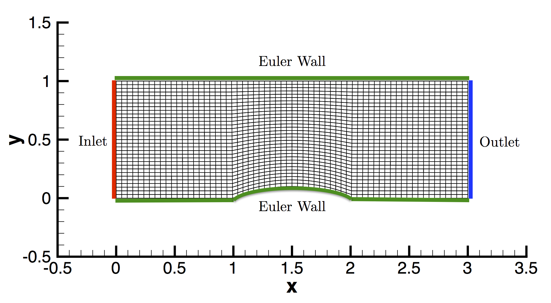
Let's say we want to create the mesh for this case using an algebraic mesh generation procedure, and we use the TFI here to generate the mesh in the centre part of the domain. This can be achieved with the following Python code:
import numpy as np
import matplotlib.pyplot as plt

# =============================================================
# STEP 1: Create (u,v) coordinate for an undeformed Coons patch
# =============================================================

# Define number of grid points for each block
n = 50

# Create uniform point distribution in horizontal direction
u = np.linspace(0, 1, n)

# Apply clustering in vertical direction using a power law
alpha = 2.5                         # strength of clustering
v_uniform = np.linspace(0, 1, n)
v = v_uniform**alpha                # non-uniform spacing in vertical direction

# Create meshgrid for (u,v) parameter space
U, V = np.meshgrid(u, v)

# ==============================================================================================
# STEP 2: Define the four parametric curves that define the boundary of the deformed Coons patch
# ==============================================================================================

# Define boundary curves
# Bottom curve: use sine wave to create hump
def C0(u):
    return np.array([u, 0.1 * np.sin(np.pi * u)])

# Top curve: straight line
def C1(u):
    return np.array([u, 1])

# Left curve: straight line
def D0(v):
    return np.array([0, v])

# Right curve: straight line
def D1(v):
    return np.array([1, v])

# Corner points
P00 = np.array([0, 0])
P10 = np.array([1, 0])
P01 = np.array([0, 1])
P11 = np.array([1, 1])

# Transfinite interpolation (Coons patch)
X = np.zeros_like(U)
Y = np.zeros_like(V)

for i in range(n):
    for j in range(n):
        u = U[i, j]
        v = V[i, j]

        c0 = C0(u)
        c1 = C1(u)
        d0 = D0(v)
        d1 = D1(v)

        # =========================================================================================================================
        # STEP 3: Compute the correction the TFI needs to apply to map the undeformed (u,v) coordinates to the deformed Coons patch
        # =========================================================================================================================

        B = (
            (1 - u) * (1 - v) * P00 +
            u * (1 - v) * P10 +
            (1 - u) * v * P01 +
            u * v * P11
        )

        # ===========================================
        # STEP 4: Compute the location in (x,y) space
        # ===========================================

        S = (1 - v) * c0 + v * c1 + (1 - u) * d0 + u * d1 - B

        X[i, j] = S[0]
        Y[i, j] = S[1]

# Plotting the TFI-transformed mesh
plt.figure(figsize=(8, 6))
for i in range(n):
    plt.plot(X[i, :], Y[i, :], 'k', linewidth=0.5)
for j in range(n):
    plt.plot(X[:, j], Y[:, j], 'k', linewidth=0.5)

# Plot boundary curves for clarity
u_vals = np.linspace(0, 1, 100)
bcurve = np.array([C0(u) for u in u_vals])
tcurve = np.array([C1(u) for u in u_vals])
lcurve = np.array([D0(v) for v in u_vals])
rcurve = np.array([D1(v) for v in u_vals])
plt.plot(bcurve[:, 0], bcurve[:, 1], 'k', linewidth=2)
plt.plot(tcurve[:, 0], tcurve[:, 1], 'k', linewidth=2)
plt.plot(lcurve[:, 0], lcurve[:, 1], 'k', linewidth=2)
plt.plot(rcurve[:, 0], rcurve[:, 1], 'k', linewidth=2)

plt.xlabel("X")
plt.ylabel("Y")
plt.gca().set_aspect('equal')
plt.tight_layout()
plt.show()I have done one small modification here. On lines 15-17, I have introduced a power-law to allow mesh clustering in the vertical direction. This means that I can allow for some clustering towards the bottom wall and thus resolve boundary layers better (well, we said it is an inviscid case, but we still have some flow separation, potentially, which we probably want to capture).
Setting a value for alpha that is larger than 1 allows for clustering to the bottom wall, and a value of less than 1 allows for clustering towards the top wall. Setting it to 1 will not use any clustering. If we run this code, we will generate the following meshed section for the bump region:
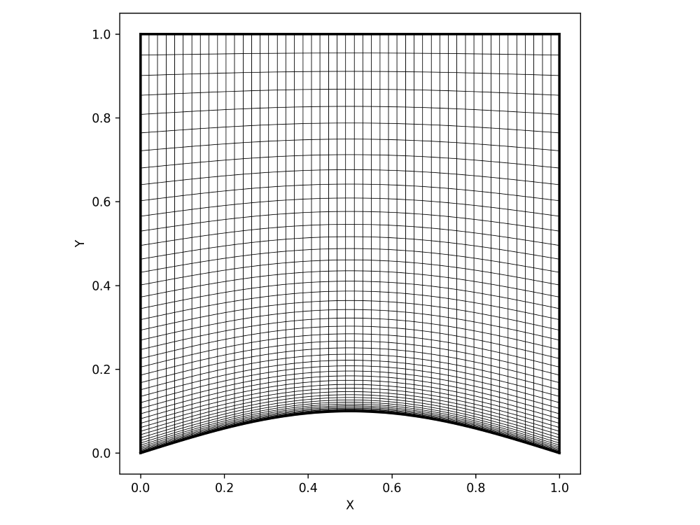
If you want to play around with it, start changing the shapes of the parametric curves between lines 28-41 and see what happens. You can also change the number of grid lines we use, i.e. n defined on line 9, and the clustering in the vertical direction by changing the value for alpha on line 15.
I think we have achieved a great deal here. With what you have learned in this section, you should be able to write your own structured mesh generators. Sure, for complex cases, you will need quite a bit of input, where a graphical user interface (GUI) would make sense, but obviously, that would also increase the complexity in terms of programming it.
However, if you want to write a bespoke mesh generator, say, for a wing or even just an airfoil, you should now have the tools you need to write these types of mesh generators. You only need to know how to define the parametric curves for airfoil shapes, which you can do by replacing the parametric curves with polynomials, and then use a polynomial function to represent airfoil shapes, such as the 4-digit NACA series.
With that, I want to leave the realm of algebraic structured mesh generation and look at the next important aspect of structured mesh generation: Coordinate transformations. Once we understand these, we can look at partial differential equation-based mesh generation.
Coordinate transformation
Why would we want to perform a coordinate transformation? Don't they make life more complicated? Yes and no. We need to put some mental effort into understanding what a coordinate transformation is, but once we understand it, and realise that it is just as complicated as remembering to put the bin out on a Friday (your bin day may vary). Plus, it is a one-time effort, i.e. before we start our simulation, we compute the coordinate transformation, store it, and then simply multiply it with our governing equation.
But why would we want to do it in the first place? Well, consider the following figure:
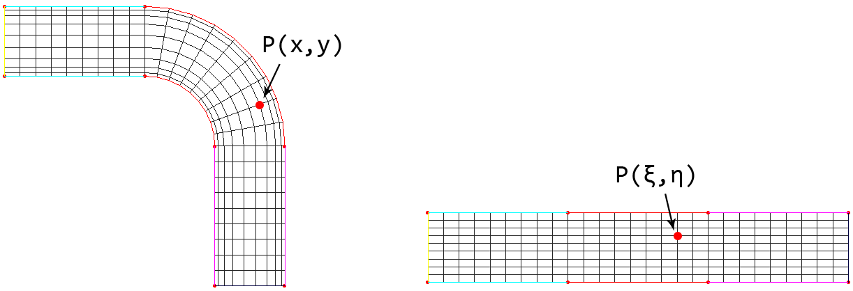
Here, we want to create a simple mesh around a bent channel shown on the left of the figure. Furthermore, we want to resolve gradients close to walls, so we employ mesh grading towards them. This will result in a mesh where distances between vertices will vary, and if we look at the orientation of the grid on the left, we see that our mesh is no longer aligned with our coordinate directions, and this will require special treatment when devising the numerical discretisation scheme.
If we are using the finite difference method, for example, we discretise our equations using a Taylor series, which in turn assumes that our grid is axis aligned and that grid spacings, e.g. [katex]\Delta x[/katex], [katex]\Delta y[/katex], and [katex]\Delta z[/katex], are constant. We could modify the Taylor series to allow variable spacings and arbitrary directions, and people have done that, but it turns out that this is more complicated (and thus slower) than using a coordinate transformation, so we don't use this approach.
Thus, transforming our mesh from the so-called physical space into the so-called computational space is a far more common approach. The transformation ensures that we end up with a structured and equidistant mesh spacing throughout our domain. That is, the transformed mesh will have [katex]\Delta \xi = const.[/katex], [katex]\Delta \eta = const.[/katex], and [katex]\Delta \zeta = const.[/katex], where [katex]\xi[/katex], [katex]\eta[/katex], and [katex]\zeta[/katex] are the new coordinates in the computational space, corresponding to the [katex]x[/katex], [katex]y[/katex], and [katex]z[/katex] coordinates in physical space.
In the figure above, we can see how the channel on the left in physical space is transformed to the geometry on the right in computational space, and we see how a single point on the mesh is transformed from one location to the other. We also see, in this 2D example, how we switch our coordinates from [katex]x[/katex] and [katex]y[/katex] to [katex]\xi[/katex] and [katex]\eta[/katex]. The requirement is that there is a one-to-one mapping from both spaces. If we do that, we can map any point, or vertex, from physical to computational space.
Here we go again, we have a bijective mapping ...
One of the advantages of the coordinate transformation is that it not only applies to the finite difference method, but we can apply it to the finite volume method just as well. If we go with a finite volume approach, we probably want to use an unstructured grid, in which case, we really don't need any mesh transformation, but you may have a special use case in mind.
Perhaps you want to solve the compressible Navier-Stokes equations for high-speed flows, those that include shocks. You pretty much always want to use the finite volume method here. Then, when it comes to mesh generation, you don't need a sophisticated mesh generation algorithm, so you are content with generating block-structured grids with your solver. Perhaps you want to have mesh clustering towards the wall, as we did in the channel with a bump example above, when talking about transfinite interpolations.
In cases like these, you can apply a coordinate transformation as well. Even though we originally introduced it to extend the finite difference method to include more complex (curvelinear) structured grids, we can just as well introduce it to other discretisation frameworks and benefit from simplified discretisations.
In the finite element method, for example, coordinate transformations are used all the time and are known as isoparametric mappings, typically used in conjunction with Lagrangian shape functions. These shape functions are defined on so-called reference or standard elements, and we need to map those shape functions onto elements in our grid. I remember having to implement this for a compressible solver on an unstructured grid, oh what joy overcometh my heart ...
The question then becomes, how do we transform from one coordinate system into another? Let's build up an intuitive understanding of this with an example. Say you have two maps, one which shows the details of a neighbourhood and one which shows the entire city. The map, which shows the neighbourhood, also has a grid, so you can easily measure distances. This is schematically shown in the following:
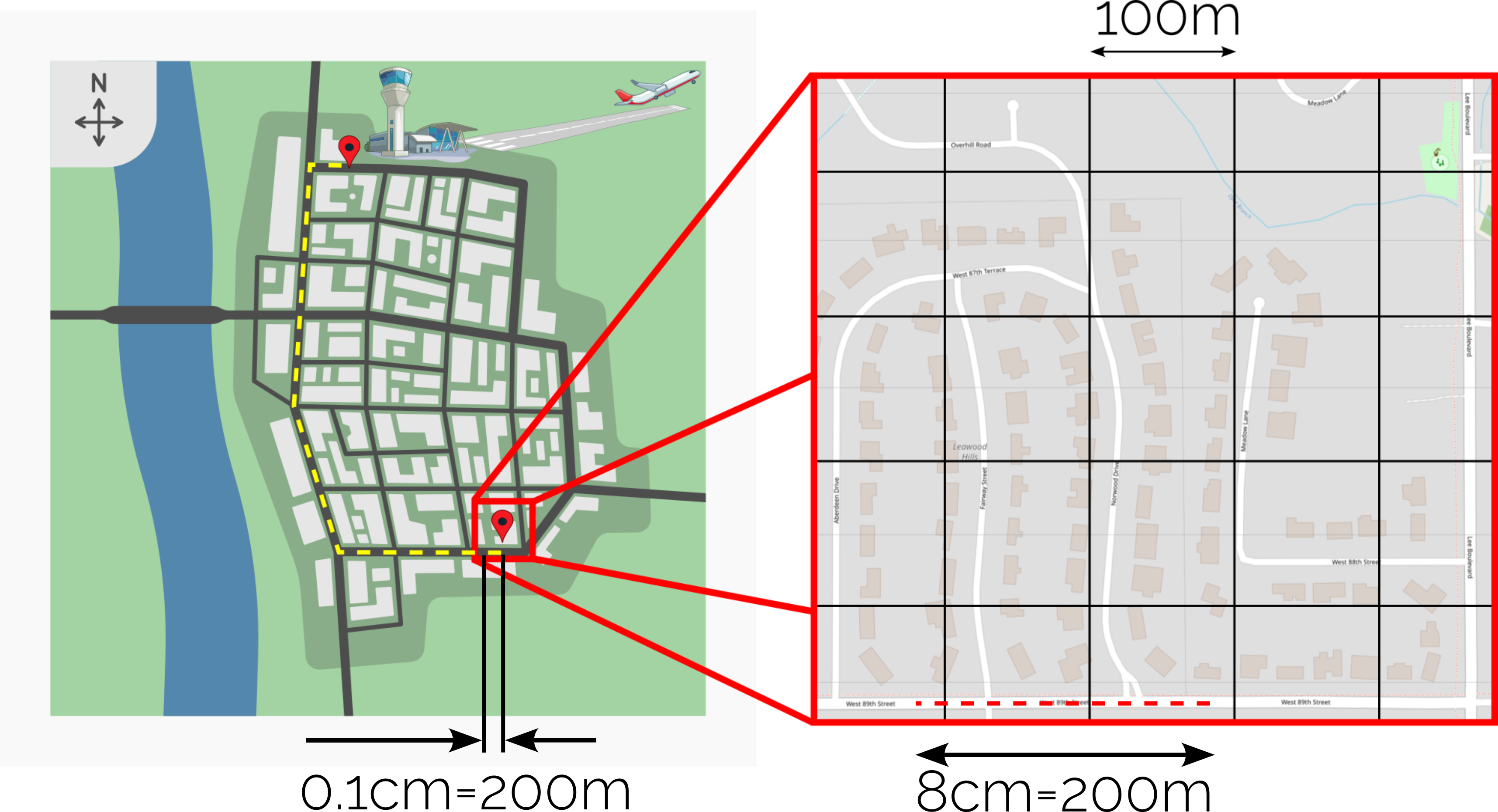
Let's say this is in the dark ages (i.e. 1990, with the internet essentially non-existing), so there is no Google Maps and the like. GPS may have existed for military applications, but not for n00bz like me and you (I doubt I would have had any use for GPS in 1990, I was still pooping in dipers, as I said, the dark ages ...). But let's assume we wanted to go from our location in the neighbourhood, for which we have a detailed map, to, say, the airport.
We can find a simple path from our location to the airport, but now we want to know how long it would take us to go from our house all the way to the airport. We know that on a normal day, we can drive at 50 kph, or 30 mph, so if we know the distance, we can compute a time using time = distance / speed. So, how would we go about this?
We could argue that a sensible approach would be to measure a distance in the map on the right, where we can determine the distance for a small part of the journey with relatively high precision. Let's say we measure the distance with a ruler on the map on the right between grid lines, and we measure that these grid lines are 4 centimetres apart. We know that the distance is 100 meters on the map. Now we find a part of our journey that we can measure in both maps, which is inside the red rectangle.
Let's measure the red dashed line on the right map and say it is a distance of 8 centimetres on the map, which means that the real distance would correspond to 200 meters. Let's say that the same distance measured on the map on the left is only about 0.1 centimetre. This means that, for the map on the right, we can say that 1 centimetre of measurement corresponds to 25 meters (200 / 8), while 1 centimetre in the map on the left corresponds to 2000 meters, or 2 kilometres (200 / 0.1). Therefore, the scale is 1:80 (25 / 2000).
We can use this now to measure the distance from our location to the airport. Say the yellow dashed line is a distance of 100 centimetres. Then, we multiply this value by 80 to get the distance in meters. In this case, 100 times 80 gives us 8000 meters, or 8 kilometres. With a speed of 50 kph (kilometres per hour), we'll be at the airport in about 10 minutes, assuming no red lights, crashes, or bank heists on the way.
But what happens if I give you a different map with a different scale, and you have to work this out again? You may be interested in coming up with an equation that can compute distances based on the map scale. Let's try to come up with a generic equation:
d(map_B)\cdot scale = d(map_A) \\[1em]
d(map_B)\cdot (1:80) = d(map_A) \\[1em]
d(map_B)\frac{1}{80} = d(map_A)\tag{26}
Easy enough, we introduce a simple mapping in which we say that the distance [katex]d[/katex] on [katex]map_B[/katex], for example, the map on the left in the figure above, can be expressed by knowing a distance [katex]d[/katex] and a different [katex]map_A[/katex], for example, the map on the right in the figure above, as well as the scale between [katex]map_A[/katex] and [katex]map_B[/katex]. We have hardcoded the scale here, but in reality, we would like this to be more generic. We could write the scale as
scale = \frac{\Delta s_B}{\Delta s_A}
\tag{27}
Here, [katex]\Delta s_A[/katex] and [katex]\Delta s_B[/katex] are the distances we measure in each map. In our example, we had [katex]\Delta s_B=0.1[/katex] and [katex]\Delta s_A=8[/katex]. This would result in a scale of 1:80 in Eq.(27). However, we could have also set [katex]\Delta s_B=10^{-10}[/katex] and then check what [katex]\Delta s_A[/katex] would be.
We would see that the ratio is always constant, regardless of what we set for [katex]\Delta s_B[/katex]. So, we will always get that [katex]\Delta s_A[/katex] is 80 times larger than [katex]\Delta s_B[/katex]. So, by making the ratio infinitely small, we can replace the differences by differentials and we get:
scale = \frac{\mathrm{d}s_B}{\mathrm{d}s_A}
\tag{28}
For a constant change in [katex]s_B[/katex], how much does [katex]s_A[/katex] change? This is all that this equation expresses. Now, let's try to bring that back to our coordinate transformation. First of all, instead of using variables [katex]s_B[/katex] and [katex]s_A[/katex] here, let's say that distances measured on [katex]map_B[/katex] (on the right) are expressed now as [katex]x[/katex], and distances measured on [katex]map_A[/katex] are expressed as [katex]\xi[/katex]. Then, we can rewrite Eq.(28) as:
scale = \frac{\mathrm{d}x}{\mathrm{d}\xi}
\tag{29}
We could also express it as the inverse (which we will use later):
scale = \frac{\mathrm{d}\xi}{\mathrm{d}x}
\tag{30}
We do that as we really want to take a measurement in [katex]x[/katex], but this is difficult, so we make measurements in [katex]\xi[/katex] and then translate how these measurements relate to measurements in [katex]x[/katex]. This is the same in CFD and our coordinate transformation. We want to simulate our flow in physical space, i.e. [katex]x[/katex], but this is difficult (mesh deformation, variable mesh spacing), so instead, we simulate everything in computational space, i.e. [katex]\xi[/katex], and then translate these results back into physical space, i.e. [katex]x[/katex].
The Navier-Stokes equations are expressed as differential, specifically, partial differentials, but the same idea can be applied here. For example, let's take the 1D, incompressible continuity equation, to make things simple. In physical space, we can write:
\nabla\cdot \mathbf{u}=\frac{\partial u}{\partial x}=\frac{\partial}{\partial x}u = 0
\tag{31}
This example is a bit more complicated compared to the map example, because we have to deal now with partial differential equations. However, forget for a moment that we are dealing with Navier-Stokes, and just focus on what we want to do: all we want is to transform Eq.(31) from physical space ([katex]x[/katex]) to computational space ([katex]\xi[/katex]).
This means we want to express our derivatives with respect to [katex]\xi[/katex], not [katex]x[/katex], and to do this, we need to introduce our scaling factor, i.e. Eq.(30), to translate gradient measurements from one coordinate system to the other. We can express this as:
\frac{\partial}{\partial \xi}\frac{\partial \xi}{\partial x}u = 0 \\[1em]
\frac{\partial \xi}{\partial x}\frac{\partial}{\partial \xi}u = 0 \\[1em]
\frac{\partial \xi}{\partial x}\frac{\partial u}{\partial \xi} = 0\tag{32}
This almost looks like what we want. We evaluate now our gradient of [katex]u[/katex] with respect to [katex]\xi[/katex], which is great, but let's look at [katex]\partial \xi/\partial x[/katex], which is also referred to as the metric coefficient, or just metric. We evaluate the gradient of [katex]u[/katex] with respect to [katex]\xi[/katex], but the metric term is evaluated with respect to [katex]x[/katex]. This means we have to evaluate these two terms in different coordinate systems.
Ideally, we would like to have an inverse metric coefficient here, as in:
\frac{\partial x}{\partial \xi}\frac{\partial u}{\partial \xi} = 0 \\[1em]
x_\xi \frac{\partial u}{\partial \xi} = 0\tag{33}
Here, I have introduced the shorthand notation for the metric coefficients that we often see in the literature. That is, a partial derivative [katex]a[/katex] that is differentiated with respect to [katex]b[/katex] can be written as [katex]a_b[/katex], or [katex]\partial x/\partial \xi[/katex] becomes [katex]x_\xi[/katex].
The beauty of this transformation is that even though we may have a curvelinear grid, i.e. we have a structured grid that is arbitrarily deformed in 3D space, in computational space, all grid lines are straight and aligned with the computational space's coordinate system. Furthermore, while in physical space we don't necessarily have [katex]\Delta x=const.[/katex], in computational space, [katex]\Delta\xi=const.[/katex] is always given. Even better, we can arbitrarily choose what value [katex]\Delta\xi[/katex] should be.
If we set [katex]\Delta\xi=0.5[/katex], for example, and we discretise our continuity equation with a central scheme, then we get:
x_\xi \frac{\partial u}{\partial \xi} \approx x_\xi \frac{u_{i+1}-u_{i-1}}{2\Delta\xi}=x_\xi \frac{u_{i+1}-u_{i-1}}{1}=x_\xi(u_{i+1}-u_{i-1})\approx 0\tag{34}In our discretised equations, it is possible that approximate partial derivatives reduce to simple differences, based on our choice of [katex]\Delta\xi[/katex]. And, just in case you find it strange that I say we can set [katex]\Delta\xi[/katex] arbitrarily, if we change [katex]\Delta\xi[/katex], then [katex]x_\xi[/katex] changes in the same proportion, so that the product of the two remains constant.
But think about it. We determine the coordinate transformation, and we can make the computational grid as small or large as we want. Bringing that back to our map example, we could have taken a much smaller map or a much larger map. The distance that we measured on the smaller map would now be completely different. Instead of measuring 8 centimetres, for example, we may measure 2 centimetres or 16 centimetres.
It doesn't matter, though, because the scale would also change. If the measurement was 2 centimetres, then the scale would be 1:20, and if it was 16 centimetres, the scale would be 1:160. We saw that the scale is essentially our [katex]x_\xi[/katex] variable, so changing the map size (or the grid in computational space, i.e. [katex]\Delta\xi[/katex]) will not make a difference to our transformation.
Let's generalise this idea. So far, we have only looked at a 1D example to keep things simple. But let's dare to look at what a 2D example would look like. So, for the 2D continuity equation, we have:
\nabla\cdot\mathbf{u}=\frac{\partial u}{\partial x} + \frac{\partial v}{\partial y} = 0\tag{35}So now we also have the [katex]y[/katex], and thus [katex]\eta[/katex] coordinate direction to contend with. You might assume that the following transformation would be suitable:
\frac{\partial}{\partial \xi}\frac{\partial \xi}{\partial x}u + \frac{\partial}{\partial \eta}\frac{\partial \eta}{\partial y}v = 0
\tag{36}
Under very specific circumstances, this transformation holds, but it is not a general transformation relation. Why, you may ask? Well, remember that [katex]x_\xi[/katex] essentially is a mapping from one coordinate system to another, and it tells us by how much we are changing, like the scale in the map example. But if I deal with an arbitrarily deformed mesh in physical space, where the grid is not necessarily aligned with the physical space's coordinate system, then things change.
For the sake of argument, let's assume at one point in the grid, a specific grid line connecting two vertices is at a [katex]45^\circ[/katex] angle with the x-axis. Thus, if we make changes in [katex]x[/katex], i.e. we go from one vertex to the other, there is not just a change in [katex]x[/katex], but also in [katex]y[/katex]. Thus, when we go from one coordinate system to the other, we have to check each coordinate direction and transform all possible changes. Eq.(36) can be generalised as:
\underbrace{\frac{\partial}{\partial \xi}\frac{\partial \xi}{\partial x}u + \frac{\partial}{\partial \eta}\frac{\partial \eta}{\partial x}u}_{\text{change in }x} + \underbrace{\frac{\partial}{\partial \xi}\frac{\partial \xi}{\partial y}v + \frac{\partial}{\partial \eta}\frac{\partial \eta}{\partial y}v}_{\text{change in }y} = 0 \\[1em]
\underbrace{\xi_x\frac{\partial u}{\partial \xi} + \eta_x\frac{\partial u}{\partial \eta}}_{\text{change in }x} + \underbrace{\xi_y\frac{\partial v}{\partial \xi} + \eta_y\frac{\partial v}{\partial \eta}}_{\text{change in }y} = 0
\tag{37}
We can also write this in the shorthand notation that we introduced previously, which results in:
\underbrace{\xi_x\frac{\partial u}{\partial \xi} + \eta_x\frac{\partial u}{\partial \eta}}_{\text{change in }x} + \underbrace{\xi_y\frac{\partial v}{\partial \xi} + \eta_y\frac{\partial v}{\partial \eta}}_{\text{change in }y} = 0\tag{38}If we wanted to extend this to 3D, we could. This would result in:
\underbrace{\xi_x\frac{\partial u}{\partial \xi} + \eta_x\frac{\partial u}{\partial \eta} + \zeta_x\frac{\partial u}{\partial \zeta}}_{\text{change in }x} + \underbrace{\xi_y\frac{\partial v}{\partial \xi} + \eta_y\frac{\partial v}{\partial \eta} + \zeta_y\frac{\partial v}{\partial \zeta}}_{\text{change in }y} + \underbrace{\xi_z\frac{\partial w}{\partial \xi} + \eta_z\frac{\partial w}{\partial \eta} + \zeta_z\frac{\partial w}{\partial \zeta}}_{\text{change in }z} = 0
\tag{39}
From Eq.(39), we can try to generalise the transformation relation as follows:
\frac{\partial}{\partial x} = \frac{\partial}{\partial \xi}\frac{\partial \xi}{\partial x} + \frac{\partial}{\partial \eta}\frac{\partial \eta}{\partial x} + \frac{\partial}{\partial \zeta}\frac{\partial \zeta}{\partial x} = \xi_x\frac{\partial}{\partial \xi} + \eta_x\frac{\partial}{\partial \eta} + \zeta_x\frac{\partial}{\partial \zeta} \\[1em]
\frac{\partial}{\partial y} = \frac{\partial}{\partial \xi}\frac{\partial \xi}{\partial y} + \frac{\partial}{\partial \eta}\frac{\partial \eta}{\partial y} + \frac{\partial}{\partial \zeta}\frac{\partial \zeta}{\partial y} = \xi_y\frac{\partial}{\partial \xi} + \eta_y\frac{\partial}{\partial \eta} + \zeta_y\frac{\partial}{\partial \zeta} \\[1em]
\frac{\partial}{\partial z} = \frac{\partial}{\partial \xi}\frac{\partial \xi}{\partial z} + \frac{\partial}{\partial \eta}\frac{\partial \eta}{\partial z} + \frac{\partial}{\partial \zeta}\frac{\partial \zeta}{\partial z} = \xi_z\frac{\partial}{\partial \xi} + \eta_z\frac{\partial}{\partial \eta} + \zeta_z\frac{\partial}{\partial \zeta}
\tag{40}
So, if we have the continuity equation in 3D, given as:
\frac{\partial}{\partial x}u + \frac{\partial}{\partial y}v + \frac{\partial}{\partial z} w = 0 \tag{41}Then, we can insert Eq.(40) for [katex]\partial/\partial x[/katex], [katex]\partial/\partial y[/katex], and [katex]\partial/\partial z[/katex], which would result in Eq.(39). Thus, Eq.(40) is the general transformation relationship we can apply to transform from computational into physical space.
Depending on how much you remember from calculus, you may realise that we are simply using the chain rule here. And this is the secret to coordinate transformations! Well, with the small exception that I said we really want to have the inverse transformation, rather than the one we see above. That is, instead of evaluating our metric coefficients with respect to the physical space ([katex]x[/katex], [katex]y[/katex], [katex]z[/katex]), we want the inverse mapping so that all metric coefficients are evaluated in computational space ([katex]\xi[/katex], [katex]\eta[/katex], [katex]\zeta[/katex]).
That is, all metric coefficients given above, i.e.:
\xi_x \quad \eta_x \quad \zeta_x \quad \xi_y \quad \eta_y \quad \zeta_y \quad \xi_z \quad \eta_z \quad \zeta_z\tag{42}Should be expressed as:
x_\xi \quad x_\eta \quad x_\zeta \quad y_\xi \quad y_\eta \quad y_\zeta \quad z_\xi \quad z_\eta \quad z_\zeta \quad \tag{43}To do that, we need to figure out how we can invert our metric coefficients. We'll stay in 2D, as this will make my life easier, coming up with an example that we can intuitively understand, but the same discussion below holds for 3D as well. To invert our metric coefficients, we will need the so-called total differential, so let's see what it represents and how we can interpret it.
Let's assume we are hiking on a mountain. We are hiking in a north-east direction, and we want to know how much our elevation has changed for a small portion of our hike. If we only know, from maps, for example, how the elevation changes separately in the north and east direction, then we can simply add these changes together, that is:
\text{total elevation change} = \text{east elevation change} + \text{north elevation change}\tag{44}Let's say that the east-west direction is expressed as the [katex]x[/katex] direction, and the north-south direction is expressed as the [katex]y[/katex] direction. We measure the change in elevation over some distance, and then compute the average change over [katex]1[/katex] meter in the north and east direction. This change, per meter, is a gradient. So if the elevation change is [katex]0.1[/katex] meters for every meter we walk, then the gradient at that point is [katex]0.1/1=0.1[/katex]. If we now know the total distance hiked in the north and east direction, we can rewrite our equation as:
\text{total elevation change} = \text{east elevation change per 1 meter}\cdot\text{east distance travelled} + \\
\text{north elevation change per 1 meter}\cdot\text{north distance travelled}\tag{45}
Now, since none of us are doing management, or marketing, or supply chain management, we can dare to express the equation above more mathematically. Let's say that the elevation is expressed with the letter [katex]E[/katex], it's change per 1 meter is a gradient expressed as [katex]\partial E/\partial x[/katex] or [katex]\partial E/\partial y[/katex] in the east and north direction, respectively, and the distance travelled in the east and north direction is expressed as [katex]\mathrm{d}x[/katex] and [katex]\mathrm{d}y[/katex], respectively. Then, we get:
\mathrm{d}E = \frac{\partial E}{\partial x}\mathrm{d}x + \frac{\partial E}{\partial y}\mathrm{d}y\tag{46}Here, I am using [katex]\mathrm{d}E[/katex] to state that we are expressing a difference in elevation, i.e. by how much does the elevation change from one point to another. We could extend this to 3D space by adding [katex](\partial E/\partial z)\mathrm{d}z[/katex]. For our hiking example, though, this would not work, so we just use a 2D space here.
In any case, we can apply this equation now to something more generic. In our particular case, we want to know how [katex]\xi[/katex] and [katex]\eta[/katex] change as we go through our grid in physical space, i.e. in the [katex]x[/katex] and [katex]y[/katex] direction. This is shown in the following equations:
\mathrm{d}\xi = \frac{\partial \xi}{\partial x}\mathrm{d}x + \frac{\partial \xi}{\partial y}\mathrm{d}y = \xi_x\mathrm{d}x + \xi_y\mathrm{d}y \\[1em]
\mathrm{d}\eta = \frac{\partial \eta}{\partial x}\mathrm{d}x + \frac{\partial \eta}{\partial y}\mathrm{d}y = \eta_x\mathrm{d}x + \eta_y\mathrm{d}y
\tag{47}
Eq.(47) is known as the total differential of [katex]\xi[/katex] and [katex]\eta[/katex]. Here, instead of measuring distances hiked in the [katex]x[/katex] and [katex]y[/katex] direction, we check how [katex]\xi[/katex] and [katex]\eta[/katex] change as we go along the [katex]x[/katex] and [katex]y[/katex] direction. Let's look at an example to make this easier to understand.
Say we have a square, each edge is 1 meter, and we mesh it so that we have [katex]\mathrm{d} x=\mathrm{d} y=0.1[/katex], so we have 10 cells in each direction, and 100 cells overall inside the square domain. Now we multiply all x values by 0.5, so instead of going from 0 to 1 meter, as before, the domain is now going from 0 to 0.5 meters in the x-direction. This is shown in the figure below:
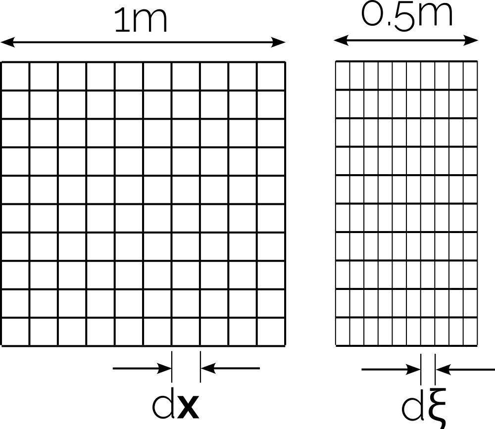
Let's say the left grid is in physical space, that is, the grid in [katex]x[/katex] and [katex]y[/katex] in which we want to obtain our solution, and the grid on the right is the transformed grid in computational space, with [katex]\xi[/katex] and [katex]\eta[/katex] coordinate directions. We can say that going in the physical space from one point to another in the x-direction must be double the distance compared to the same distance travelled in the computational space.
In other words, we can say that if we have [katex]\mathrm{d}x=0.1[/katex], we also have [katex]\mathrm{d}\xi=0.05[/katex]. Logically, this makes sense because we just scaled the domain by a factor of 2 in the x-direction. Since we have not done any changes to this domain in the [katex]y[/katex] direction, we have [katex]\mathrm{d}y=\mathrm{d}\eta[/katex]. But, if we introduced some changes in [katex]y[/katex] as well, or we just rotated the mesh, then our transformation relations would be less obvious, and we will see in a bit how we can compute them without having to think about them too much.
We can rewrite Eq.(47) in matrix form as:
\begin{bmatrix}
\xi_x & \xi_y \\[1em]
\eta_x & \eta_y
\end{bmatrix}
\begin{bmatrix}
\mathrm{d}x \\[1em]
\mathrm{d}y
\end{bmatrix}=
\begin{bmatrix}
\mathrm{d}\xi \\[1em]
\mathrm{d}\eta
\end{bmatrix}
\tag{48}
Eq.(47) shows us how changes in [katex]x[/katex] and [katex]y[/katex] change [katex]\xi[/katex] and [katex]\eta[/katex]. Thus, we can also say that [katex]\xi[/katex] and [katex]\eta[/katex] are functions of [katex]x[/katex] and [katex]y[/katex], and we can express that as:
\xi=f(x,y)\\[1em]
\eta=f(x,y)\tag{49}
Let's turn this around and see what happens if we express [katex]x[/katex] and [katex]y[/katex] as changes in [katex]\xi[/katex] and [katex]\eta[/katex]. Then, we would have the following functional relationship:
x = f(\xi, \eta)\\[1em]
y = f(\xi, \eta)\tag{50}
Using this functional relationship, let's express the total differential for [katex]\xi[/katex] and [katex]\eta[/katex] in Eq.(47) in terms of [katex]x[/katex] and [katex]y[/katex]. This results in:
\mathrm{d}x = \frac{\partial x}{\partial \xi}\mathrm{d}\xi + \frac{\partial x}{\partial \eta}\mathrm{d}\eta = x_\xi\mathrm{d}\xi + x_\eta\mathrm{d}\eta \\[1em]
\mathrm{d}y = \frac{\partial y}{\partial \xi}\mathrm{d}\xi + \frac{\partial y}{\partial \eta}\mathrm{d}\eta = y_\xi\mathrm{d}\xi + y_\eta\mathrm{d}\eta \tag{51}
We may write this again in matrix form as:
\begin{bmatrix}
x_\xi & x_\eta \\[1em]
y_\xi & y_\eta
\end{bmatrix}
\begin{bmatrix}
\mathrm{d}\xi \\[1em]
\mathrm{d}\eta
\end{bmatrix}=
\begin{bmatrix}
\mathrm{d}x \\[1em]
\mathrm{d}y
\end{bmatrix}.
\tag{52}
Our goal now is to write Eq.(48) and Eq.(52) in the same form, i.e. we want to have the vector [katex][\mathrm{d}x, \mathrm{d}y]^T[/katex] on the left-hand side, and the vector [katex][\mathrm{d}\xi, \mathrm{d}\eta]^T[/katex] on the right-hand side. The way to do that is to multiply Eq.(inverse-mapping-matrix-form) by the inverse coefficient matrix. This can be obtained in the following way:
\begin{bmatrix}
x_\xi & x_\eta \\[1em]
y_\xi & y_\eta
\end{bmatrix}^{-1}=
\frac{1}{x_\xi y_\eta - x_\eta y_\xi}
\begin{bmatrix}
y_\eta & -x_\eta \\[1em]
-y_\xi & x_\xi
\end{bmatrix}=
\frac{1}{J}
\begin{bmatrix}
y_\eta & -x_\eta \\[1em]
-y_\xi & x_\xi
\end{bmatrix}
\tag{53}
When we compute the inverse matrix, we need to divide each component by the determinant, i.e. [katex]\det|A|[/katex], where [katex]A[/katex] is the coefficient matrix. We can see that the determinant is:
\det|A| =
\det\Bigg|
\begin{matrix}
x_\xi & x_\eta \\[1em]
y_\xi & y_\eta
\end{matrix}
\Bigg|=
\frac{1}{x_\xi y_\eta - x_\eta y_\xi}=
\frac{1}{J}
\tag{54}
We give the determinant the letter [katex]J[/katex], which stands for the Jacobian. Unfortunately, we also use the term Jacobian for the coefficient matrix containing fluxes when we linearise the Navier-Stokes equation. That process is completely different to the Jacobian we obtain from the coordinate transformation, so I thought I would mention it here in case you google it now, stumble across some other Jacobians, are confused, and subsequently call me a liar. I'm not, CFD is just full of wonderful inconsistencies!
So, let's multiply Eq.(52) by the inverse matrix. Then we get:
\begin{bmatrix}
x_\xi & x_\eta \\[1em]
y_\xi & y_\eta
\end{bmatrix}^{-1}
\begin{bmatrix}
\mathrm{d}x \\[1em]
\mathrm{d}y
\end{bmatrix}=
\begin{bmatrix}
\mathrm{d}\xi \\[1em]
\mathrm{d}\eta
\end{bmatrix}\\[2em]
\frac{1}{J}
\begin{bmatrix}
y_\eta & -x_\eta \\[1em]
-y_\xi & x_\xi
\end{bmatrix}
\begin{bmatrix}
\mathrm{d}x \\[1em]
\mathrm{d}y
\end{bmatrix}=
\begin{bmatrix}
\mathrm{d}\xi \\[1em]
\mathrm{d}\eta
\end{bmatrix}
\tag{55}
Now the left-hand side and right-hand side column vectors are the same as in Eq.(48). Let's compare both equations:
\begin{bmatrix}
\xi_x & \xi_y \\[1em]
\eta_x & \eta_y
\end{bmatrix}
\begin{bmatrix}
\mathrm{d}x \\[1em]
\mathrm{d}y
\end{bmatrix}=
\begin{bmatrix}
\mathrm{d}\xi \\[1em]
\mathrm{d}\eta
\end{bmatrix}
\\[2em]
\frac{1}{J}
\begin{bmatrix}
y_\eta & -x_\eta \\[1em]
-y_\xi & x_\xi
\end{bmatrix}
\begin{bmatrix}
\mathrm{d}x \\[1em]
\mathrm{d}y
\end{bmatrix}=
\begin{bmatrix}
\mathrm{d}\xi \\[1em]
\mathrm{d}\eta
\end{bmatrix}
\tag{56}
Thus, we can see that the following equality must hold by comparison:
\begin{bmatrix}
\xi_x & \xi_y \\[1em]
\eta_x & \eta_y
\end{bmatrix}=
\frac{1}{J}
\begin{bmatrix}
y_\eta & -x_\eta \\[1em]
-y_\xi & x_\xi
\end{bmatrix}\tag{57}
Here, we simply compare the coefficient matrices. They must be equivalent; otherwise, the equality we found for the two equations in Eq.(56) would not hold anymore. This is really useful, because we can now establish a direct mapping from [katex]x,y[/katex] physical space to [katex]\xi,\eta[/katex] computational space, as shown in the following equations:
\xi_x = \frac{1}{J}y_\eta\\[1em]
\xi_y = -\frac{1}{J}x_\eta\\[1em]
\eta_x = -\frac{1}{J}y_\xi\\[1em]
\eta_y = \frac{1}{J}x_\xi
\tag{58}
Return back all the way to our continuity equation example in Eq.(37), we had:
\xi_x\frac{\partial u}{\partial \xi} + \eta_x\frac{\partial u}{\partial \eta} + \xi_y\frac{\partial v}{\partial \xi} + \eta_y\frac{\partial v}{\partial \eta} = 0\tag{59}If you look at the derivatives, we have derivatives of the velocity component [katex]u[/katex] and [katex]v[/katex] with respect to [katex]\xi[/katex] and [katex]\eta[/katex], respectively, but our metrics are evaluated in physical space, i.e. their derivatives are with respect to [katex]x[/katex] and [katex]y[/katex]. But, we just found the relations for expressing metric coefficients in both computational and physical space, i.e. Eq.(58). Using these relations, we can express all derivatives in computational space, i.e. with respect to [katex]\xi[/katex] and [katex]\eta[/katex], and we arrive at:
\frac{1}{J}y_\eta\frac{\partial u}{\partial \xi} - \frac{1}{J}y_\xi\frac{\partial u}{\partial \eta} - \frac{1}{J}x_\eta\frac{\partial v}{\partial \xi} + \frac{1}{J}x_\xi\frac{\partial v}{\partial \eta} = 0
\tag{60}
So, this has all been wonderfully abstract, and if I leave it at this point, I guess you will have more questions than answers. In order to show how we would actually use this in practice, I want to go through a simple example with you. For that, let's look at the following figure, where we have a mesh in physical space on the top, and its transformed mesh in computational space on the bottom:

This grid contains the same number of cells in the x and y directions, and I have also provided the coordinate axes from which we can infer the sizes of different cells. I have also marked two points in physical space, which are labelled as [katex]P_1(x,y)[/katex] and [katex]P_2(x,y)[/katex]. We can find the corresponding points [katex]P_1(\xi,\eta)[/katex] and [katex]P_2(\xi,\eta)[/katex] in computational space.
Our goal now is to evaluate all metric coefficients, that is, those given in Eq.(58). We can use any appropriate gradient approximation method, though I have not seen anyone use anything other than a Taylor-series-based finite difference approximation.
If you go through the above article, or you remember the finite difference approximation by heart, because your supervisor made you, then you may recall that we can approximate a derivative using a second-order central scheme as:
\frac{\partial \phi}{\partial x} \approx \frac{\phi_{i+1,j}-\phi_{i-1,j}}{2\Delta x}\tag{61}We can do exactly the same with the metric coefficients, and simply approximate the relations given in Eq.(58) with second-order central schemes. This is shown below:
x_\xi = \frac{\partial x}{\partial \xi} \approx \frac{x_{i+1,j} - x_{i-1,j}}{2\Delta \xi} \\[1em]
x_\eta = \frac{\partial x}{\partial \eta} \approx \frac{x_{i,j+1} - x_{i,j-1}}{2\Delta \eta} \\[1em]
y_\xi = \frac{\partial y}{\partial \xi} \approx \frac{y_{i+1,j} - y_{i-1,j}}{2\Delta \xi} \\[1em]
y_\eta = \frac{\partial y}{\partial \eta} \approx \frac{y_{i,j+1} - y_{i,j-1}}{2\Delta \eta}\tag{62}
If we want to evaluate these now, we simply check in our figure what the values are. Let's do the first derivative in detail for point [katex]P_1[/katex], and let's say we want to compute [katex]x_\xi[/katex]. From the equation above, we see that to compute [katex]x_\xi[/katex], we need the values for [katex]x_{i+1,j}[/katex], [katex]x_{i-1,j}[/katex], and [katex]\Delta \xi[/katex]. Let's go to our mesh in computational space where [katex]P_1[/katex] is located, that location is denoted now with indices [katex]i,j[/katex].
[katex]P_1[/katex] is located at [katex]x_{i,j}=1[/katex] and [katex]y_{i,j}=1[/katex]. If we now go one cell to the right, we arrive at [katex]i+1,j[/katex], and we can read off the values for [katex]x[/katex] and [katex]y[/katex] again as [katex]x_{i+1,j}=1.5[/katex] and [katex]y_{i+1,j}=1[/katex]. We can do the same by going one cell to the left, and we arrive at [katex]i-1,j[/katex]. Here, we can see that our values for [katex]x[/katex] and [katex]y[/katex] are [katex]x_{i-1,j}=0.5[/katex] and [katex]y_{i-1,j}=1[/katex].
The only remaining value we need is [katex]\Delta \xi[/katex], which we obtain from our computational space. At point [katex]P_1[/katex] in computational space, we see that [katex]\Delta\xi[/katex] is 1. You may ask why, and as we have discussed before, it is up to us, and we can set the spacing however small or large we want. But [katex]\Delta\xi=\Delta\eta=1[/katex] is a common choice.
Now, with these values at hand, let's compute the first metric together:
x_\xi \approx \frac{x_{i+1,j} - x_{i-1,j}}{2\Delta \xi} \approx \frac{1.5 - 0.5}{2 \cdot 1} = 0.5 \\[1em]\tag{63}We simply insert these values and obtain our metric coefficient. For the remaining metrics, we have the following values:
x_\eta \approx \frac{x_{i,j+1} - x_{i,j-1}}{2\Delta \eta} \approx \frac{1 - 1}{2 \cdot 1} = 0 \\[1em]
y_\xi \approx \frac{y_{i+1,j} - y_{i-1,j}}{2\Delta \xi} \approx \frac{1 - 1}{2 \cdot 1} = 0 \\[1em]
y_\eta \approx \frac{y_{i,j+1} - y_{i,j-1}}{2\Delta \eta} \approx \frac{1.25 - 0.75}{2 \cdot 1} = 0.25\tag{64}
To note here is that if we evaluate a derivative in the [katex]\xi[/katex] direction, which corresponds to the [katex]x[/katex] direction in physical space, we change the [katex]i[/katex] index, i.e. we use [katex]i+1[/katex] and [katex]i-1[/katex] to evaluate the derivatives. If the metric coefficient is differentiated with respect to [katex]\eta[/katex], however, which corresponds to the [katex]y[/katex] direction, then we change the [katex]j[/katex] index and get [katex]j+1[/katex] and [katex]j-1[/katex].
The Jacobian [katex]J[/katex] is computed as:
J=\frac{1}{x_\xi y_\eta - x_\eta y_\xi}=\frac{1}{0.5\cdot 0.25 - 0\cdot 0}=\frac{1}{0.125}=8\tag{65}What does this value physically represent? Well, let's go back to our grids and see what grid spacing we have. Selecting any cell that is attached to point [katex]P_1[/katex] (since they all have the same dimensions), we can see that we have [katex]\Delta x=0.5[/katex] and [katex]\Delta y=0.25[/katex]. In computational space, we have [katex]\Delta \xi=\Delta \eta = 1[/katex]. If we compute now the volume (well, area in 2D) of these cells, then we get the following:
- Volume in physical space: [katex]\Delta x\Delta y=0.5\cdot 0.25=0.125[/katex]
- Volume in computational space: [katex]\Delta \xi\Delta \eta = 1\cdot 1=1[/katex]
The ratio of the volumes in physical to computational space is 1:8, and the Jacobian is also [katex]J=8[/katex]. This is the Jacobian here that acts in the same way as the scale in our map example we looked at earlier. It is simply the scale factor between cell volumes. Using these values now, we can insert these into our 2D continuity equation, i.e. Eq.(60), which was given as:
\frac{1}{J}y_\eta\frac{\partial u}{\partial \xi} - \frac{1}{J}y_\xi\frac{\partial u}{\partial \eta} - \frac{1}{J}x_\eta\frac{\partial v}{\partial \xi} + \frac{1}{J}x_\xi\frac{\partial v}{\partial \eta} = 0\tag{66}Now we can discretise this equation at point [katex]P_1[/katex] with the following values:
\frac{1}{8}0.25\frac{\partial u}{\partial \xi} - \frac{1}{8}0\frac{\partial u}{\partial \eta} - \frac{1}{8}0\frac{\partial v}{\partial \xi} + \frac{1}{8}0.5\frac{\partial v}{\partial \eta} = 0 \\[1em]
\frac{1}{32}\frac{\partial u}{\partial \xi} + \frac{1}{16}\frac{\partial v}{\partial \eta} = 0 \\[1em]
\frac{1}{32}\frac{u_{i+1,j}-u_{i-1,j}}{2\Delta\xi} + \frac{1}{16}\frac{v_{i,j+1}-v_{i,j-1}}{2\Delta\eta} = 0 \\[1em]
\frac{u_{i+1,j}-u_{i-1,j}}{64\Delta\xi} + \frac{v_{i,j+1}-v_{i,j-1}}{32\Delta\eta} = 0\tag{67}
Let's initialise our domain with some values and apply some boundary conditions, all in computational space (as we want to evaluate the entire flow in this domain). This is shown in the figure below:

We can see the boundary conditions for [katex]u[/katex] and [katex]v[/katex] everywhere (Dirichlet for the left, top, and bottom face, Neumann for the right face), and inside the domain, all values for [katex]u[/katex] and [katex]v[/katex] are set to zero initially. At location [katex]i,j[/katex], which is at the same location where we evaluated all metric coefficients for point [katex]P_1[/katex], we can write our discretised equation as:
\frac{u_{i+1,j}-u_{i-1,j}}{64\Delta\xi} + \frac{v_{i,j+1}-v_{i,j-1}}{32\Delta\eta} = 0 \\[1em]
\frac{0-1}{64\cdot 1} + \frac{0-0}{32\cdot 1} = 0 \\[1em]
-\frac{1}{64}=0\tag{68}
Clearly, [katex]-(1/64)\ne 0[/katex], so the continuity equation is not satisfied here, and we will have to iterate over this solution and correct it with predictions for the velocity field from the momentum equation. Eventually, the left-hand side will get closer and closer to zero, and we can stop our simulation once the left-hand side is no larger than our convergence criterion, for example, [katex]10^{-8}[/katex]. Then we can say, convergence is achieved if the following holds true:
\nabla\cdot\mathbf{u} \le 10^{-8} \\[1em]
\frac{u_{i+1,j}-u_{i-1,j}}{64\Delta\xi} + \frac{v_{i,j+1}-v_{i,j-1}}{32\Delta\eta} \le 10^{-8} \tag{69}
One thing we should keep in mind is that even though we evaluate all derivatives of [katex]u[/katex] and [katex]v[/katex] in computational space, since we have found the transformation from physical to computational space, the results will be equivalent in physical space. Thus, we can directly map [katex]u[/katex] and [katex]v[/katex] to the physical space and plot our solutions on the arbitrarily shaped geometry there. No need for further transformation.
For completeness, let us look at point [katex]P_2[/katex] as well. The evaluated metric coefficients are given below:
x_\xi \approx \frac{x_{i+1,j} - x_{i-1,j}}{2\Delta \xi} \approx \frac{4 - 3}{2 \cdot 1} = 0.5 \\[1em]
x_\eta \approx \frac{x_{i,j+1} - x_{i,j-1}}{2\Delta \eta} \approx \frac{3.5 - 3.5}{2 \cdot 1} = 0 \\[1em]
y_\xi \approx \frac{y_{i+1,j} - y_{i-1,j}}{2\Delta \xi} \approx \frac{1.5 - 1}{2 \cdot 1} = 0.25 \\[1em]
y_\eta \approx \frac{y_{i,j+1} - y_{i,j-1}}{2\Delta \eta} \approx \frac{1.5 - 1}{2 \cdot 1} = 0.25\tag{70}
The corresponding Jacobian [katex]J[/katex] is evaluated as:
J=\frac{1}{x_\xi y_\eta - x_\eta y_\xi}=\frac{1}{0.5\cdot 0.25 - 0\cdot 0.25}=\frac{1}{0.125}=8\tag{71}So far, we have only evaluated metric coefficients on the internal domain, but once we approach the boundaries, we can no longer use central differencing. Instead, we make use of one-sided approximations to our derivatives, which are shown in the following:
x_\xi \approx \frac{x_{i,j} - x_{i-1,j}}{\Delta \xi} \quad \text{or} \quad x_\xi \approx \frac{x_{i+1,j} - x_{i,j}}{\Delta \xi} \\[1em]
x_\eta \approx \frac{x_{i,j} - x_{i,j-1}}{\Delta \eta} \quad \text{or} \quad x_\eta \approx \frac{x_{i,j+1} - x_{i,j}}{\Delta \eta} \\[1em]
y_\xi \approx \frac{y_{i,j} - y_{i-1,j}}{\Delta \xi} \quad \text{or} \quad y_\xi \approx \frac{y_{i+1,j} - y_{i,j}}{\Delta \xi} \\[1em]
y_\eta \approx \frac{x_{i,j} - x_{i,j-1}}{\Delta \eta} \quad \text{or} \quad y_\eta \approx \frac{y_{i,j+1} - y_{i,j}}{\Delta \eta}\tag{72}
There is one final point. So far, we have only talked about first-order derivatives, i.e. how we transform [katex]\partial/\partial x[/katex], for example, into computational space. However, the Navier-Stokes equations also contain second-order derivatives, such as [katex]\partial^2/\partial x^2[/katex]. How do we deal with these? Well, we simply carry out the transformation twice. Say, for example, we have a Poisson equation of the following form:
\frac{\partial^2}{\partial x^2}\phi + \frac{\partial^2}{\partial y^2}\phi = \frac{\partial}{\partial x}\frac{\partial}{\partial x}\phi + \frac{\partial}{\partial y}\frac{\partial}{\partial y}\phi\tag{73}Then we can insert our transformation relations for [katex]\partial/\partial x[/katex] and [katex]\partial / \partial y[/katex] which results in:
\left(\frac{1}{J}y_\eta\frac{\partial}{\partial \xi} - \frac{1}{J}y_\xi\frac{\partial}{\partial \eta}\right)\left(\frac{1}{J}y_\eta\frac{\partial}{\partial \xi} - \frac{1}{J}y_\xi\frac{\partial}{\partial \eta}\right)\phi + \left(\frac{1}{J}x_\eta\frac{\partial}{\partial \xi} + \frac{1}{J}x_\xi\frac{\partial}{\partial \eta}\right)\left(\frac{1}{J}x_\eta\frac{\partial}{\partial \xi} + \frac{1}{J}x_\xi\frac{\partial}{\partial \eta}\right)\phi = 0 \\[1em]
\tag{74}
Of course, if you feel bored, you can multiply out these parentheses. Most textbooks dealing with coordinate transformation will do that. I won't, because we make our lives harder. First, if we do it by hand, we will probably make a mistake. I have come up with an empirical rule that for each A4 page of derivations I do, there will be at least 1 mistake. Once I implement that into code, nothing will work, even if I have implemented my (wrong) equations correctly.
Sure, we can use tools like SymPy (Python), Matlab, or Maple, and symbolically derive the correct equations (which I tend to do anyway because I know I will make mistakes), but there is another reason. Once we have found the expression for [katex]\partial^2/\partial x^2[/katex], we can implement that, on top of our transformation we already got for [katex]\partial/\partial x[/katex]. More code means more (possible) programming mistakes, more code to test, and more code to maintain.
From a software engineering perspective, we already have a function that can do [katex]\partial/\partial x[/katex]. We can apply it twice to get the second-order derivative. Not only that, perhaps later I want to also introduce solid mechanics, and all of a sudden I have fourth-order derivatives to evaluate. Then we have to find the transformation for [katex]\partial^4/\partial x^4[/katex]; we have to write yet more code and more tests.
Thus, I'd advocate that we leave Eq.(74) as it is, enjoy that we are done with our transformation, and we can extend this easily to arbitrary orders of derivatives if we need to.
Well, at this point, I think we have exhausted our discussion on coordinate transformation. Let's bring all of what we have discussed in the previous section together, specifically, mesh quality metrics and coordinate transformation. Let us now discover how we can automatically create high-quality structured grids without user intervention. They are based on partial differential equations; let's review them next.
Partial Differential Equation-based Structured Mesh Generation
Let's cast our minds back to the early days of CFD. We had a basic understanding of numerical schemes, we knew that the non-linear term is making our life hell, every single day, and we could simulate the Navier-Stokes equations on some very basic grids, similar to the example we looked at in the coordinate transformation section (i.e. channel flows).
It would be an understatement to say that algebraic mesh generators were popular; these were the only mesh generators in use, as the finite difference method was still the default choice in CFD and experimentation with the finite volume and finite element method only started later (when we deal with the finite difference method, we have to use a structured grid).
We discussed briefly how Moore's law tells us that the number of transistors on a chip double every 24 month, at least that was the case up until the mid 2010s, according to MIT. I also mentioned that an ever increasing ceiling for your computational resources mean that you are getting hungry for more.
Sure, back then, you may have been happy with a channel flow geometry in 2D, but then merely 2 years later, you wanted to resolve boundary layers, 2 years later, you wanted turbulence modelling and mesh refinement, and then another 2 years later, you wanted 3D. Soon after that, people started to do DNS simulations of channel flows, some of the most demanding simulations you can think of (still to this day).
Other people enjoyed the abundance of computational power by playing around with new technologies, like the finite volume method and its ability to simulate flows on unstructured grids. Geometries became more complex, first in 2D, but then they quickly transitioned to 3D, and the rest is history. Nowadays, CFD can be used anywhere where there is a flow, but for someone like me (and you?) who was born into the golden age of CFD, it is difficult to appreciate that this was not always the case.
CFD, as a useful tool for research and industrial work, has only really been available for a few decades. There are still industries where CFD could be used, and it would add a lot of value, but it hasn't been picked up by the mainstream yet, and there are, perhaps, only a few people in that area who are playing around with CFD.
With the desire to solve the governing equations of CFD for ever more complex geometries, our mesh generators had to evolve and keep in lockstep with our growing ambitions and capabilities of CFD solvers in those days. Algebraic mesh generators were emerging and becoming more sophisticated, but these required a lot of manual input, and so we wanted automation.
This is when researchers were pondering the following question: "If the governing equation of fluid mechanics is used to advance a simulation in time and space, can a similar set of equations be found that advance a mesh from an initial boundary (the geometry) into the far field?". The search for the perfect equation was one, and people were trying different types of partial differential equations (PDEs).
Let's review a few properties of PDEs that will become important. In general, we can classify a PDE as an elliptic, parabolic, or hyperbolic equation. I have written an entire article about how to classify PDEs, and what these classifications mean (and how we can see that with our own eyes in results and animations). You can find this article here: What are Hyperbolic, parabolic, and elliptic equations in CFD?
In general, to solve a PDE, we need boundary values and/or initial values. These are then classified as boundary value problems (BVP) and initial value problems (IVP). The following holds for elliptic, parabolic, and hyperbolic PDEs:
- Elliptic PDE: Boundary values need to be prescribed (BVP).
- Parabolic PDE: Initial and boundary values need to be prescribed (BVP, IVP).
- Hyperbolic PDE: Initial values need to be prescribed (IVP).
What does that mean in practice? Think of the flow around an airfoil, for example. The boundaries here are the edges around the airfoil, as well as the edges describing the far field of the domain (your inlet, outlet, or far field boundaries). So, if we have a BVP (elliptic, parabolic), we need to specify the point distribution on all boundaries. We also need an initial mesh to begin with.
Hang on! Did I say you need a mesh to generate a mesh with an elliptic equation? And am I not contradicting myself? Isn't an initial mesh the same as an initial value problem? Question upon questions, and if you are wondering, yes, it is probably about this point in which I have a slight regret writing this article. It may have taken you an hour to arrive at this point; I have been writing for 2 months to get here. In any case, let's look at these questions. (I'm kidding, these were some of the best 2 months I spent! No regrets! I <3 CFD ...)
Yes, an elliptic mesh generator may, at first, seem pointless if we have to provide it with an initial mesh, though this statement is the same as saying that CFD solvers are pointless because we have to give them an initial solution. We don't think about the initial solution too much in CFD, and the same is true for elliptic mesh generators. The mesh can be anything; it can have negative volumes, it can have poor quality metrics. Generating a poorly structured mesh automatically isn't complicated.
But is that then not considered an IVP? Well, the way we define an initial condition has to do with marching a mesh in space. So, for example, let's say we use a hyperbolic mesh generator. This is a pure IVP problem. Let's say we want to create a mesh around an airfoil. Then, we specify an initial point distribution around the airfoil, from where we want to march the mesh.
We also have to specify a direction, i.e. do we want to mesh the inside of the airfoil, or do we want to march the mesh into the far field. If we select the far field, then the hyperbolic mesh generator will create cells around the airfoil, layer by layer, in an O-grid type fashion. Notice how we have not specified the location of the far field boundaries; these will be automatically generated as the mesh marches into the far field.
So, an elliptic mesh generator does not advance the solution in space; it merely takes an existing mesh and then solves an elliptic equation on it. What the elliptic PDE does is to update the location of the [katex]x[/katex], [katex]y[/katex], and [katex]z[/katex] coordinates so that, on average, the quality improves. It is common to use a hyperbolic mesh generator first to create a mesh, and then to use an elliptic mesh generator to improve its quality. Though hyperbolic mesh generators are pretty decent when they work, elliptic mesh generators are usually not needed.
Where are parabolic mesh generators? In a nutshell, nowhere. People have fiddled around with them, but they have never made it into the mainstream. The mesh generation techniques you will find in software like Pointwise are based entirely on elliptic and hyperbolic mesh generation. So, let's look at these two different mesh generation approaches in detail and see how we can generate (or improve) a mesh.
Hyperbolic Mesh Generation
Wow, I hope you are all hyped and pumped up just as much as I am. We are going to learn something wonderful in this section. Hyperbolic mesh generators are something truly beautiful, not just in a mathematical sense, but also in a visual sense, i.e. in the grids they can produce. The only slight downside is: it usually doesn't work. Ah well, all of that excitement just went down the gutter ... But let's look at it anyway. If it works, it works really well (and with some tweaking, we can achieve impressive results)!
I mentioned above how we advance the mesh in space in a given direction using a hyperbolic mesh generator, and this is shown below for a cylinder.
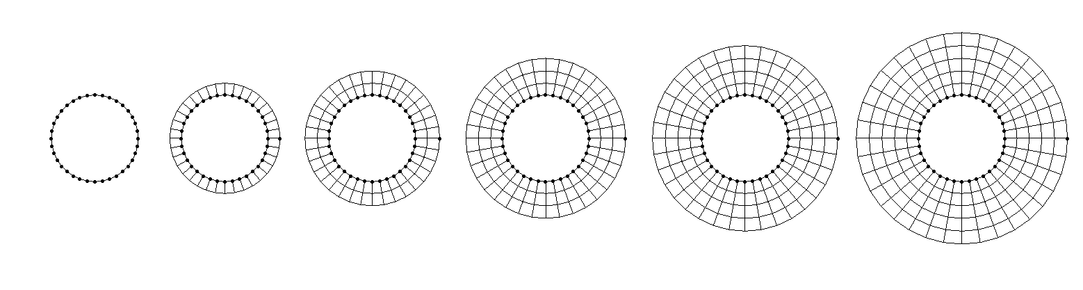
On the left, we specify the initial point distribution on the cylinder, which is our IVP. Then, we solve some hyperbolic equation for each of these points, where we have some update equation of the form:
x^{n+1}_{i,j} = x^{n}_{i,j} + ... \\[1em]
y^{n+1}_{i,j} = y^{n}_{i,j} + ...\tag{75}
Each of these new [katex]x^{n+1}[/katex] and [katex]y^{n+1}[/katex] will give us a new coordinate in space. We connect this new point with the point it originates from, i.e. [katex]x^n[/katex] and [katex]y^n[/katex], as well as adjacent points that we have created, and in this way, we can extrude the mesh into a specified marching direction. In the figure above, we see the initial point distribution on the left, and then 5 iterations of solving a hyperbolic PDE numerically, where each iteration produces a new grid layer around the cylinder.
Which equations should we then use to march the solution through the domain, constructing the computational mesh as we pass through it? We have two unknowns here (the [katex] x [/katex] and [katex] y [/katex] coordinates, and of course a third one, [katex]z[/katex], in 3D space), so we need to solve two partial differential equations. How we obtain these is actually quite ingenious (at least to me, I am easy to impress).
To understand how these equations come about, let's consider the following normal vector in [katex]xy[/katex] space:
n =
\begin{bmatrix}
1\\
1
\end{bmatrix}\tag{76}
This vector simply points at a 45-degree angle to the x- and y-axis. I want to find the vector now that is perpendicular to [katex]n[/katex]. In this simple example, we can say that we simply mirror the vector at either the x or the y-axes, which would give us a perpendicular vector. Let's do that and define both vectors:
n_1^\perp =
\begin{bmatrix}
1\\
-1
\end{bmatrix}\quad
n_2^\perp =
\begin{bmatrix}
-1 \\
1
\end{bmatrix}\quad\tag{77}
Here, [katex]n_1^\perp[/katex] is mirrored along the x-axis and [katex]n_2^\perp[/katex] along the y-axis. There are a few ways how we can check that these vectors are indeed perpendicular to [katex]n[/katex]. You may say, let's use the dot product, and indeed, this can be used. If we find that the dot product is zero for any two given vectors, then we know they are perpendicular. So for the first pairing, we would have:
n\cdot n_1^\perp =
\begin{bmatrix}
1\\
1
\end{bmatrix}\cdot
\begin{bmatrix}
1\\
-1
\end{bmatrix}=
1\cdot 1 + 1\cdot (-1) = 1 - 1 = 0\tag{78}
And for the second pairing, we have:
n\cdot n_2^\perp =
\begin{bmatrix}
1\\
1
\end{bmatrix}\cdot
\begin{bmatrix}
-1\\
1
\end{bmatrix}=
1\cdot (-1) + 1\cdot 1 = -1 + 1 = 0\tag{79}
In both cases, we have confirmed that the dot (or scalar) product is zero, and so the vectors are perpendicular to each other. Job done. But, unfortunately, these relations are not helping us to find a suitable partial differential equation. So, we have to find something else. And this something else starts with the product of the slopes of each vector.
Each vector is essentially just a line. We can find the length of it by taking the magnitude of the vector, and then we can draw a line from the origin to the point specified by the vector itself. So for [katex]n[/katex], we would draw a line from the origin, i.e. [katex]x=0[/katex] and [katex]y=0[/katex] to the points of the vector, i.e. [katex]x=1[/katex] and [katex]y=1[/katex]. The magnitude of [katex]n[/katex] is [katex]\mathrm{mag}(n)=\sqrt{1^2 + 1^2}=\sqrt{2}\approx 1.41[/katex], and indeed, a line from [katex][0,0]^T[/katex] to [katex][1,1]^T[/katex] is exactly [katex]\sqrt{2}[/katex] units long.
The slope of this line can be found by asking, how many units do I have to go up on the y-axis for each unit travelled along the x-axis? In this case, if we go one unit to the right on the x-axis, we go up by one unit, and thus the slope is 1. How can we find that in a mathematical sense? Well, we can use the definition of a slope, which is given as:
m=\frac{y}{x}\tag{80}So, if we plug in values from our vector [katex]n[/katex], then we get:
m_n = \frac{1}{1} = 1\tag{81}We found the same slope. What about our other two vectors [katex]n_1^\perp[/katex] and [katex]n_2^\perp[/katex]? These have the following slopes:
m_{n_1^\perp} = \frac{-1}{1}=-1 \\[1em]
m_{n_2^\perp} = \frac{1}{-1}=-1\tag{82}
What about their products? Let's multiply the slopes by [katex]m_n[/katex]:
m_n \cdot m_{n_1^\perp} = 1 \cdot (-1) = -1 \\[1em]
m_n \cdot m_{n_2^\perp} = 1 \cdot (-1) = -1\tag{83}
In both cases, the product of the slopes is -1. It turns out this is not just the case for this particular vector pairing, but it holds in general. Whenever we have two vectors that are perpendicular, the product of their slopes will always be -1.
We can use this finding now for our quest to find a partial differential equation to create a grid. Think back to our discussion on mesh quality metrics. We said the cells with the least amount of skewness are obtained if our angles within each element are equal to the equilateral angle of that cell type. In 2D, for a quad element (which is the only element we can produce with a structured mesh), the equiangle is 90 degrees.
In other words, the cells with the highest quality (lowest skewness, highest orthogonality) are obtained if we ensure that grid lines that cross are at a 90-degree angle, or perpendicular to each other. Thus, we can locally compute the slope of grid lines, compute their product and enforce that this should be -1. In this way, we naturally inject high-quality cells into our mesh generator, and it will always try to give us cells with the highest quality possible.
So how can we achieve that? We said that the slope can be defined as [katex]m=y/x[/katex]. This is a global view, i.e. I have some [katex]x[/katex] and [katex]y[/katex] values, and I want to find their slope. This works well for lines, but for arbitrary functions, i.e. those with curvature, this approximation may be inaccurate. Instead, we want to check what the slope is at a local point. We can generalise the slope definition then to:
\mathrm{d}m=\frac{\mathrm{d}y}{\mathrm{x}} \\[1em]
\mathrm{y}=m\mathrm{d}x
\tag{84}
This holds for any functional relationship of [katex]y=f(x)[/katex], that is, in this case, [katex]y[/katex] only depends on [katex]x[/katex]. But in our case, we want to create a mesh in 2D space that depends on both [katex]x[/katex] and [katex]y[/katex]. So, what we want is a general functional relationship of the form [katex]g=f(x,y)[/katex]. Using Eq.(\ref{eq:local-slope-definition}), we can extend this equation to make it more general as:
\mathrm{d}g = \frac{\partial g}{\partial x}\mathrm{d}x + \frac{\partial g}{\partial y}\mathrm{d}y\tag{85}Since our derivatives are now depending on two variables, i.e. [katex]x[/katex] and [katex]y[/katex], our ordinary differentials [katex]\mathrm{d}[/katex] have now become partial differentials [katex]\partial[/katex]. If we look at this equation for longer than 2.71 seconds, we may realise that we have already seen this equation before. Yes, it is our good friend, the total differential, from earlier. We were looking at the total differential of [katex]g=\xi[/katex] and [katex]g=\eta[/katex]. As a reminder, these were given as:
\mathrm{d}\xi = \xi_x\partial x + \xi_y\partial y \\[1em]
\mathrm{d}\eta = \eta_x\partial x + \eta_y\partial y
\tag{86}
Here, I have used the shorthand notation again for [katex]\xi_x=\partial \xi / \partial x[/katex]. Let's consider our transformed grid again, which we saw earlier:
If we look at grid lines that go from the bottom to the top, i.e. at [katex]\xi=1,2,3,...,9[/katex], then we can say that along those lines [katex]\mathrm{d}\xi=0[/katex]. The only change along those lines is in the [katex]\eta[/katex] direction. Similarily, we the horizontal grid lines, we can say that [katex]\mathrm{d}\eta=0[/katex] at [katex]\eta=1,2,3[/katex]. With these constraints, we can write Eq.(86) as:
\mathrm{d}\xi = 0 = \xi_x\partial x + \xi_y\partial y \\[1em]
\mathrm{d}\eta = 0 = \eta_x\partial x + \eta_y\partial y\tag{87}
We can rewrite these equations by multiplying the denominators, which results in:
\frac{\partial y}{\partial x}\biggr\rvert_{\xi=\mathrm{const.}} = -\frac{\xi_x}{\xi_y} \\[1em]
\frac{\partial y}{\partial x}\biggr\rvert_{\eta=\mathrm{const.}} = -\frac{\eta_x}{\eta_y}
\tag{88}
Remember, these equations only hold where [katex]\xi=\mathrm{const.}[/katex] and [katex]\eta=\mathrm{const.}[/katex] are imposed as constraints. If this is the case, then we know that multiplying both slopes, i.e. [katex]\partial y/\partial x[/katex] together, must be equal to -1, due to our orthogonality requirement. But let's look at this equation for a second longer, as this really is an important equation.
The left-hand side only contains information about our grid in physical space (i.e. in [katex]x[/katex] and [katex]y[/katex]), while our right-hand side contains information about our computational space (i.e. [katex]\xi[/katex] and [katex]\eta[/katex]). Well, we deal here with partial derivatives with respect to [katex]x[/katex] and [katex]y[/katex], but we have already seen how we can transform those derivatives to be evaluated in computational space, and we will use that transformation again shortly.
But, for now, let us form the product of both equations given in Eq.(88). This results in:
\frac{\mathrm{d}y}{\mathrm{d}x}\biggr\rvert_{\xi=\mathrm{const.}}\cdot\frac{\mathrm{d}y}{\mathrm{d}x}\biggr\rvert_{\eta=\mathrm{const.}} = -1
\tag{89}
Rewriting Eq.(89) using Eq.(88) yields
\left(-\frac{\xi_x}{\xi_y}\right)\cdot\left(-\frac{\eta_x}{\eta_y}\right) = -1.
\tag{90}
Eq.(90) may be reformulated to read
\xi_x\eta_x + \xi_y\eta_y = 0.
\tag{91}
We can now use our mapping from physical to computational space as given by Eq.(58) to transform Eq.(91). To save you some scrolling, Eq.(58) was given as:
\xi_x = \frac{1}{J}y_\eta\\[1em]
\xi_y = -\frac{1}{J}x_\eta\\[1em]
\eta_x = -\frac{1}{J}y_\xi\\[1em]
\eta_y = \frac{1}{J}x_\xi\tag{92}
Using this, Eq.(91) now becomes:
\frac{1}{J}y_\eta\frac{-1}{J}y_\xi + \frac{-1}{J}x_\eta\frac{1}{J}x_\xi = 0 \\[1em]
y_\eta(-y_\xi) + (-x_\eta)x_\xi = 0 \\[1em]
x_\xi x_\eta + y_\xi y_\eta = 0
\tag{93}
This is our first equation. We have two unknowns in this equation, which are [katex]x[/katex] and [katex]y[/katex]. Remember, the partial differentials like [katex]x_\xi[/katex] may be written as [katex]\partial x/\partial \xi[/katex]. When we discretise this metric coefficient, we obtain a term with [katex]\Delta \xi[/katex] and we can set this however small or large we want, thus [katex]\xi[/katex] and [katex]\eta[/katex] are not considered unknowns in Eq.(93).
If we have two unknowns, we need a second equation. Remember, the first equation was constructed to ensure that the orthogonality is maximised (or the skewness is minimised). So, one equation is already responsible for the mesh quality. So for the second equation, we can choose another constraint we want to satisfy. Let's look at the following figure for that:
![A cell being created through a hyperbolic mesh generator. The area of the cell is calculated by [katex] \mathrm{d}c\cdot\mathrm{d}s [/katex] and used in the area approach.](https://raw.githubusercontent.com/cfd-university/articles/refs/heads/main/07_10-key-concepts-everyone-must-understand-in-cfd/assets/12_mesh-generation-in-cfd-all-you-need-to-know-in-one-article/hyperbolic_mesh_area_approach.png)
We have some arbitrarily shaped boundary along which we have an initial set of points, which form the surface mesh. We want to grow layers of cells away from this boundary, and, if this boundary is a solid wall, we typically want to impose some geometric constraints for the cells, typically in the form of a first cell height.
So, we pick a desired [katex]y^+[/katex] value, we compute the first cell height (in meters, which is to be imposed on the mesh), and then we form our surface mesh (initial point distribution on the boundary). Looking at the figure above, this means that we can compute a spacing on the surface mesh based on the point distribution, and with that, we can compute the cell's area (2D) or volume (3D) with the first cell height.
Then, if we also specify a growth rate, we can determine the cell area or volume for subsequent layers as well. Do you know where this is going? When we dealt with the map example, we introduced a scaling factor between our two maps, which turned out to be the Jacobian in our coordinate transformation. Since Eq.(93) is already solved in computational space, we may as well look for an equation in the same space.
The Jacobian was simply the scale between the area or volume in computational space and physical space. And it is exactly this relation which we (ab)use to come up with our second equation. As a reminder, the Jacobian was defined in Eq.(54) as:
J = x_\xi y_\eta - x_\eta y_\xi
\tag{94}
So, using Eq.(93) and Eq.(94), we have two equations for two unknowns. One equation to enforce good orthogonality, and one equation to enforce the first cell height. We provide an initial distribution of points on the surface, and these two equations will then, when solved for [katex]x[/katex] and [katex]y[/katex], determine the coordinates of the vertices one cell layer away from the surface.
These points will then be taken as the new initial data, a new target cell area or volume is computed based on a growth rate, which in turn results in a new Jacobian [katex]J[/katex] in Eq.(94), and the process is repeated. The second evaluation of Eq.(93) and Eq.(94) with new Jacobian and initial point locations will result in the second set of points, forming the second cell layer. The process repeats until all layers have been generated or some other criterion has been reached.
To show this process in action, have a look at the mesh generated around an airfoil. This shows the creation process in the mesh generator Pointwise, which shows each layer as it is being created. Very helpful.
And now, you know the secret behind hyperbolic mesh generators. The final question you may have is, why are these two equations classified as hyperbolic? Well, we could construct a system in which we write our equation in matrix form, and then use the same classification approach we applied for first-order PDEs as discussed in my article on classifying PDEs for fluid dynamics applications. We would get two distinct eigenvalues, and therefore, classify this system as hyperbolic.
Right, now that we can automatically create a grid using hyperbolic mesh generators (or even just using an algebraic approach), it is time for us to look at elliptic mesh generators, which can take our generated mesh and try to improve our quality. Let's look at that next.
Elliptic Mesh Generation
So, we looked at algebraic and hyperbolic mesh generation; the final approach we will look at is elliptical mesh generators. What comes to mind when we talk about elliptic PDEs? Well, if you have studied CFD, or, for that matter, anything related to engineering and applied math, chances are, you have come across the following (generic) equation:
\nabla^2\phi=f
\tag{95}
To many, this will look familiar, and if you have any familiarity with this equation, then you may also know that this equation has a specific name depending on the choice of [katex]f[/katex]. In particular, we have:
- If we set [katex]f=0[/katex], then Eq.(95) is said to be a Laplace equation.
- If we set [katex]f \ne 0[/katex], then Eq.(95) is said to be a Poisson equation.
In incompressible flows, we can't avoid the Poisson equation. If we are dealing with ressure projection methods, such as SIMPLE, PISO, or the Franctional Step Pressure Projection method, Eq.(95) will typically appear in the form of a pressure Poisson equation. We solve it to get an updated pressure field and we use this to correct the velocity field.
If you have dealt with equations before, you may also know that Eq.(95) is the canonical form of an elliptic PDE (or you have astutely read my article on hyperbolic, parabolic, and elliptic equations and how to classify PDEs).
Regardless, the idea behind elliptic mesh generators is to take Eq.(95) and apply it to our mesh. This may appear strange, but let me give you two examples to show you that I have not gone insane and that the solution to Eq.(95) presents indeed a good solution to constructing grids.
First, let's write Eq.(95) in 2D, scalar, form. This results in:
\frac{\partial^2 \phi}{\partial x^2} + \frac{\partial^2 \phi}{\partial y^2}=f(x,y)
\tag{96}
Now I want you to imagine that [katex]\phi=T[/katex], where [katex]T[/katex] represents a temperature. Let's solve Eq.(96) on a square domain with a length of 1 meter on each side. We apply Dirichlet boundary conditions at the top and set [katex]T=1[/katex], i.e. some non-dimensional temperature, and then [katex]T=0[/katex] at the bottom. We'll use Neumann boundary conditions on the left and right sides, meaning that the temperature can develop on these walls according to the surrounding temperature values.
If we solve Eq.(96) now with this set of boundary conditions, then we obtain the temperature distribution as seen in the figure below on the left, which we call solution 1:
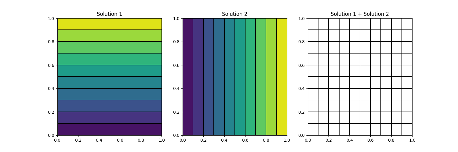
Let us repeat that process, but now rotate the boundary conditions. Now, the right boundary will be of type Dirichlet with a value of [katex]T=1[/katex], and the left boundary will have a value of [katex]T=0[/katex]. The top and bottom boundaries will now be of type Neumann, and the temperature can develop according to its surrounding values again. This is shown in the middle of the figure above and denoted as solution 2.
Eq.(96) is linear, and we are allowed to superimpose solutions. Any superimposed solution is again a valid solution to Eq.(96). So, we can do Solution 1 + Solution 2, and this is shown in the figure above on the right. If you ask me, that looks like a pretty good mesh.
We can repeat the process, but now apply a different set of boundary conditions. For example, in the figure below, I have applied Dirichlet boundary conditions everywhere and have set [katex]T=0[/katex], except on the top and left boundary on the left and middle, respectively, where I have set a value of [katex]T=1[/katex]. I have also superimposed the contour lines again of solutions 1 and 2, which are shown on the right:
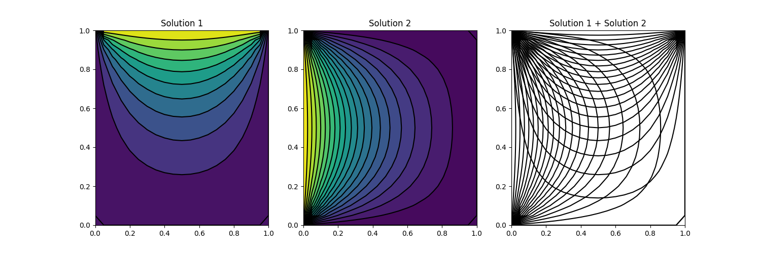
Sure, the corners look a bit strange, but if we just concentrate on the intersections formed in the centre, we see that even for cells that are generated with high curvature, each cell seems to have a good orthogonality and low skewness value. That is, if we look at angles of intersecting grid lines, these tend to be close to 90 degrees.
And this is the secret of elliptic mesh generators: they try to promote cells with good orthogonality, and we will see, in equation form, how they achieve that in just a second.
However, I feel I should stress that the discussion above is just intended to be seen as a motivation. We are not generating contour plots and then taking these to construct our grid. No, I have just shown you what happens when you superimpose two solutions of a Laplace equation, to get a visual intuition for what elliptic grid generators are doing.
So, instead of saying [katex]\phi=T[/katex] in Eq.(95), let us think of a better variable to solve here. Let's stick with a 2D example. It would make sense to say that we have [katex]\phi=x[/katex] and [katex]\phi=y[/katex]. That is, we now have two elliptic equations to solve, and one of them will give us the x coordinates, while the other will provide us with the y coordinates.
However, if we simply used Eq.(95) for [katex]x[/katex] and [katex]y[/katex], then we would have terms like [katex]\partial x/\partial x=1[/katex] and [katex]\partial y/\partial y = 1[/katex]. This would not be very helpful. But, as luck would have it, we just spent an entire section on hyperbolic mesh generators and saw that it is actually quite useful to evaluate our derivatives in computational space, as we can use relations we have already established in the coordinate transformation section.
We will do that in just a second, but first, let's write out Eq.(95) in general, 2D Cartesian form with [katex]f=0[/katex]. This gives us:
\frac{\partial^2 \phi}{\partial x^2} + \frac{\partial^2 \phi}{\partial y^2}=\frac{\partial}{\partial x}\frac{\partial \phi}{\partial x} + \frac{\partial}{\partial y}\frac{\partial \phi}{\partial y} = 0
\tag{97}
We can now use Eq.(40) to express [katex]\partial/\partial x[/katex] and [katex]\partial/\partial y[/katex] in terms of [katex]\xi[/katex] and [katex]\eta[/katex] instead. For this, we ignore any terms that contain either [katex]z[/katex] or [katex]\zeta[/katex] in Eq.(40), as we are now dealing with a 2D case. This results in:
\frac{\partial}{\partial x}\frac{\partial \phi}{\partial x} = \left(\xi_x\frac{\partial}{\partial \xi} + \eta_x\frac{\partial}{\partial \eta}\right)\left(\xi_x\phi_\xi + \eta_x\phi_\eta\right) = 0 \\[1em]
\frac{\partial}{\partial y}\frac{\partial \phi}{\partial y} = \left(\xi_y\frac{\partial}{\partial \xi} + \eta_y\frac{\partial}{\partial \eta}\right)\left(\xi_y\phi_\xi + \eta_y\phi_\eta\right) = 0\tag{98}
Let's carry out the multiplications. This results in:
\frac{\partial}{\partial x}\frac{\partial \phi}{\partial x} = \xi_x\frac{\partial}{\partial \xi}\left(\xi_x\phi_\xi + \eta_x\phi_\eta\right) + \eta_x\frac{\partial}{\partial \eta}\left(\xi_x\phi_\xi + \eta_x\phi_\eta\right) \\[1em]
\frac{\partial}{\partial y}\frac{\partial \phi}{\partial y} = \xi_y\frac{\partial}{\partial \xi}\left(\xi_y\phi_\xi + \eta_y\phi_\eta\right) + \eta_y\frac{\partial}{\partial \eta}\left(\xi_y\phi_\xi + \eta_y\phi_\eta\right)\tag{99}
Let's carry out the differentiation, noting that we have to take the derivative with respect to products, meaning we have to apply the product rule here. This is done as shown below:
\frac{\partial}{\partial x}\frac{\partial \phi}{\partial x} = \xi_x\phi_\xi\frac{\partial}{\partial \xi}(\xi_x) + \xi_x^2\phi_{\xi\xi} + \xi_x\phi_\eta\frac{\partial}{\partial \xi}(\eta_x) + \xi_x\eta_x\phi_{\xi\eta} + \\[1em]
\eta_x\phi_\xi\frac{\partial}{\partial \eta}(\xi_x) + \xi_x\eta_x\phi_{\xi\eta} + \eta_x\phi_\eta\frac{\partial}{\partial \eta}(\eta_x) + \eta_x^2\phi_{\eta\eta} \\[1em]
\frac{\partial}{\partial y}\frac{\partial \phi}{\partial y} = \xi_y\phi_\xi\frac{\partial}{\partial \xi}(\xi_y) + \xi_y^2\phi_{\xi\xi} + \xi_y\phi_\eta\frac{\partial}{\partial \xi}(\eta_y) + \xi_y\eta_y\phi_{\xi\eta} + \\[1em]
\eta_y\phi_\xi\frac{\partial}{\partial \eta}(\xi_y) + \xi_y\eta_y\phi_{\xi\eta} + \eta_y\phi_\eta\frac{\partial}{\partial \eta}(\eta_y) + \eta_y^2\phi_{\eta\eta}\tag{100}
Now we use our transformation relations as seen in Eq.(58) to change the metric coefficients, i.e. [katex]\xi_x[/katex], [katex]\xi_y[/katex], [katex]\eta_x[/katex], and [katex]\eta_y[/katex] to [katex]x_\xi[/katex], [katex]x_\eta[/katex], [katex]y_\xi[/katex], and [katex]y_\eta[/katex], i.e. we change our metric coefficients so they are now evaluated in computational space. This results in:
\frac{\partial}{\partial x}\frac{\partial \phi}{\partial x} = \frac{1}{J}y_\eta\phi_\xi\frac{\partial}{\partial \xi}\left(\frac{1}{J}y_\eta\right) + \frac{1}{J^2}y_\eta^2\phi_{\xi\xi} + \frac{1}{J}y_\eta\phi_\eta\frac{\partial}{\partial \xi}\left(-\frac{1}{J}y_\xi\right) - \frac{1}{J}y_\eta\frac{1}{J}y_\xi\phi_{\xi\eta} - \\[1em]
\frac{1}{J}y_\xi\phi_\xi\frac{\partial}{\partial \eta}\left(\frac{1}{J}y_\eta\right) - \frac{1}{J}y_\eta\frac{1}{J}y_\xi\phi_{\xi\eta} - \frac{1}{J}y_\xi\phi_\eta\frac{\partial}{\partial \eta}\left(-\frac{1}{J}y_\xi\right) - \frac{1}{J^2}y_\xi^2\phi_{\eta\eta} \\[1em]
\frac{\partial}{\partial y}\frac{\partial \phi}{\partial y} = -\frac{1}{J}x_\eta\phi_\xi\frac{\partial}{\partial \xi}\left(-\frac{1}{J}x_\eta\right) - \frac{1}{J^2}x_\eta^2\phi_{\xi\xi} - \frac{1}{J}x_\eta\phi_\eta\frac{\partial}{\partial \xi}\left(\frac{1}{J}x_\xi\right) - \frac{1}{J}x_\eta\frac{1}{J}x_\xi\phi_{\xi\eta} + \\[1em]
\frac{1}{J}x_\xi\phi_\xi\frac{\partial}{\partial \eta}\left(-\frac{1}{J}x_\eta\right) - \frac{1}{J}x_\eta\frac{1}{J}x_\xi\phi_{\xi\eta} + \frac{1}{J}x_\xi\phi_\eta\frac{\partial}{\partial \eta}\left(\frac{1}{J}x_\xi\right) + \frac{1}{J^2}x_\xi^2\phi_{\eta\eta}\tag{101}
Taking the negative sign out of parentheses and writing fractions in a more compact way results in:
\frac{\partial}{\partial x}\frac{\partial \phi}{\partial x} = \phi_\xi\frac{y_\eta}{J}\frac{\partial}{\partial \xi}\left(\frac{y_\eta}{J}\right) + \phi_{\xi\xi}\frac{y_\eta^2}{J^2} - \phi_\eta\frac{y_\eta}{J}\frac{\partial}{\partial \xi}\left(\frac{y_\xi}{J}\right) - \phi_{\xi\eta}\frac{y_\eta y_\xi}{J^2} - \\[1em]
\phi_\xi\frac{y_\xi}{J}\frac{\partial}{\partial \eta}\left(\frac{y_\eta}{J}\right) - \phi_{\xi\eta}\frac{y_\eta y_\xi}{J^2} + \phi_\eta\frac{y_\xi}{J}\frac{\partial}{\partial \eta}\left(\frac{y_\xi}{J}\right) + \phi_{\eta\eta}\frac{y_\xi^2}{J^2} \\[1em]
\frac{\partial}{\partial y}\frac{\partial \phi}{\partial y} = \phi_\xi\frac{x_\eta}{J}\frac{\partial}{\partial \xi}\left(\frac{x_\eta}{J}\right) + \phi_{\xi\xi}\frac{x_\eta^2}{J^2} - \phi_\eta\frac{x_\eta}{J}\frac{\partial}{\partial \xi}\left(\frac{x_\xi}{J}\right) - \phi_{\xi\eta}\frac{x_\eta x_\xi}{J^2} - \\[1em]
\phi_\xi\frac{x_\xi}{J}\frac{\partial}{\partial \eta}\left(\frac{x_\eta}{J}\right) - \phi_{\xi\eta}\frac{x_\eta x_\xi}{J^2} + \phi_\eta\frac{x_\xi}{J}\frac{\partial}{\partial \eta}\left(\frac{x_\xi}{J}\right) + \phi_{\eta\eta}\frac{x_\xi^2}{J^2}\tag{102}
We can now collect terms and factor out the Jacobians. Then, our equations become:
\frac{\partial}{\partial x}\frac{\partial \phi}{\partial x} = \frac{1}{J^2}\left[\phi_{\xi\xi} y_\eta^2 - 2\phi_{\xi\eta}y_\eta y_\xi + \phi_{\eta\eta}y_\xi^2\right] + \\[1em]
\frac{y_\eta}{J}\left[\phi_\xi\frac{\partial}{\partial \xi}\left(\frac{y_\eta}{J}\right) - \phi_\eta\frac{\partial}{\partial \xi}\left(\frac{y_\xi}{J}\right)\right] + \\[1em]
\frac{y_\xi}{J}\left[\phi_\eta\frac{\partial}{\partial \eta}\left(\frac{y_\xi}{J}\right) - \phi_\xi\frac{\partial}{\partial \eta}\left(\frac{y_\eta}{J}\right)\right]  \\[1em]
\frac{\partial}{\partial y}\frac{\partial \phi}{\partial y} = \frac{1}{J^2}\left[\phi_{\xi\xi}x_\eta^2 - 2\phi_{\xi\eta}x_\eta x_\xi + \phi_{\eta\eta}x_\xi^2\right] + \\[1em]
\frac{x_\eta}{J}\left[\phi_\xi\frac{\partial}{\partial \xi}\left(\frac{x_\eta}{J}\right) - \phi_\eta\frac{\partial}{\partial \xi}\left(\frac{x_\xi}{J}\right)\right] + \\[1em]
\frac{x_\xi}{J}\left[\phi_\eta\frac{\partial}{\partial \eta}\left(\frac{x_\xi}{J}\right) - \phi_\xi\frac{\partial}{\partial \eta}\left(\frac{x_\eta}{J}\right)\right]
\tag{103}
At this point, we need to compute the derivatives of the metric coefficients. Remember that the Jacobian was defined in Eq.(54) as:
J=x_\xi y_\eta - x_\eta y_\xi\tag{104}Let us look at the first derivative we have to evaluate in Eq.(103). Inserting the definition for the Jacobian, we get:
\frac{\partial}{\partial \xi}\left(\frac{y_\eta}{x_\xi y_\eta - x_\eta y_\xi}\right)\tag{105}Now we can use the quotient rule to find the derivative. This results in:
\frac{\partial}{\partial \xi}\left(\frac{y_\eta}{x_\xi y_\eta - x_\eta y_\xi}\right) =
\frac{y_{\xi\eta}\left(x_\xi y_\eta - x_\eta y_\xi\right) - y_\eta\left(x_{\xi\xi}y_\eta + x_\xi y_{\xi\eta} - x_{\xi\eta}y_\xi - x_\eta y_{\xi\xi}\right)}{\left(x_\xi y_\eta - x_\eta y_\xi\right)^2} \\[1em]
\frac{\partial}{\partial \xi}\left(\frac{y_\eta}{x_\xi y_\eta - x_\eta y_\xi}\right) =
\frac{Jy_{\xi\eta} - y_\eta\left(x_{\xi\xi}y_\eta + x_\xi y_{\xi\eta} - x_{\xi\eta}y_\xi - x_\eta y_{\xi\xi}\right)}{J^2}
\tag{106}
We can find the derivatives in a similar manner for the remaining metric coefficient derivatives:
\frac{\partial}{\partial \xi}\left(\frac{y_\xi}{x_\xi y_\eta - x_\eta y_\xi}\right) =
\frac{Jy_{\xi\xi} - y_\xi\left(x_{\xi\xi}y_\eta + x_\xi y_{\xi\eta} - x_{\xi\eta}y_\xi - x_\eta y_{\xi\xi}\right)}{J^2}\tag{107}
\frac{\partial}{\partial \eta}\left(\frac{y_\eta}{x_\xi y_\eta - x_\eta y_\xi}\right) =
\frac{Jy_{\eta\eta} - y_\eta\left(x_{\xi\eta}y_\eta + x_\xi y_{\eta\eta} - x_{\eta\eta}y_\xi - x_\eta y_{\xi\eta}\right)}{J^2}\tag{108}
\frac{\partial}{\partial \eta}\left(\frac{y_\xi}{x_\xi y_\eta - x_\eta y_\xi}\right) =
\frac{Jy_{\xi\eta} - y_\xi\left(x_{\xi\eta}y_\eta + x_\xi y_{\eta\eta} - x_{\eta\eta}y_\xi - x_\eta y_{\xi\eta}\right)}{J^2}
\tag{109}
We also have derivatives of [katex]x_\xi[/katex] and [katex]x_\eta[/katex] with respect to [katex]\xi[/katex] and [katex]\eta[/katex] in Eq.(103), i.e. for the second-order derivative of [katex]\phi[/katex] in the y-direction. Let us determine these in a similar way:
\frac{\partial}{\partial \xi}\left(\frac{x_\eta}{x_\xi y_\eta - x_\eta y_\xi}\right) =
\frac{Jx_{\xi\eta} - x_\eta\left(x_{\xi\xi}y_\eta + x_\xi y_{\xi\eta} - x_{\xi\eta}y_\xi - x_\eta y_{\xi\xi}\right)}{J^2}\tag{110}
\frac{\partial}{\partial \xi}\left(\frac{x_\xi}{x_\xi y_\eta - x_\eta y_\xi}\right) =
\frac{Jx_{\xi\xi} - x_\xi\left(x_{\xi\xi}y_\eta + x_\xi y_{\xi\eta} - x_{\xi\eta}y_\xi - x_\eta y_{\xi\xi}\right)}{J^2}\tag{111}
\frac{\partial}{\partial \eta}\left(\frac{x_\eta}{x_\xi y_\eta - x_\eta y_\xi}\right) =
\frac{Jx_{\eta\eta} - x_\eta\left(x_{\xi\eta}y_\eta + x_\xi y_{\eta\eta} - x_{\eta\eta}y_\xi - x_\eta y_{\xi\eta}\right)}{J^2}\tag{112}
\frac{\partial}{\partial \eta}\left(\frac{x_\xi}{x_\xi y_\eta - x_\eta y_\xi}\right) =
\frac{Jx_{\xi\eta} - x_\xi\left(x_{\xi\eta}y_\eta + x_\xi y_{\eta\eta} - x_{\eta\eta}y_\xi - x_\eta y_{\xi\eta}\right)}{J^2}
\tag{113}
We can now plug Eq.(106) to Eq.(113) into Eq.(103) to resolve all derivatives. This results in:
\frac{\partial}{\partial x}\frac{\partial \phi}{\partial x} = \frac{1}{J^2}\left[\phi_{\xi\xi} y_\eta^2 - 2\phi_{\xi\eta}y_\eta y_\xi + \phi_{\eta\eta}y_\xi^2\right] + \\[1em]
\frac{y_\eta}{J}\left[\phi_\xi\frac{Jy_{\xi\eta} - y_\eta\left(x_{\xi\xi}y_\eta + x_\xi y_{\xi\eta} - x_{\xi\eta}y_\xi - x_\eta y_{\xi\xi}\right)}{J^2} - \phi_\eta\frac{Jy_{\xi\xi} - y_\xi\left(x_{\xi\xi}y_\eta + x_\xi y_{\xi\eta} - x_{\xi\eta}y_\xi - x_\eta y_{\xi\xi}\right)}{J^2}\right] + \\[1em]
\frac{y_\xi}{J}\left[\phi_\eta\frac{Jy_{\xi\eta} - y_\xi\left(x_{\xi\eta}y_\eta + x_\xi y_{\eta\eta} - x_{\eta\eta}y_\xi - x_\eta y_{\xi\eta}\right)}{J^2} - \phi_\xi\frac{Jy_{\eta\eta} - y_\eta\left(x_{\xi\eta}y_\eta + x_\xi y_{\eta\eta} - x_{\eta\eta}y_\xi - x_\eta y_{\xi\eta}\right)}{J^2}\right]  \\[1em]
\frac{\partial}{\partial y}\frac{\partial \phi}{\partial y} = \frac{1}{J^2}\left[\phi_{\xi\xi}x_\eta^2 - 2\phi_{\xi\eta}x_\eta x_\xi + \phi_{\eta\eta}x_\xi^2\right] + \\[1em]
\frac{x_\eta}{J}\left[\phi_\xi\frac{Jx_{\xi\eta} - x_\eta\left(x_{\xi\xi}y_\eta + x_\xi y_{\xi\eta} - x_{\xi\eta}y_\xi - x_\eta y_{\xi\xi}\right)}{J^2} - \phi_\eta\frac{Jx_{\xi\xi} - x_\xi\left(x_{\xi\xi}y_\eta + x_\xi y_{\xi\eta} - x_{\xi\eta}y_\xi - x_\eta y_{\xi\xi}\right)}{J^2}\right] + \\[1em]
\frac{x_\xi}{J}\left[\phi_\eta\frac{Jx_{\xi\eta} - x_\xi\left(x_{\xi\eta}y_\eta + x_\xi y_{\eta\eta} - x_{\eta\eta}y_\xi - x_\eta y_{\xi\eta}\right)}{J^2} - \phi_\xi\frac{Jx_{\eta\eta} - x_\eta\left(x_{\xi\eta}y_\eta + x_\xi y_{\eta\eta} - x_{\eta\eta}y_\xi - x_\eta y_{\xi\eta}\right)}{J^2}\right]
\tag{114}
Now we can define the following variables:
S_{y_\eta} = \frac{y_\eta}{J}\left[\phi_\xi\frac{Jy_{\xi\eta} - y_\eta\left(x_{\xi\xi}y_\eta + x_\xi y_{\xi\eta} - x_{\xi\eta}y_\xi - x_\eta y_{\xi\xi}\right)}{J^2} - \phi_\eta\frac{Jy_{\xi\xi} - y_\xi\left(x_{\xi\xi}y_\eta + x_\xi y_{\xi\eta} - x_{\xi\eta}y_\xi - x_\eta y_{\xi\xi}\right)}{J^2}\right]
\tag{115}
S_{y_\xi} = \frac{y_\xi}{J}\left[\phi_\eta\frac{Jy_{\xi\eta} - y_\xi\left(x_{\xi\eta}y_\eta + x_\xi y_{\eta\eta} - x_{\eta\eta}y_\xi - x_\eta y_{\xi\eta}\right)}{J^2} - \phi_\xi\frac{Jy_{\eta\eta} - y_\eta\left(x_{\xi\eta}y_\eta + x_\xi y_{\eta\eta} - x_{\eta\eta}y_\xi - x_\eta y_{\xi\eta}\right)}{J^2}\right]\tag{116}
S_{x_\eta} = \frac{x_\eta}{J}\left[\phi_\xi\frac{Jx_{\xi\eta} - x_\eta\left(x_{\xi\xi}y_\eta + x_\xi y_{\xi\eta} - x_{\xi\eta}y_\xi - x_\eta y_{\xi\xi}\right)}{J^2} - \phi_\eta\frac{Jx_{\xi\xi} - x_\xi\left(x_{\xi\xi}y_\eta + x_\xi y_{\xi\eta} - x_{\xi\eta}y_\xi - x_\eta y_{\xi\xi}\right)}{J^2}\right]\tag{117}
S_{x_\xi} = \frac{x_\xi}{J}\left[\phi_\eta\frac{Jx_{\xi\eta} - x_\xi\left(x_{\xi\eta}y_\eta + x_\xi y_{\eta\eta} - x_{\eta\eta}y_\xi - x_\eta y_{\xi\eta}\right)}{J^2} - \phi_\xi\frac{Jx_{\eta\eta} - x_\eta\left(x_{\xi\eta}y_\eta + x_\xi y_{\eta\eta} - x_{\eta\eta}y_\xi - x_\eta y_{\xi\eta}\right)}{J^2}\right]
\tag{118}
With these source terms defined, we can insert Eq.(115) to Eq.(118) into Eq.(114) and get:
\frac{\partial}{\partial x}\frac{\partial \phi}{\partial x} = \frac{1}{J^2}\left[\phi_{\xi\xi} y_\eta^2 - 2\phi_{\xi\eta}y_\eta y_\xi + \phi_{\eta\eta}y_\xi^2\right] + S_{y_\eta} + S_{y_\xi} \\[1em]
\frac{\partial}{\partial y}\frac{\partial \phi}{\partial y} = \frac{1}{J^2}\left[\phi_{\xi\xi}x_\eta^2 - 2\phi_{\xi\eta}x_\eta x_\xi + \phi_{\eta\eta}x_\xi^2\right] + S_{x_\eta} + S_{x_\xi}
\tag{119}
Looking back at Eq.(97), we had:
\frac{\partial^2 \phi}{\partial x^2} + \frac{\partial^2 \phi}{\partial y^2}=\frac{\partial}{\partial x}\frac{\partial \phi}{\partial x} + \frac{\partial}{\partial y}\frac{\partial \phi}{\partial y} = 0\tag{120}We can now insert here our definition that we obtained from Eq.(119) and obtain:
\frac{1}{J^2}\left[\phi_{\xi\xi} y_\eta^2 - 2\phi_{\xi\eta}y_\eta y_\xi + \phi_{\eta\eta}y_\xi^2\right] + S_{y_\eta} + S_{y_\xi} + \\[1em]
\frac{1}{J^2}\left[\phi_{\xi\xi}x_\eta^2 - 2\phi_{\xi\eta}x_\eta x_\xi + \phi_{\eta\eta}x_\xi^2\right] + S_{x_\eta} + S_{x_\xi} = 0\tag{121}
Let's define [katex]S = S_{y_\eta} + S_{y_\xi} + S_{x_\eta} + S_{x_\xi}[/katex], and multiply by [katex]J^2[/katex], then we have:
\left[\phi_{\xi\xi} y_\eta^2 - 2\phi_{\xi\eta}y_\eta y_\xi + \phi_{\eta\eta}y_\xi^2\right] + \\[1em]
\left[\phi_{\xi\xi}x_\eta^2 - 2\phi_{\xi\eta}x_\eta x_\xi + \phi_{\eta\eta}x_\xi^2\right] + S\cdot J^2 = 0\tag{122}
Now we collect terms and group them together based on [katex]\phi[/katex]. This results in:
\phi_{\xi\xi}(y_\eta^2 + x_\eta^2) - 2\phi_{\xi\eta}(x_\xi x_\eta + y_\xi y_\eta) + \phi_{\eta\eta}(y_\xi^2 + x_\xi^2) + S\cdot J^2 = 0\tag{123}And now, why not, let us also introduce the following shorthand notations:
a = y_\eta^2 + x_\eta^2\\[1em]
b = x_\xi x_\eta + y_\xi y_\eta \\[1em]
c = y_\xi^2 + x_\xi^2 \\[1em]
d = S\cdot J^2
\tag{124}
Then, we obtain the following equation:
\phi_{\xi\xi}a - 2\phi_{\xi\eta}b + \phi_{\eta\eta}c + d = 0\tag{125}And this is our final equation for the elliptic mesh generator. We can now insert [katex]x[/katex] and [katex]y[/katex] for [katex]\phi[/katex] and obtain the following equations for our mesh generator:
x_{\xi\xi}a - 2x_{\xi\eta}b + x_{\eta\eta}c + d = 0 \\[1em]
y_{\xi\xi}a - 2y_{\xi\eta}b + y_{\eta\eta}c + d = 0
\tag{126}
Now, there is a reason why I went through the derivation in depth, because there is one aspect I want you to take away from this. Have a look at Eq.(124) for a moment. We sort of saw this already before, didn't we? In Eq.(93), we derived the orthogonality constraint for the hyperbolic mesh generator. The equation was:
x_\xi x_\eta + y_\xi y_\eta = 0\tag{127}Compare that to the [katex]b[/katex] coefficient in Eq.(124) and we'll notice that these are the same. Thus, the transformed second-order partial differential equation contains a term that also imposes an orthogonality constraint. This means elliptic mesh generators will also maximise the orthogonality in our mesh for free.
So, how would that look? Remember our airfoil example that we looked at in the hyperbolic mesh generator section? I showed you how we could generate a mesh using the hyperbolic mesh generator and how it will generate the mesh layer by layer. Let's take this mesh and put it through our elliptic mesh generator and see what the final mesh will look like:
What do we think? Is it good? Is it bad? Well, certainly it has improved the mesh in the far field, but near the trailing edge of the airfoil, we certainly have some problematic cells. In reality, we will need to impose some constraints, for example, to reduce the strength of the mesh generator near solid boundaries.
There is one final aspect I want to discuss around elliptic mesh generators, I promise, we'll look at something else afterwards. I want to leave you with an intuitive understanding of elliptic equations and why they are useful in the context of mesh generation. For this, let us consider, again, the 2D Laplace equation in Cartesian, scalar form, which is given as:
\frac{\partial^2\phi}{\partial x^2} + \frac{\partial^2\phi}{\partial y^2} = 0\tag{128}Let us quickly discretise it using the finite difference method. If you want to see how I get to the following equation, have a look at my derivation in my article on numerical discretisation procedures. Using a second-order central scheme, we obtain the following equation:
\frac{\phi_{i+1,j}-2\phi_{i,j}+\phi_{i-1,j}}{2\Delta x} + \frac{\phi_{i,j+1}-2\phi_{i,j}+\phi_{i,j-1}}{2\Delta y} = 0\tag{129}Let's make the assumption that [katex]\Delta x = \Delta y[/katex]. We call the new spacing [katex]\Delta s[/katex], i.e. we have [katex]\Delta s = \Delta x = \Delta y[/katex]. I am also going to use a different type of indices. Let's use the following description for index pairs:
i,j = \text{central} \\
i+1,j = \text{right} \\
i-1,j = \text{left} \\
i,j+1 = \text{top} \\
i,j-1 = \text{bottom}\tag{130}
This helps us simplify the equation above to:
\frac{\phi_\text{left} + \phi_\text{right} + \phi_\text{top} + \phi_\text{bottom} - 4\phi_\text{central}}{2\Delta s} = 0\tag{131}Let's make one further simplification and say that [katex]\phi_\text{left} = \phi_\text{right} = \phi_\text{top} = \phi_\text{bottom}[/katex]. If this is the case, then we can replace these terms with, say [katex]4\phi_\text{left}[/katex] (or any other location). Then, we get:
\frac{4\phi_\text{left} - 4\phi_\text{central}}{2\Delta s} = 0\tag{132}Under which condition is this equation satisfied, i.e. equal to zero? When [katex]\phi_\text{left} = \phi_\text{dentral}[/katex], or, [katex]\phi_\text{central} = \phi_\text{left} = \phi_\text{right} = \phi_\text{top} = \phi_\text{bottom}[/katex]
Elliptic equations always seek to locally average the quantity they are solving for (in this case, [katex]\phi[/katex]), so that any gradients vanish. The diffusion operator in the Navier-Stokes equation is elliptic in nature, and using my favourite example of a tea bag being placed in a cup of hot water, we initially have a high tea concentration in the tea bag but no tea inside the hot water.
The diffusion operator will diffuse tea out of the tea bag, and over time, we will have the same tea concentration everywhere in the hot water. If we were to measure the tea concentration gradient anywhere in the water, we would find that it is zero (in other words, the tea is equally distributed and we don't have pockets of hot water in which there is no tea, while in other areas there is a strong concentration of tea).
Bringing this back to our elliptic mesh generator, the elliptic nature helps us to redistribute the points in space. Our Eqs.(126) will take the initial distribution of points in space and then move them so that the average distance between the points equalises. Combine this with the orthogonality constraint that is naturally baked into the solution, and you have a pretty powerful mesh generation tool.
OK, enough of structured mesh generation, let us now go to the next section and see how we can deal with unstructured grids.
Unstructured mesh generation
You might think unstructured mesh generation must be more complicated than structured mesh generation. Well, discretising unstructured grids will take some more effort, as we now have to include geometric considerations, and we have to think about things like non-orthogonal corrections for diffusive operators, but unstructured mesh generation is really rather straightforward.
In this section, you won't find many equations or lengthy derivations, though that doesn't mean that you can make this topic arbitrarily complex. But, if we want to build up an understanding of what different algorithms are, how they work, and how we may implement that into code, we don't need that much math, and, hopefully, this means I won't spend another month writing about unstructured grids.
I don't personally mind, but the longer it takes me to get these articles out, the more emails I have to respond to confirming that I have not given up on this website, or that I am, indeed, still alive.
So, in this section, I want to look at the two most common unstructured meshing algorithms that are used to connect vertices in a way that maximises quality. These algorithms are:
- The Delaunay algorithm
- The advancing front algorithm
None of these two approaches will actually generate points/vertices; they simply take some randomly seeded points within the domain and connect them with triangles. The point/vertex generation is part of another process called the domain nodalisation, which places points everywhere in the domain. These points/vertices are then used by either the Delaunay or the advancing front algorithm to generate the unstructured mesh.
Before we can do that, though, I want to return to the unstructured data structure and spend some time exploring how we store unstructured grids. Once you know that, it will be easy to understand any unstructured grid format. We looked at that briefly before when we contrasted structured with unstructured grids, though I used most of that time shaming my former flatmates. Also, I looked at that as well when discussing unstructured mesh reading with the CGNS data format.
So, we will quickly review the data structure of unstructured grids, and then look at domain nodalisation, as well as the Delaunay and the advancing front method.
Data Structure Requirements for Unstructured Grids
Let's look at an example grid with two different cell types and see how we would store the unstructured grid data for these grids. An example of two grids using quad and triangle cells is shown below.

Each vertex has a number to uniquely identify it, and each cell has its own letter for the same purpose. If we want to work with this grid, or simply just store it, then we need to think about what information we need to store and in which way. The first thing we may want to store is the cells, and which vertices are used to create a given cell. This is shown in the table below for the quad mesh shown on the left in the figure above.
| Cell ID | Vertex 1 | Vertex 2 | Vertex 3 | Vertex 4 |
|---|---|---|---|---|
| A | 0 | 1 | 4 | 3 |
| B | 1 | 2 | 5 | 4 |
| C | 3 | 4 | 7 | 6 |
| D | 4 | 5 | 8 | 7 |
Equally, we can find the cell information for the triangle mesh shown above on the right. This is given in the table below.
| Cell ID | Vertex 1 | Vertex 2 | Vertex 3 |
|---|---|---|---|
| A | 0 | 4 | 3 |
| B | 0 | 1 | 4 |
| C | 1 | 5 | 4 |
| D | 1 | 2 | 5 |
| E | 3 | 7 | 6 |
| F | 3 | 4 | 7 |
| G | 4 | 8 | 7 |
| H | 4 | 5 | 8 |
We see that we need to store 4 vertices per cell in the first case, while we store only 3 vertices in the second case. If we think about it, the number of vertices for each standard element type in 2D is:
- triangle: 3 vertices
- quad: 4 vertices
In 3D, we have the following number of vertices:
- tetra: 4 vertices
- pyramid: 5 vertices
- prism: 6 vertices
- hexa: 8 vertices
As long as we know the dimension (2D or 3D, let's be honest, if we run a 1D case, we won't use an unstructured mesh for this ...), we can infer the element type from the number of vertices, as this number is unique. This approach breaks down, of course, once we start to use polygons and polyhedra.
Once we have the so-called connectivity table, sometimes also called the lookup table, i.e. the vertices that belong to each cell, we also need to store the coordinates of each vertex. If we assume that vertex 0, as shown in the figure above, is located at [katex]x=0[/katex], [katex]y=0[/katex], and that vertex 8 is located at [katex]x=1[/katex], [katex]y=1[/katex], then we can find the coordinates for each vertex. Both the grids shown on the left and right in the figure above will have the following coordinates for their vertices:
| Vertex ID | [katex]x[/katex] coordinate | [katex]y[/katex] coordinate |
|---|---|---|
| 0 | 0.0 | 0.0 |
| 1 | 0.5 | 0.0 |
| 2 | 1.0 | 0.0 |
| 3 | 0.0 | 0.5 |
| 4 | 0.5 | 0.5 |
| 5 | 1.0 | 0.5 |
| 6 | 0.0 | 1.0 |
| 7 | 0.5 | 1.0 |
| 8 | 1.0 | 1.0 |
Now we have specified almost everything. With the coordinates of the vertices and the vertex IDs that make up individual cells, we can already do quite a lot. For example, we can compute each cell's area, we can compute the cell's centroid and then the orthogonality, skewness, aspect ratio, and area change. But one crucial aspect is missing, and that is the boundary condition information.
We need to know which edges on the boundaries should be grouped together. We can then assign a specific boundary condition here, for example, a wall, or a velocity inlet, and then the solver will know what conditions to impose here. For example, if we group the two edges at the top of the domain together, we could set these as a wall boundary condition. Then, our solver can specify that the velocity is zero at the face centroid, and the pressure is a Neumann-type condition, and so copied from the closest centroid.
In our example, let's say that each side should be grouped into its own boundary patch, so that we have an east, west, north, and south boundary patch. Then, the edges need to be mapped together as shown in the following table:
| Boundary ID | edges |
|---|---|
| south | {(0, 1), (1, 2)} |
| east | {(2, 5), (5, 8)} |
| north | {(8, 7), (7, 6)} |
| west | {(6, 3), (3, 0)} |
If you now inspect any mesh file format that stores unstructured grids (and one that you can actually look at, i.e. one that is written in ASCII), you will find these three tables everywhere. You always get your cell connectivity table, your coordinates of vertices, and the boundary patch information. If you don't, you'll miss something.
I should also stress here that this is the absolute minimum we need, but we can store more if we want. For example, in the finite volume method, we are working with a face-based approach, meaning that we typically interpolate values from cell centroids to face centres (using an upwind scheme, for example). This means that, for each cell, we need to know its neighbouring cells.
We can always compute that. The trick is to first identify how many vertices we need to define our faces. In our example, we are currently dealing with a 2D grid, so faces will consist of 1D edges and will only have 2 vertices. Thus, any two cells that have 2 vertices in common must share a face. Let's look at our cells again, which I showed above:
For cell A on the left, we can see that it shares vertices 1 and 4 with cell B, and therefore, they must be neighbours. Similarly, vertices 3 and 4 are shared with cell C, and so A and C must also be neighbours. In 3D, we may have triangles or quads as faces, and so need to check for 3 or 4 vertices that are in common for each element.
If we implemented this into code, we may create a loop which first loops over all cells, and then a second loop that loops over all cells except the cell we are at, to check if any of these cell pairs share the required number of vertices. If that is the case, we have found our neighbour. The problem with this naive implementation is that we have a loop within a loop, which we should avoid at all costs.
The reason is that this is very costly. Imagine you have 1 million cells, and for each cell, you have to check against all 999,999 other cells if they are neighbours of your current element. You have to do this check 1 million times. I have implemented this to see how slow it is, and after about 10,000 elements, I gave up. Any more than that and you start to wait tens of seconds or minutes. And, the wait time increases exponentially.
There are better ways to implement this, and the gold standard is described by Lohner in Section 2.2 of his book Applied Computational Fluid Dynamics Techniques: An Introduction Based on Finite Element Methods. Probably worth its own article at some point ...
However, while we generate a mesh, we typically have that information available, or at least can store it very easily during the mesh generation process, and so some mesh file formats will also give you this information for free. The OpenFOAM mesh file format, for example, provides a file called neighbour, where this information is provided (in the form of a pair, where two subsequent numbers indicate two cell IDs that share a face).
Thus, if you are starting out writing your own solver, using a file format like this can actually save you a lot of headaches, as writing the algorithm to find cells that share a face can be difficult, especially if it should be efficient and fast.
OK, enough, I hear you scream, when are we getting to the juicy part? OK, OK, let's move on. Next up: Domain nodalisation.
Domain nodalisation
Domain nodalisation really is the heart of unstructured mesh generation. Get this part right, and it doesn't really matter what approach we later take; any approach will likely lead to a good, high-quality, unstructured grid. The question then becomes, how should we insert these points? There are a few possibilities; let us look at a selection of approaches that were used historically, right through to what is in use today.
Random points
The simplest approach we can think of is one where we insert points at random. As is so often the case in CFD, the simplest approach is rarely the best. Let's see why. In the figure shown below, we have a square domain with a cylinder on the inside. We want to generate a mesh so that the cylinder on the inside is connected to the boundaries in the far field.

If we choose to randomly insert points, as is shown in the middle, then we have no control over the placement of the points. Some may be located inside the cylinder or outside of the domain, though this is something we can easily fix with some additional code (e.g. deleting out-of-bound points). However, if we wanted to have some locally refined grid around the cylinder, or in the wake, or for that matter, anywhere, we have absolutely no control over point placements.
The other problem is shown on the right of the figure, where the points have been connected to form a triangular mesh. Just looking at the area change and skewness, we can see that this mesh is not really of high quality. So, not only does this mesh not capture any of the flow features we want (boundary layers, wakes), but what little it does capture will be influenced by the poor grid quality, possibly even leading to divergence.
Random points used as a domain nodalisation technique are a thought experiment to get thinking about how to best insert points, but they are not to be used in an actual mesh generator. What else could we use?
Using a structured background grid
Well, how about we just use a structured grid? We could just place a structured grid through our domain, remove any points that are out of bounds (e.g. inside our cylinder), and then snap points close to the cylinder onto its surface. We can then turn all of our structured quad elements into triangles (2D) or hexa elements into 6 pyramids (3D). Anyone who has ever dealt with pyramids will now want to shoot me for the last sentence ...
In any case, this is a viable approach, and it is schematically shown in the figure below:

Well, if we were to follow this approach, then we wouldn't really gain anything over a structured grid, apart from making adaptive mesh refinement a lot easier (since we converted from structured quad cells to unstructured triangles, which gives us greater geometric flexibility). Otherwise, we may just use a structured grid, have a simpler discretisation, and not bother with the additional complexity of having to deal with an unstructured grid's data structure.
Using an N-tree background grid
Extending the idea of a structured grid, we could use an N-tree grid, where the N refers to the tree used for a given dimension. In 1D, we deal with a binary tree, in 2D, we deal with a quadtree, and in 3D, we deal with an octree. N-trees allow for non-conformal mesh refinement, having hanging nodes. These allow for structured-like grids to have local mesh refinement, as shown in the figure below (see second domain from the left):

N-tree-based approaches are very popular in mesh generation these days, and you will find most mesh generators use this approach (ANSYS Fluent meshing, OpenFOAM's snappyHexMesh, Star-CCM+, Converge CFD, Numeca (wild guess), and probably more that I am not aware of ...). The main idea is that we gain the ease of using a structured grid for most of the domain, but then also gain the flexibility of locally refining our mesh in regions where we need to have additional resolution, e.g. near solid walls and in wakes.
In fact, N-tree-based approaches are so popular that most solvers will simply take the generated mesh from the N-tree and use that for its simulation (usually coupled with some additional inflation layer growth mechanism to capture turbulent boundary layers).
If we don't have any inflation layers, though, we can easily place a so-called space-filling curve through our N-tree, which can be used to decompose our domain into M different subdomains, which can then be solved by M different processors to speed up the simulation. Domain decomposition is a topic in its own right and can get difficult for complex (unstructured) domains. Space-filling curves make this very easy, and thus N-trees become a lucrative choice for complex problems.
Using a size field function
Another popular approach is that of using a size field function. The way it works is rather different from any of the previous approaches (though it could be understood to be a random point insertion algorithm with some constraints applied to it). Let's assume we want to mesh a square domain again, and we have the points on each side given, so we know the spacing on each boundary.
A size field function [katex]h = f(x,y)[/katex] would give us the size, or length, of a triangle edge at any given point in [katex]x[/katex] and [katex]y[/katex]. Thus, if I want to construct a triangle at, say, [katex]x=0.457[/katex] and [katex]y=0.12[/katex], and I know that [katex]h(0.457, 0.12) = 0.054[/katex], then my mesh algorithm will generate a triangle (or quad) where each edge is about 0.054 meters long.
Well, approximately, it is an over-constrained problem. The triangle (or quad) to the right may have a size field value of [katex]h=0.07[/katex]. But, since one edge is shared between both triangles (or quads), which have different-sized field values, we can only find a compromise here (for example, the average of the two).
How could we find such a size field function? If we know the geometry analytically, then we could come up with an algebraic equation and tweak the size field to our liking, but that is not a general approach and is limited to that geometry only. So, this isn't a great approach.
A more common approach is to use a PDE and evolve that in space to find a size field function numerically. To do that, ironically, we need to have a mesh in the first place to solve this PDE on. However, as we will see in a second, it doesn't really matter what mesh we use, and so perhaps a coarse structured background grid may do.
Thinking about all of the different PDEs we have discussed in this article, do you have an idea what equation we may use? We have seen in the elliptic mesh generation section that the Laplace or Poisson equation has smoothing properties and essentially presents a mechanism to find average values based on its surrounding neighbour values.
If we specified the initial point distribution on our external boundaries, then we could solve the Laplace equation to find the average spacing (or size field function) inside the domain. The equation becomes:
\nabla^2 h = 0\tag{133}And we need to specify the Dirichlet boundary condition everywhere, where the values of the Dirichlet boundary conditions are equal to the local spacing on the boundary. Since the Laplace equation is a linear equation, it does not matter too much which mesh we solve it on; hence, using a structured background mesh may be a good starting point.
Let's compute the size field function for a square domain, where each boundary edge is 1 meter in length. We assume that the Dirichlet boundary conditions for the size field function are set to:
- Top side: 0.3 meters
- Bottom side: 0.025 meters
- Left side: 0.1 meters
- Right side: 0.2 meters
This means we want to achieve these spacing ([katex]\Delta x[/katex] and [katex]\Delta y[/katex]) on the boundaries. Then, running our Laplace equation with these boundary conditions will result in the following size field function distribution.
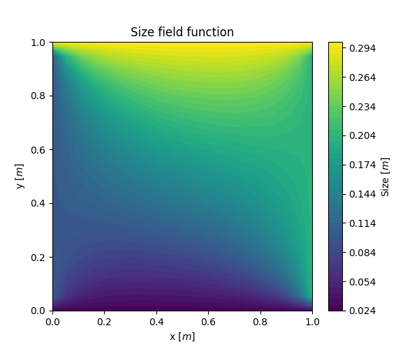
We save this size field function and are now ready to insert points at random locations in [katex]x[/katex] and [katex]y[/katex]. These inserted points will be constrained by the size field function to ensure we have a mesh where the size between elements changes smoothly. Take a look at the mesh generated around an airfoil below, for example:
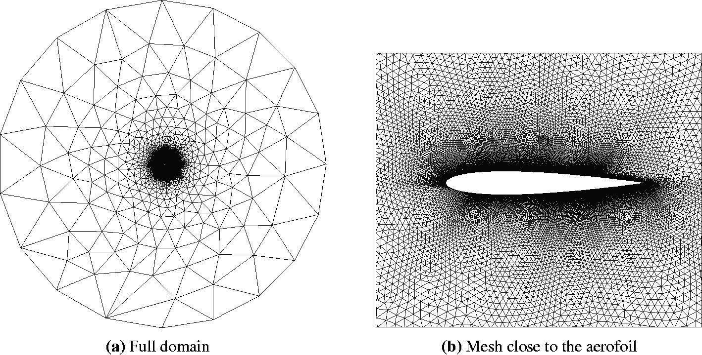
Here, we can see the size field function being applied during mesh generation. On the left, we can see the entire domain and how elements get smaller as we approach the airfoil. A close-up view is provided on the right, showing the mesh around the airfoil itself. Thus, the size field provides us with a mechanism to easily blend between different grid spacings on boundaries (e.g. here the far field and the airfoil), and whenever you see a grid like this, it is likely that a size field function was used in the background.
OK, we now also know how to generate points, let's finally review how to generate unstructured grids out of these points using either the Delaunay or advancing front algorithms.
The Delaunay algorithm
Finally, we have arrived at our first unstructured mesh generation algorithm, and it is a classic! I can't quite decide if I should celebrate it as one of the most popular mesh generation algorithms out there, or if it is time to put the Delaunay algorithm into the history books and remember it as the workhorse of complex CFD algorithms that it once was. Perhaps we are somewhere in between.
No doubt, the Delaunay algorithm has driven a lot of the simulations of industrial complex cases in the past decades, but mesh generation for CFD applications has advanced, and it is my feeling, or hunch (which I cannot back up with literature, facts, or numbers), that the usage of the Delaunay algorithm is on the decline, based on the algorithms I see implemented in mesh generators nowadays.
Certainly, in areas like computational geometry, the Delaunay algorithm is a quick and cheap way of generating a triangulation of random points in 2D or 3D space, and it is heavily used here. But, for CFD applications, we have found more sophisticated algorithms, and therefore we see the Delaunay algorithms less and less.
In any case, as I will show later, once we have a triangular (2D) or tetrahedral (3D) mesh, we can use this as an input to generate the so-called Voronoi diagram, which will generate arbitrarily-shaped polygons (2D) or polyhedra (3D). So, even if we want to make use of some more advanced meshing concepts (e.g. polyhedral cells), we still need to find an initial triangular or tetrahedral mesh as an input to generate some more advanced grids.
When we talked about structured mesh generation algorithms, in particular, hyperbolic and elliptic mesh generation, we derived the PDEs and saw that they automatically try to maximise the orthogonality, that is, grid lines that cross should, whenever possible, meet at a normal (90 degree) angle. Unstructured mesh generation is no different.
Since the Delaunay algorithm can only generate triangular (2D) or tetrahedral (3D) grids, we can limit ourselves to these two basic elements without loss of generality (that is o. B. d. A. for my 6% of German readers, you are welcome) and start to think of properties of a triangle. In this case, we can, for example, easily compute the equilateral skewness for a 2D triangle and see how we can generalise this.
Let's remind ourselves what the equiangle skewness states. It states that the skewness is lowest if all angles within a triangle are the same. This angle is known as the equiangle, and, for a triangle, we know that all angles summed up are equal to [katex]180^\circ[/katex], and so the equiangle must be [katex]\theta_e = 180^\circ / 3 = 60^\circ[/katex]. Once we start to deviate from this angle, we start to get some skewness. The larger the difference between angles in a triangle and the equiangle, the greater the skewness.
You may notice that this definition is somewhat difficult to extend to 3D. Now we have angles in 3D space, and each vertex is connecting 3 edges. While we could compute the angle for each edge pair, we don't really care what the angle is. The points are given to us from the domain nodalisation, and at least at this stage, we don't want to move them (we may apply some smoothing later and move nodes around). What we want to do is connect all points with triangles in a way that minimises the skewness in all cells.
In a nutshell, this is what the Delaunay algorithm is doing; you could think of it as an optimisation strategy as well, if you want. The way the Delaunay algorithm minimises the skewness is through a geometric test. In 2D, we are dealing with triangles (which consist of 3 vertices), and in 3D, we are dealing with tetrahedra (which consist of 4 vertices). We can uniquely determine a circle in 2D by using 3 points, and we can uniquely determine a sphere in 3D by using 4 points.
Thus, all we are doing, really, is to draw circles (in 2D) or spheres (in 3D), as is shown in the following schematic drawing:
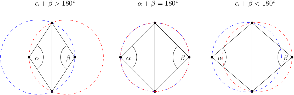
What I have shown here are two triangles that share a face in the middle. I have also indicated two angles, [katex]\alpha[/katex] and [katex]\beta[/katex], which are located opposite to the shared face within each triangle. Now I am placing a circle through each triangle by using all of its vertices. Notice what happens. If [katex]\alpha + \beta \gt 180^\circ[/katex], then each circle will not just contain the vertices they are made up from, but also the vertex from the adjacent triangle.
If, however, [katex]\alpha + \beta \lt 180^\circ[/katex], then each circle will only contain the three vertices it was made from. As it turns out, these skinnier triangles are better for reducing skewness. Let's see why. In the following, I have drawn two triangle pairs for the same 4 points, as seen in the following schematic drawing:
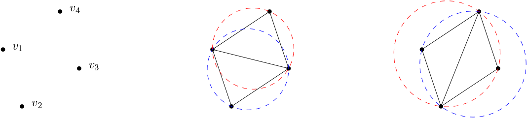
For the case shown in the middle, the circles contain only their own three vertices ([katex]\alpha + \beta \lt 180^\circ[/katex]), while for the case seen on the right, each circle contains one additional vertex from the adjacent triangle ([katex]\alpha + \beta \gt 180^\circ[/katex]). Now look at each triangle pair and determine which of these will have the smallest overall angle.
The triangulation shown on the right will have the smallest angle at the shared face. These angles look to be close to [katex]45^\circ[/katex]. By simply flipping the diagonal, i.e. the shared face in the middle, we obtain the triangulation as seen in the middle, where the smallest angle seems to be closer to [katex]60^\circ[/katex], i.e. the equiangle of the triangle.
Thus, whichever triangle combination results in circles only containing their own vertices, we reduce the skewness as seen in the figure above. In the literature, this process is known as the edge swapping algorithm, as we are swapping the edge (shared face) if any circle contains more than 3 vertices. And that is the Delaunay algorithm. All it does is to triangulate some given points (from the domain nodalisation) and test which triangle combination produces the lowest skewness through edge swapping.
I could leave it at that, but we haven't really defined how to generate the triangles in the first place. There are also some special cases we need to consider; otherwise, we will limit ourselves to the grids we can produce.
In the schematic figure shown below, we can see all the steps required to generate an unstructured grid using the Delaunay algorithm, which includes the initial triangulation, as well as the edge swapping:
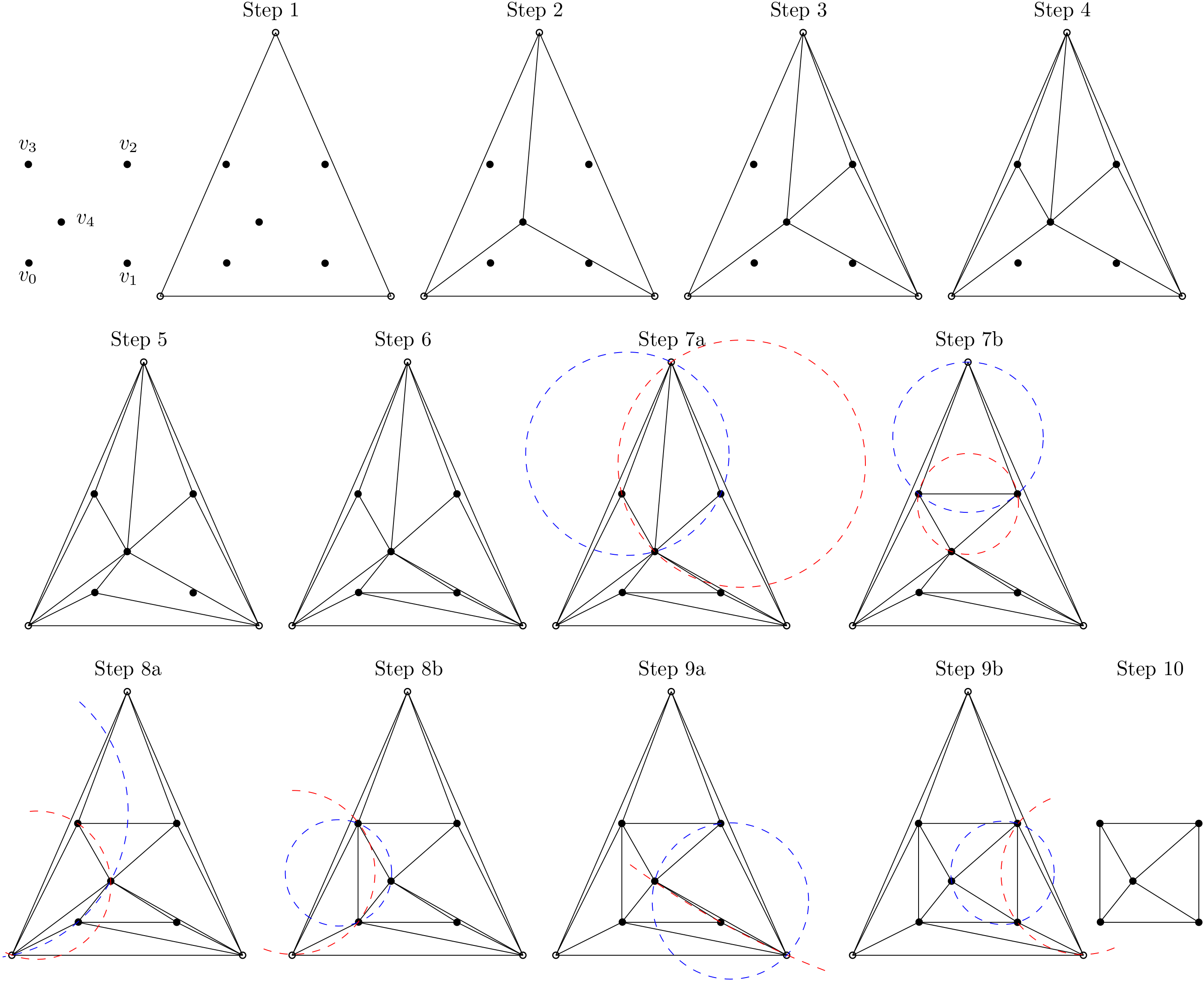
The steps can be summarised as follows:
- Starting with the initial distribution of the vertices within the domain and on the boundary, construct a master triangle which encloses all these vertices (Step 1).
- Next, we select an arbitrary point within the domain or on the boundary and split the master triangle into three smaller triangles, where the randomly selected point becomes a shared vertex for all three triangles (Step 2).
- Now we have to check each of these three triangles to see if it contains additional vertices. If that is the case, we simply select one point at random again, create three new triangles, and repeat the process, i.e. check if any of the newly created triangles contain any further points (steps 3-6).
- Once all triangles have been found, we check if we have to perform an edge swap by placing circles around each triangle. Step 7a-9b shows how this is done for three different triangle pairs. All of these triangle pairs have additional vertices within their circles and thus require an edge swap. It is also shown that once the edge swap is performed, no further vertices are located within the circles. This is always the case.
- Finally, once all edges have been swapped and the best triangulation has been determined, we have to remove any triangle that is made up of at least one vertex that belonged to the master triangle created in the beginning (Step 2). This is shown in Step 10. After the master triangle is removed, the final, triangulated mesh with the lowest global skewness has been obtained.
In this example, I have not specified the boundaries; instead, these were obtained as part of the edge swapping solution, though in general you would want to specify them. This approach works really well if we are dealing with convex domains, but what happens if we have some concave features? Let's look at the following geometry, where the domain is outlined on the left, and the generated mesh is shown on the right:

The Delaunay algorithm has generated triangles outside the domain, which is not what we want. This is a limitation of the algorithm, but one which can be easily overcome by limiting the direction in which triangles can exist. This is shown in the following:

Here, we specify an inside and outside region, and we want to restrict the generation of triangles to the inside region only. The way we can do that is by checking the dot (scalar) product of the normal vector and the vectors that make up the edges of the generated triangles, which in the schematic drawing above are referred to as [katex]e_1[/katex] and [katex]e_2[/katex].
We use the convention here that the normal vector points into the domain. If that is the case, the dot (scalar) product of the normal vector with either [katex]e_1[/katex] or [katex]e_2[/katex] must be positive if the triangle is pointing inside the domain. If the product is negative, then it must be pointing outside, and the triangle must be deleted. This is a quick and easy fix we can apply, making the Delaunay algorithm flexible and robust.
See, unstructured grid generation is easy. No equations (well, almost, at least no lengthy PDEs!), just instructions on how to code the Delaunay algorithm. As we will see, the advancing front method, discussed in the next section, is no different!
The advancing front algorithm
The advancing front method is very different to the Delaunay algorithm, at least in the way we implement it, but it achieves a very similar quality by trying to reduce the skewness as well, though through a different mechanism.
First, though, let us discuss where the name is coming from and what the main principle behind the advancing front method is. For that, let us look at the following schematic overview of the algorithm:

The starting point of the advancing front method is a surface mesh of some description. In the example given above, for example, we have the vertex distribution on the boundaries given by edges [katex]a, b, c, ..., l[/katex]. These edges form the so-called initial front. We also have the internal points given through the domain nodalisation, although these points can also be found through a size function approach by the advancing front method.
With these things given, we go through each edge in the initial front and we snap it to the closest point within the internal domain. Perhaps this makes intuitive sense to you; perhaps it doesn't, so why would we do that? The closest point is defined as the point for which the combined length of the edges that connect to it is minimised. Let's look at an example. The following schematic shows two possible points we could connect to:

We see two initial points on the boundary at the bottom (hollow circles), which then connect to one of two possible points shown on the left and right. I have written the length next to each edge, as well as the angles that are formed inside the triangles. The triangle on the left has a combined edge length (of edges [katex]a,b,c[/katex]) of 12.82 units. The triangle on the right, however, has a combined edge length of 12.06. Thus, it has the shortest combined edge length, and therefore it must be the better triangle choice of the two.
We can see that by inspecting the angles which are formed. For the triangle on the left, the minimal angle is [katex]\theta_{min}=41.2^\circ[/katex]. The max angle is [katex]\theta_{max}=90^\circ[/katex]. For the triangle on the right, however, we have [katex]\theta_{min}=59.4^\circ[/katex] and [katex]\theta_{max}=60.3[/katex]. Let's compute the skewness for these two triangles. As a reminder, the equiangle skewness was defined as:
Q_{skewness}=\max\left(\frac{\theta_{max}-\theta_e}{180^\circ - \theta_e}\, , \,\frac{\theta_e - \theta_{min}}{\theta_e}\right)\tag{134}Here, the equiangle [katex]\theta_e[/katex] is set to [katex]\theta_e = 60^\circ[/katex] for a triangle, i.e. the angle for which we obtain an equilateral triangle. So, for the left as seen in the figure above, we have:
Q_{skewness}=\max\left(\frac{90^\circ-60^\circ}{180^\circ - 60^\circ}\, , \,\frac{60^\circ - 41.2^\circ}{60^\circ}\right) = \max\left(0.25\, , \,0.31\right) = 0.31\tag{135}For the triangle shown on the right, however, we obtain a skewness of:
Q_{skewness}=\max\left(\frac{60.3^\circ-60^\circ}{180^\circ - 60^\circ}\, , \,\frac{60^\circ - 59.4^\circ}{60^\circ}\right) = \max\left(0.0025\, , \,0.01\right) = 0.01\tag{136}While the points haven't moved that much, we see that even a slight change in point movement can have quite a significant influence on the overall mesh quality (i.e. here the skewness). So, the advancing front method will always try to connect some edges of the initial front with the closest point in the internal domain to minimise the skewness.
Let's return to our example we saw before, reproduced below for convenience:
Once we have snapped one initial front (edge) to the internal domain, we repeat this process with the next front (edge). We repeat this process until there is no more edge left in the initial front. The state is shown in the fourth domain from the left in the figure above. At this point, we have generated a new initial front, and we repeat this process, i.e. we snap those edges to the next internal points.
As we do that, we keep track of the triangles that form as a result of our front moving through space. We repeat this process until there are no more points left in the internal domain which are not yet snapped to by the advancing front. Once no vertices are left that have not yet been connected to, and no edges are left inside the advancing front, we have finished the process, and the triangles that have been left behind form the entire grid.
And, by now, you can guess where the name is coming from. Since the front is moving from the boundary towards the interior points, we call the algorithm the advancing front method.
Some mesh generators have extended the advancing front method and offer a quad-dominant version (for 2D surface grids). This has the advantage that we obtain an almost structured-like surface mesh, even for complex geometries, where we obtain good overall orthogonality while retaining geometric flexibility without the trouble of generating a structured grid ourselves.
The following example shows this in action, where I generated a quad-dominant surface grid for the common research model (CRM) by NASA:
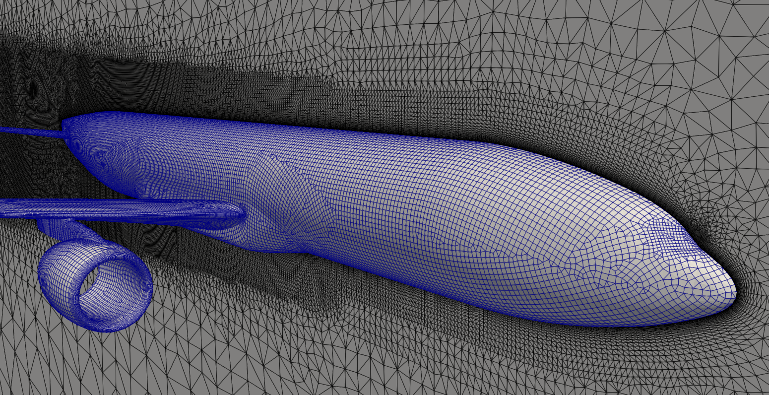
I say quad-dominant; it is not quad-only. If you look closely, you will find a few triangles here and there, especially where fronts are marching towards each other. We may get some local regions where the skewness will spike, but as long as these cells are not introducing excessive skewness and thus false diffusion, we won't really feel the influence of these cells too much.
I'd say the advancing front method is the preferred method these days to generate unstructured grids, especially surface grids. We may then combine these 2D surface grids with either a 3D advancing front method, or, more commonly used, with an octree approach, where we try to retain as many hex elements in the far field as possible. This is the approach taken by many commercial and open-source software generators, where the transition between the surface mesh and the hexa-dominant far field is achieved through polyhedral cells.
So, I mentioned the magic word: polyhedra. Let's see how we can generate these from an unstructured triangular mesh and why this is a good idea in the first place!
From Triangles/Tetrahedra to arbitrary Polygons/Polyhedra
The name of the game is polyhedral cells. The first time I saw them was in StarCCM+'s mesh generator, and as a student, I was intrigued. Why would we ever want to use polygons (2D) or polyhedra (3D) for mesh generation when triangles and tetrahedral elements already give us sufficient geometric flexibility? Well, it all comes down to grid quality.
First, let us see how we can generate a polygon in 2D, from an initial triangular mesh. This is shown in the figure below on the left:

Here, we obtained some triangular mesh, for example, using the Delaunay algorithm, and now we want to create a polygonal grid where the sizes of the edges remain roughly the same. To do that, we first find the centroid of the triangles, and then we connect each triangle's centroid to form a polygon. This is shown in the figure above on the left with the dashed lines. Note how each polygon centres around one vertex that is common for all triangles, which are used to create the polygon.
In 3D, the procedure is exactly the same, but we would use the centroids of tetrahedral elements, and the resulting shape would be polyhedral elements. We can always generate these polygons or polyhedra from an initial triangular or tetrahedral mesh, and these polygons/polyhedra are also called the Voronoi diagram. Some more sophisticated people, who presumably raise their pinky finger while sipping tea, also call this the dual graph of the Delaunay triangulation.
I mention these words here because you will hear them in the literature. If you hear Voronoi diagram, or dual graph of the Delaunay triangulation, think: converting triangles/tetrahedra to polygons/polyhedra. Of course, this terminology carries a bit more mathematical meaning with it, and I am simplifying here a bit, but for our purposes, it is fine to see it this way.
So why would we want to ever create polygons or polyhedra? Well, look at the triangles again in the mesh above on the left; they don't really boast the highest quality. Look at the triangles at the bottom right: we have high skewness here, as well as high area ratios. On the right side of the figure, I have removed the triangles and only shown the polygons, as well as the vectors connecting the centroids of the polygons with one another.
We can see that, overall, we do get a good quality. The area between polygons doesn't change as drastically as for the triangles, and the vector connecting the centroids is almost normal in most cases, with the face that is shared between centroids. This means that we will get a good orthogonality for these cells. Thus, the reason to opt for polyhedral cells is that they can turn a poor-quality triangular mesh into a high-quality polygonal mesh (in 2D, but the same holds for 3D).
There is one misconception, though, that I often hear from my students. If you generate a polygonal or polyhedral mesh, you will see that despite keeping edges about the same length, your number of cells will reduce drastically, typically around a factor of 2 to 4, if you had a pure triangular/tetrahedral mesh before and you convert it to a pure polygonal/polyhedral mesh. This is then often taken as a reduction in computational cost.
This makes sense on the surface, until you implement your own CFD solver and realise that the number of cells has nothing to do with the computational cost. We don't loop over the number of cells, but rather over the number of internal faces. CFD solvers tend to be face-based (we perform the operation at the faces) and not cell-based (where operations are performed at cell centroids).
Take the finite volume method, which we need to use for unstructured grids (well, or the finite element method). In the finite volume method, we are concerned with fluxes that leave or enter our cell, and we typically transform our volume (cell-based) integrals into surface (face-based) integrals using the Gauss theorem. So, while it is true that the number of cells has gone down, the number of internal faces has remained approximately constant, and so no gain in computational cost is achieved.
Right, at this point, I think I can't teach you much more about grid generation. If you have followed the article from start to end (really? respect!) and you have found all of my spelling and grammar mistakes, then you should have a really good understanding of how grids are generated in CFD. Perhaps it has inspired you even to start writing your own mesh generator, who knows. In any case, let's wrap up this article and get excited for the next one!
Summary
In this article, we took a deep dive into mesh generation and everything that is important to know about mesh generation. We started by classifying the grids into their different types, e.g. body-fitted, conformal vs. non-conformal, and overset, and then reviewed the most important grid quality metrics. These were the orthogonality, skewness, aspect ratio, and area/volume ratio.
We saw that just a single cell with poor quality metrics can yield either poor convergence, wrong results, or even divergence. Getting a mesh with high quality is important, but also difficult, and most issues in CFD when you run more complex cases come from insufficient grid quality.
We discussed various structured mesh generation approaches and how PDE-based approaches, such as hyperbolic and elliptic grid generation approaches, aim to maximise the orthogonality in the mesh. In general, structured grids are still preferred over unstructured grids, due to their inherent better quality, though significant advances have been made that have closed the gap between structured and unstructured grid generation algorithms in terms of the overall grid quality.
We saw that the classic unstructured grid generation algorithms are the Delaunay and advancing front method. The Delaunay method used to be the working horse of unstructured mesh generation, though the advancing front method seems to be more popular these days. Both methods generate an unstructured triangular or tetrahedral mesh, though some have created a quad-dominant advancing front method that can generate grids that are almost indistinguishable from structured quad-dominant grids.
Furthermore, we saw that any triangular or tetrahedral mesh can be easily transformed into a polygonal or polyhedral mesh using a Voronoi diagram, and we saw how polygonal/polyhedral cells retain the geometric flexibility of triangles/tetrahedra while generally maintaining a better overall quality, which is closer to that of a structured grid in some cases.
While we looked at mesh generation techniques in this article, most of us will interact with mesh generation in the form of software. There are countless mesh generators out there, and most CFD solvers these days ship with their very own, capable mesh generator, making third-party mesh generators almost obsolete, at least if you go with these solvers.
For example, if you go with ANSYS Fluent or StarCCM+, you get a very beefy and excellent mesh generator. And, in the case of Fluent, their mesh generator is actively developed and sees new feature in every release, and the direction in which this software is going shows that ANSYS knows exactly what they want this mesh generator to be and they are doing a fine job of making this one of the best mesh generators out there (well, my view, anyways).
StarCCM+ has had a pretty good mesh generator itself, and they had it long before ANSYS started to add a mesh generator into Fluent directly (of course, they had other mesh generators before). In any case, if you are using either of these two software, you will be fine. If you are using OpenFOAM and snappyHexMesh, my condolences!
Third-party mesh generators become more important these days if you write your own solver and you want to generate your grids externally. Typically, this would be the case in a research environment, and so having access to a good third-party mesh generator would make sense here.
Regardless of which software you use, you have to put in the time to get to know your software in order to generate high-quality grids. You have to know how to inspect your generated grids and how to visualise the grid quality, and then use that to guide you in improving your mesh locally. If you generate a mesh and never check its quality, you are essentially driving a car blindfolded; a crash is all but inevitable.
The analogy I use in class is this: I can tell you all I want about how to play the guitar and music theory, but unless you practice, practice, and then practice some more, you will never become a world-class guitar player. The same is true for mesh generation; if you want to become a world-class CFD practitioner, you have to practice generating grids, and you have to know your tools (software). If you don't, you won't be able to go beyond simple simulation or even worse, depend on others to generate grids for you.
If you have come all the way to the end of this article, then I take it that you are committed. Make it a goal to become proficient in mesh generation, or, if you already are, become the go-to expert in mesh generation so that we are not limited by our grids to run the simulations we want. In my guesstimation, 95% of all CFD-related issues can be traced back to grids with poor quality. Let us work together on reducing this number so that we can run complex cases with confidence and solve the toughest challenges of tomorrow using CFD!
Acknowledgements
Special thanks to Alexander Schukmann, and Ben Cullen for helping me to improve this article! Check out how you can contribute, too.
Tom-Robin Teschner is a senior lecturer in computational fluid dynamics and course director for the MSc in computational fluid dynamics and the MSc in aerospace computational engineering at Cranfield University.