Why is everyone switching to GPU computing in CFD?
Any serious general-purpose CFD solver these days offers some form of support for graphics processing units (GPUs), be it accelerating the linear solver to speed up the computation of [katex]\mathbf{Ax}=\mathbf{b}[/katex], or by offering a native GPU solver where the entire CFD solver is running on the GPU. The trend is going towards having native GPU solvers, and solvers that are currently only using GPUs for some tasks see an ever-increasing tighter integration into other parts of the CFD-solving process as well.
GPUs have a unique hardware architecture that is related to central processing units (CPUs), but they differ in a few key aspects, which makes them so powerful. In this article, we will explore what these key differences are and why they make GPUs so powerful. By the end of this article, you will understand where this power comes from, both from a hardware and coding (parallelisation) point of view. GPUs will only become more important in the future and as a serious CFD practitioner you need to understand at least the basics, see this article as your introduction.
In this article
The rise of graphics processing units (GPUs) in CFD
If you haven't lived under a rock for the past years, then you'll have noticed a steady increase in CFD solvers trying to leverage the power of GPUs. ANSYS Fluent has introduced their native GPU solver over the past years, growing in capabilities in each release, Siemen's Star-CCM+ has followed and offered GPU support since its 2022 release, SimFlow has ported OpenFOAM to GPUs (though this development seems stagnant at the time of writing this article), and Numeca has started to add support for GPUs to their solvers as well.
So what's this sudden increase in GPUs all about? First things first, when we talk about graphics processing units (GPUs), or more generally, General purpose GPUs (GPGPUs), I am referring to graphic cards. The most well-known company in this domain is without a doubt Nvidia, and as of Summer 2024, it is the most valued public company, surpassing giants such as Microsoft, Apple, Google, and, yes, even cfd.university!
But let's go back in time a bit. When I was looking to build my first PC in the mid 1990s, a high-spec, high-end PC would cost a small fortune, and even then, it would have been less powerful than any modern smartphone. I remember having a dual disk set-up, with the primary disk boosting a staggering 8 GBs of storage, with a secondary data disk of 2 GBs. My smartphone now has 1 TB of storage, how times have changed.
Back then, my first PC had a central processing unit (CPU) clock frequency of 233 MHz. Yes, this was a somewhat of a budget option, but even the most powerful chips were only reaching around 500 MHz. Back then, we needed to buy specialised magazines to stay up to date with hardware development, and if memory serves me correctly, the constant main stories were around developments to get CPUs past the 1 GHz barrier.
CPUs were king, and it was all about getting that CPU speed up to ever larger clock frequencies. Moore's law stated that the number of transistors on a CPU chip would double every two years due to improved manufacturing techniques, thereby increasing the clock frequency, and this was true for a period between 1975 to approximately 2020, after which the law has been declared as dead.
Though, while the number of transistors may no longer double, what we are seeing instead is an increase in compute power through more and more CPUs working in parallel. If we inspect the peak performance of high-performance compute (HPC) clusters, published by the top500 list (listing the top 500 performing HPC clusters world-wide), we can see a steady increase in compute power. This continued increase in computing power is often seen as an extension of Moore's law, especially in the high-performance scientific computing community.
In the 1990s, we were living through exciting times, witnessing the breakthrough of the 1 GHz barrier in CPUs (and, to a gaming kid like myself at the time, it was probably just as important as for some who sat through the moon landing or breaking the speed barrier). By the end of the decade, the AMD Athlon chip finally broke the 1 GHz barrier, and AMD and Intel were battling over the coming years for consumers. AMD was believed to have a far superior chip compared to Intel, but Intel had a larger marketing budget, so their battle continued.
While everyone was focusing on the CPU battle and their rise to clock frequencies of around 3 - 4 GHz (where they have stagnated), Nvidia built graphic cards specifically aimed at gamers. Having a fast CPU was just one part of the equation, but you needed to have a decent GPU to get those mouth-watering 30 frames per second (FPS) playing counter strike (or whatever else was popular at the time, I wouldn't know, I spend all of my time in Microsoft Flight Simulator 95 and 98, what a time to be alive! See for yourself):
If you wanted to impress your friends with these stunning graphics, you had to invest in a decent graphic card, and Nvidia's GeForce series was likely the most popular one among gamers (and probably still is today!).
There was just one metric gamers cared about, and that was frames per second, i.e. how many times per second could your graphic card refresh the screen to give you a stutter-free experience? It was rather common to make compromises in the graphics settings to get somewhere between 15-30 FPS. No one cared about the hardware, really, it was all about that magic FPS number, and gaming benchmarks on different graphic cards were printed in pretty much any PC magazine at that time.
That all changed in 2006 when Nvidia quietly released their software development toolkit (SDK), which they called the Compute Unified Device Architecture, or CUDA, in short. It didn't make waves, it didn't cause people to break down walls and proclaim a revolution, it was just a piece of software that Nvidia provided to programmers to start programming on GPUs, instead of CPUs. Little did Nvidia know that this release would ultimately see them become the most valued company in the world, all through the power of code!
CUDA provided programmers essentially with two things; copying data to and from your PC's main memory to the GPU's memory (which brings about some complication as GPU memory is different to plain CPU memory) and a way to execute code on the GPU specifying how many threads, or workers, should execute your code in parallel. If you look at CUDA programming, that is really all you need to master, and it doesn't get more complicated than that.
All of a sudden, your average script kiddie could take a break from trying to hack the FBI and develop some code that could run on their graphic card. If you were interested in speed, then you were in for a surprise! GPUs were fast, and I mean really fast! I remember playing around with it for the first time in 2014, parallelising a simple 1D CFD solver. Running on a single CPU took about 12 seconds (not bad), but my naive CUDA implementation brought that down to 0.3 seconds! And that was without any fine-tuning of parameters or experience.
When I first saw those results, I got a rush of adrenaline (or, perhaps, it was just a result of my lack of vitamin D thanks to the cold German December nights), but I still remember that night and how my perception of GPU computing changed. I could see how this can revolutionise CFD, and 10 years later, we are seeing big CFD companies putting their efforts into GPU computing (I am not even starting to talk about Machine Learning here, which arguably is the main driver behind uptake in GPU computing).
So, in 1947 we saw the breaking of the sound barrier, in 1969 we saw the first man on the moon, in 1999 we got the first 1 GHz CPU and now, in 2024, we are living through a GPU revolution that touches many areas of lives, and increasingly the CFD community. So in this article, I want to look at this hype and explain why people are jumping on the GPU hype train to give some perspective. Hopefully, this article will give you enough appetite to try GPU computing yourself, or at least put that gaming GPU you have to use to run some CFD simulations on it!
(and yes, I know that comparing the GPU revolution with the first moon landing or breaking of the sound barrier is a silly comparison, but then again, I am a silly man)
Hardware considerations
In this section, I want to review a few key concepts so that we have a shared understanding of the hardware that goes into building a laptop, PC, or indeed a HPC cluster. There are a few components we need to understand that combined with some other concepts will reveal why GPUs are so powerful.
Clock frequency
The most important metric a CPU is judged on is its base clock frequency. This number will tell you how many operations your CPU can perform per second. So if you have a 3 GHz CPU with 4 cores, each core can execute 3 000 000 000 operations per second. If you can utilise all 4 cores to 100% of their potential, you can see 12 000 000 000 operations per second done on your data (obviously, this isn't realistic, you still need to have some operations left for the operating system and background processes to run, but you get the idea).
That is a large number. By operations, I mean how many instructions a CPU can do. Most CPUs will have a standard fetch-decode-execute cycle, where each of these 3 instructions is one operation. In a nutshell, fetching refers to getting an instruction on what to do, e.g. read memory, go to a function, add two numbers, set a pointer address, delete memory, etc. Decode will translate that instruction into a form that CPU understands (e.g. how to set its transistors), and execute will then perform that action.
Through clever pipelining of this fetch, decode, and execute statements, we can actually achieve three operations in parallel, further increasing speed by a factor of, well, three.
There is a limit of how high your clock frequency can go, and typically 4 GHz is a good number to remember. We need to place more and more transistors on a CPU to get a higher clock frequency, and that is achieved by placing transistors closer and closer together. There is a physical limit how close these can get, which we reach at about 4 GHz. It is possible to place them closer, but that comes at an exponentially increasing price.
Power required
One aspect more commonly ignored is the power required to run a CPU (or GPU) at its clock frequency. The power required is computed using the following formula
P=P_{dynamic}+P_{short-circuit}+P_{leakage}[katex]P_{dynamic}[/katex] is a direct measure of your CPU usage. If you run compute-intensive CFD tasks, [katex]P_{dynamic}[/katex] goes up. If you are browsing the internet instead, this number (and CPU usage) remains low. The other two components relate to the micro-scale effect at the transistor level, which we do not have control over, and are related to its design and manufacturing. I won't go into more detail here about these two components, as they are not relevant to our discussion, but you can read up on them using this source.
Let's take a look, then, at [katex]P_{dynamic}[/katex], which is given as:
P_{dynamic} = CV^2fHere, [katex]V[/katex] is the voltage, [katex]f[/katex] the clock frequency of your CPU, and [katex]C[/katex] a load capacity, which typically is difficult to estimate. However, there are two important take-away messages in this equation
- The power required varies linearly with the clock frequency
- The power required varies quadratically with the voltage
There is a slight complication, though, and that is that the frequency itself is a function of the voltage as well. That makes sense. If you want to use more of your CPU's computing capability, you need to support it with more voltage to run at an elevated level of performance. Thus, increasing clock frequency also results in an increase in voltage. So, while the equation above suggests a linear increase in power with increases in the clock frequency, the hidden dependence of the clock frequency on the voltage makes that a quadratic trend instead.
This is important and we will come back to that in a second, but for now, the only thing you need to take away from this is that increasing the clock frequency results in a quadratic increase in the power required. If you want to read up more on this, there is a rather nice explanation of this on the physics' stackexchange site, which also elaborates on the dependence of the clock frequency on the voltage, and how to estimate that.
Hardware architectures
Let's examine the architecture of CPUs and GPUs in more detail. We'll need this to appreciate how the different design philosophies affect the overall performance and so in this section we'll contrast CPUs with GPUs. Let's look at CPUs first.
CPU
The image below shows the architecture of a CPU and is likely the type of architecture your device has that you are currently using to read this article. If you are one of my few exotic readers who read this website on their mobile (hello!), you'll likely have an ARM chip instead of the more common x64/x86 architecture that I'll look at below. In that case, ignore the L1 cache and the rest of the discussion should be true for your chip as well. See, this is an inclusive community; I don't discriminate against chips!
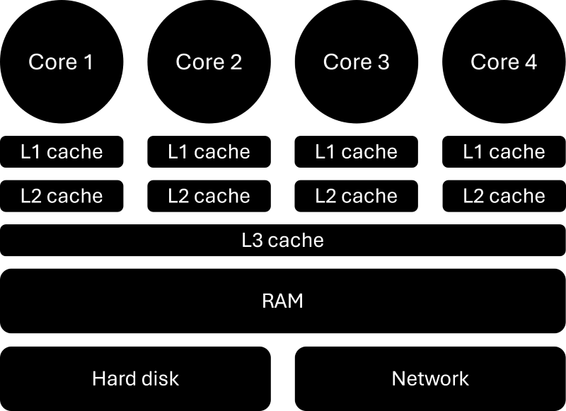
We see that our system can (and typical does) have more than a single core. Each core operates at its own base frequency and may be utilised differently by the operating system. Each core has its own L1 and L2 cache, which are small units of storage that the core is using to fetch memory from the main memory (i.e. RAM). The RAM itself is separated from the L1 and L2 by a shared L3 cache, which all cores have access to.
As we go from hard disk to RAM, from RAM to L1/L2/L3 caches, and finally from our caches to registers sitting within each core (not shown here, but each core has its own private memory called registers), we decrease the time it takes to read and write memory, which comes at the cost of decreasing the size of each memory unit. I have talked at length about caches in my article on memory management, which you may want to check out for additional insights. In there, you will find the following image:

This image shows the access time for each storage unit, as well as the typical maximum storage capacity. We see that as storage size decreases, access time becomes faster. If you gave your car keys to a valet parking service and they parked somewhere you didn't know, how long do you think it would take you to find it yourself in a car park of 1, 10, 100, and 1000 cars? Clearly, the smaller the car park, the faster you'll find your car, and the same is true for memory. We make it smaller, and it gets easier to find the memory we are looking for.
To understand why this would be beneficial (and indeed is a necessary evil), let's take a CPU with a clock frequency of 3 GHz. If you can perform 3 000 000 000 operations per second, that means that each operation will take 1 / 3 000 000 000 seconds, or approximately 0.33 nanoseconds (ns). If we look at the registers shown in the image above, we see that the access time happens to be 0.3 ns as well. Thus, memory in registers can be read within one clock cycle.
If we had to access memory directly from RAM or hard disk instead, without a cache and register hierarchy in-between, it would take approximately 62.9 ns / 0.3 ns = 210 or 0.1 ms / 0.3 ns = 100 ns / 0.3 ns = 333 clock cycles to get memory from RAM or our hard disk, respectively, every time we requested it. Thus, if we had code like:
double a = 1.0;
double b = 2.5;
double c = a + b;
std::cout << c << std::endl;
We would be waiting for 210 or 333 clock cycles to execute line 1 (writing memory to main memory) and the same for line 2. Line 3 involves 3 memory operations (two reads, one write), so 630 or 999 clock cycles and line 4 would be one memory reading operation, so again, 210 or 333 clock cycles. This is a somewhat simplistic view, but it gives you a rough idea of how long this would take.
If we divide our 3 GHz by 210 or 333, we roughly get 0.01 GHz or 10 MHz. The first 10 MHz chip was introduced in 1975. Clearly, that was not a time in history we remember as being known for its fast processors, and we don't want to limit ourselves to 10 MHz computing power! So, we need caches.
Just as an aside; the combination of all of your cores plus the L1, L2, and L3 register is known as the central processing unit (i.e. the CPU). Sometimes people say that they have 4 CPUs in their PC when they really ought to be saying that they have a single CPU with 4 processors or cores. It is a small semantic distinction, but now you can pretend to be a computer science guru, you are welcome!
GPU
The GPU is not all that different to a CPU. A schematic of its architecture is shown below:

The basic building block is a streaming multiprocessor or SM. This is somewhat akin to a CPU, i.e. we have a collection of cores (for Nvidia graphics cards, we call them CUDA cores), and all of these SMs have their own constant cache, shared memory, as well as an L1 cache. Why do we have shared memory? Well, the naming is perhaps somewhat confusing (as the other memory types are shared as well), but shared memory is shared among different SMs, while constant and L1 memory is local to each SM (as shown by the arrows).
This brings me to the next point: GPUs have a lot of streaming multi-processors, consumer graphic cards these days typically have tens of SMs (e.g. 16, 32, or 64 SM), and 128 CUDA cores per SM (you can do the calculation in your head now and see how GPUs have far more cores than CPUs).
On your GPU, you have an L2 cache, which is shared among all your SMs, as well as a global memory (which is akin to RAM) and a special texture memory space (I'll let you guess what this memory bay is used for in the context of consumer gaming graphic cards ... (but we can use it as well if we want)).
Then, the GPU is connected to the host device (i.e. your PC's or laptop's motherboard, typically through a PCIe interface. So, if you want to run code that lives on your host (which it does, as we compile our code on our PC / laptop and then store it somewhere on our hard disk), we need to copy it first to our GPU. If we are writing our GPU-enabled code, it will always run on the CPU, and we, as programmers, have to explicitly state which memory should be copied to the global GPU memory and which functions should be executed on the GPU. This is what CUDA allows us to do.
Differences between CPUs and GPUs
Now that we understand the basic architecture of CPUs and GPUs let's look at what makes them different. Both CPUs and GPUs have a base clock frequency and an associated power required to run each core. A CPU is designed to work on single tasks sequentially, as fast as it can, while a GPU is designed to work in parallel, on a large number of points in a data set, with a lower base clock frequency. Jamie and Adam from Mythbusters have done a neat job of comparing CPUs and GPUs in a more visual manner, which is worth the 90-second watch time:
This design approach is on purpose; a CPU has to work on sequential tasks like opening a program, reading a text file, allowing for changes to take place, writing the changes back to memory, etc. All of these steps have to be performed one after the other, so we want them to be done as fast as possible.
A GPU, on the other hand, was designed for graphic visualisations and was initially driven by gaming needs. Your screen has a certain resolution (e.g. 1920 by 1080 pixels, or a total of approximately 2 million pixels), which means to get a smooth gaming experience, we need to have a device that can perform many costly operations in parallel and lots of them in parallel. This is what the GPU is doing. Lots of operations are in parallel, but in a direct comparison of a single core on a CPU and GPU, the CPU will always be faster.
If we take a quick detour to OpenGL, the programming framework of choice for creating 3D scenes, we will see that it allows you to draw triangles to the screen and apply either colours or textures to them. This is all you need to visualise an entire game (or CFD post-processing application, for that matter!).
Creating a 3D scene typically involves an object generated in some CAD or 3D rendering software, which has its own coordinate space. But then you place it inside a so-called world (or 3D scene), which has its own coordinate space. Then you have a camera looking at the 3D scene, which has its own coordinate system. Finally, you want to have some form of parallel or perspective projection, which will require some transformation of an existing coordinate space into a corrected one.
All of these transformations - going from one coordinate system to another - require a vector matrix multiplication (think back to your linear algebra lessons, and you may remember coordinate transformations; if not, here is a handy overview). We have to do this matrix-vector multiplication a few times (going from one coordinate system to another) whenever something changes for each pixel (approximately 2 million), and, for our gaming friends, we should be doing this 60 times per second. That amounts to approximately 360 million operations per second.
That's a lot, but it also only covers the update stage. We haven't discussed computing other things in the background, which will likely take equally as much time. So, if we can offload this work to the GPU, our CPU is free to compute collisions, physics updates, handle controller input and audio cues, etc.
Thanks to these gaming needs, we now have GPUs that are powerful devices, and this is the appeal for porting CFD solvers to GPUs; you are likely to have an Nvidia GPU anyways on your machine, and if you do, you may as well use it for your CFD calculations and enjoy the additional compute power available to you! So let's have a look at the main differences between CPUs and GPUs in terms of clock speed and available cores:
- CPUs: They have a clock frequency of around 3 - 4 GHz these days and typically have 4 cores per CPU. Some may have 8 - 30 cores, though these are more commonly found in workstation PCs.
- GPUs: They have a clock frequency of around 1 - 2 GHz but make up for their decreased clock frequency in the number of cores as we saw. A modern (gaming) GPU will typically have around 1000 - 2000 cores (16 SMs * 128 CUDA core/SM = 2048 CUDA cores), while high-end GPUs specifically aimed at scientific computing can have as many as 5000 - 10 000 cores.
So, GPUs use a lower clock frequency (and thus physically smaller cores), which gives them space to put a ridiculous number of cores on their chip. But this is just one aspect of why GPU computing has become so popular. We also need to look at different parallelisation strategies to understand why GPUs have a better parallelisation characteristic, which we will look at next.
Before we do, though, I can't finish this section without talking about Intel's Xeon Phi chip, specifically the Knights Landing version (KNL), which was Intel's attempt to rival GPUs in the early 2010s. It had similar clock frequencies to a GPU, around 1 - 2 GHz, while featuring up to 72 cores (it couldn't reach 1000+ cores due to the different architectures of CPUs and GPUs).
The appeal was that you would get a similar level of performance compared to a GPU, which would allow you to run code that was already optimised (and parallelised) on the CPU to continue running without any code modifications. While this was a good idea on the drawing board, the chip lacked memory, had a limited number of applications that would actually benefit from this chip, GPUs were already doing a better job, and intel's own customers were more interested in other Intel products, which saw the Xeon Phi series being finally discontinued in 2020.
A gentle introduction to parallel computing
Since we have reached the end of Moore's law and we can no longer increase the number of transistors (and thus clock frequency) every two years, we have to instead opt for using more cores at the same time to continue to see an increase in compute performance. If we are using more than a single core, we enter the wondrous world of parallel computing, where we have essentially two different parallelisation strategies available:
- The distributed memory approach
- The shared memory approach
Let's take a look at both of them to get an idea what some advantages and disadvantages are for each approach.
Distributed memory approach
Let's start by looking at distributed memory first. The name is derived in the way memory is partitioned, and that makes all the difference in how you have to operate your parallel code. Using the CPU architecture we saw above, I have indicated in the image below what a distributed memory approach would do:
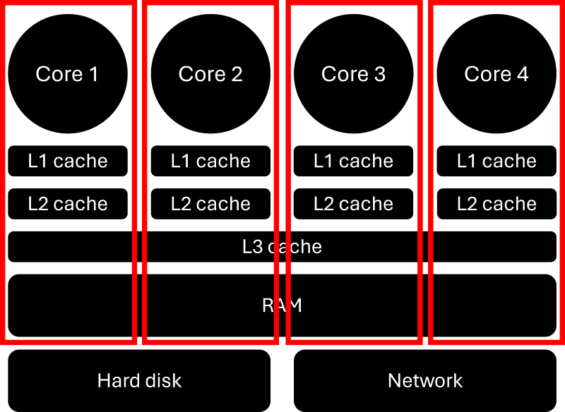
We now say that each core has its own L1 and L2 cache, just as before, but we create barriers on the L3 cache and RAM, which means that each core will have its own private address space on the L3 cache and RAM, which none of the other processors can access. Why is this appealing? Well, if I know how to communicate memory with my neighbouring core and I need some data from it, then it doesn't matter if the core is sitting on the same CPU, the same (or a different) compute node in a cluster, or even somewhere in a geographically different location.
As long as my parallelisation framework knows how to communicate memory across processor boundaries, and it has access to a network connection, then my application can use as many cores as I have available (on a PC, cluster, or distributed network of machines over the internet).
That's great, if I need 2 cores to run my application, or 1 million, it doesn't make a difference. I don't need to change my code if I want to run on different types of PCs or clusters (though you probably need to optimise your code a bit more if you actually need 1 million cores, Amdahl's law will make that painfully clear). This is what all major and commercial CFD solver these days have implemented.
But there is no free lunch so what is the downside with this approach? Well, let's say we have this simplified model equation that we want to solve (linearised Navier-Stokes with no pressure or diffusion, I never claimed it is an interesting equation, but we like it enough in CFD to constantly (ab)use it):
\frac{\partial \phi}{\partial t}+a\frac{\partial \phi}{\partial x}=0If we discretise this with an explicit time integration scheme and upwinding for the spatial term, we get (you can read my article on this equation discretisation if you need some more pointers):
\phi_i^{n+1}=\phi_i^n-a\frac{\Delta t}{\Delta x}\left(\phi_i^{n}-\phi_{i-1}^{n}\right)=0When we launch our parallel application, the first thing we have to do is a domain decomposition step. Let's say we have a domain of 100 points (this is a 1D equation) and we split it into 2 processors, then each sub-domain will receive 50 points and will operate on that separately. Less work per core (50 points instead of 100) results in faster computation. But what if we are exactly on the boundary point?
Let's say we are at the first point on processor 2, which is located at [katex]i=50[/katex]. When we compute [katex]\phi_i^{n+1}[/katex], we can see from the equation above that we need [katex]\phi_{i-1}^{n}[/katex] for that, i.e. [katex]\phi_{i-1}^{n}=\phi_{49}^{n}[/katex], which is located on processor 1. However, since each processor now has its own private memory space, we can't just go to processor 1 and get it, as it may or may not be on the same physical RAM.
So how do we get this value then? Well, we politely ask processor 1 if it would like to share its values with us. This is known as inter-processor communication, and it takes time. It mainly takes time as we now need to share memory on the RAM level, and if you think back to the discussion we had above about caches and RAM, working directly on the RAM is painfully slow for the CPU. You can't do any computations on the CPU while you are exchanging data across processor boundaries, so you want to have as few as possible.
To give you an idea, a really well-optimised Navier-Stokes solver using second-order finite volume methods (e.g. Fluent, Star-CCM+, OpenFOAM, SU2, code_saturne, Numeca, Converge-CFD, etc.) can perhaps operate efficiently with as little as 50 000 - 100 000 cells per processor. If you throw more cores at your problem and you have fewer cells per processor, you are mostly waiting for communication to finish, and your compute time is insignificant compared to your communication time.
So, while distributed memory is great in the flexibility it gives us (i.e. we can run on a single core, 4 cores, or 1 million cores), it doesn't scale well if we throw more and more resources (processors) at our problem. This is why weak scaling is so important when testing CFD solvers, which allows us to establish how many cells we need per core/processor to have an efficient parallelisation approach.
Shared memory approach
Shared memory, on the other hand, is saying that all of this communication is bad. It takes too much time, and we lose a lot of performance, especially if we are only interested in running simulations on a local PC or laptop. In this case, we are throwing away a lot of potential to speed up our code for communicating memory which lives on the same physical CPU. Thus, in a shared memory approach, we leave the RAM shared, and all cores have access to the same memory, as shown in the image below:
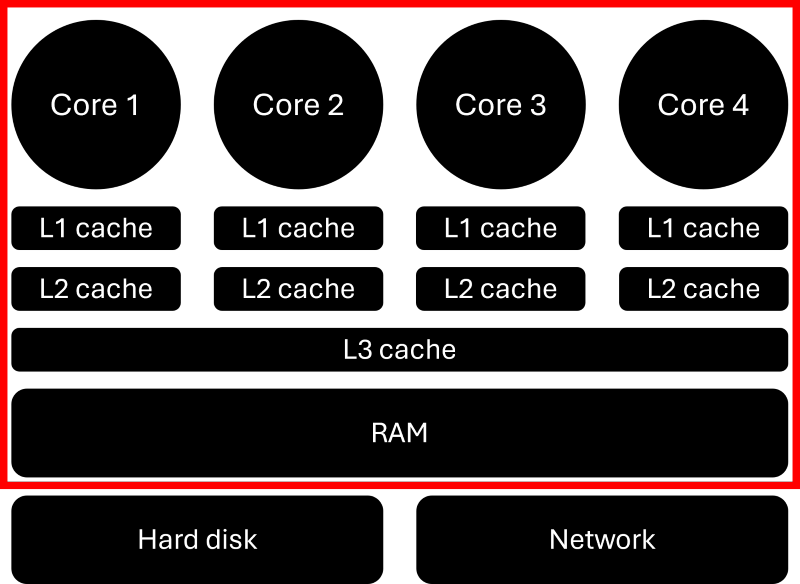
This is obviously better for performance on a single CPU but it also means that you will always be limited to just that single CPU. If you want to go to an HPC cluster, you won't be able to run your code on 1 million cores, as you can with a distributed parallelisation approach. For CFD applications, this may be limiting, but there are a lot of other niches were you will never go to a cluster anyway, in this case, you want to be as efficient on your PC as possible, and this is where shared memory approaches are king.
Now, we can, of course, be savvy and say, why don't we use a shared memory approach within a CPU (or compute node) and then use a distributed memory approach to connect all of these different compute nodes with one another, i.e. we are now using a hybrid shared/distributed memory approach. Yes, we can do that (and many codes that want to stay on the CPU do exactly that). You are asking for trouble, though, as executing a hybrid shared/distributed memory code is not a trivial thing (and requires a cluster of some description).
Common parallelisation frameworks for CFD applications
In this section, let's quickly review common parallelisation frameworks you may find in the wild. I do not intend to explain these in depth, but if you have heard them once, you will later be able to link them back to parallelisation and our discussion in this article.
- MPI: The Message Passing Interface (MPI) is the gold standard in distributed memory parallelisation. It pretty much enjoys a monopoly in the distributed memory category, although alternatives exist. If you are only ever going to learn one parallelisation framework, MPI should be it. Any general-purpose CFD solver that is parallelised uses MPI under the hood. MPI is just a standard (like C++), and we have many different implementations of MPI, e.g. OpenMPI, MPICH, Intel MPI, Microsoft MPI, IBM MPI, and the list goes on (just like we have many different compilers for C++).
- OpenMP: OpenMP is the king in the shared memory approach space, and while not unrivalled, you'll find it used almost exclusively in CFD codes. It is pretty easy to learn, and the best part is you can write both sequential and parallel code at the same time, as OpenMP only uses a specific syntax that will be thrown out by the compiler and thus ignored unless we tell it to interpret these special commands as OpenMP instructions. OpenMP is not to be confused with OpenMPI, which is an implementation of MPI, as seen above. OpenMP now has a mechanism to offload work to GPUs as well.
- OpenACC: OpenACC is somewhat of a clone of OpenMP, i.e. it works very similarly, but the focus was always on GPUs, not so much on CPUs (though it could parallelise on both). Since OpenMP has added GPU support, though, OpenACC has a much tougher time penetrating the CFD market, but similar to OpenMP, it enjoys a pretty user-friendly syntax, and with as little as 3 or 4 additional lines of code, you can offload a large portion of code to your GPU and benefit from its compute capabilities (OpenMP is similar in terms of number of lines required).
- CUDA: As already alluded to above, the Compute Unified Device Architecture (CUDA) is Nvidia's software development toolkit (SDK) that allows us developers to access Nvidia GPUs (of course, you can't access AMD, Intel or any other GPU with CUDA). It is a pretty low-level affair in that you have to write quite a bit of code to get things to work, and you also need to understand GPU architectures well to extract performance. OpenMP and OpenACC are much more higher-level (and at least OpenACC works on non-Nvidia GPUs as well!) and thus quicker to learn.
There are a ton more parallelisation strategies, and originally, this list was much larger. However, I realised that most parallelisation frameworks were not really often if at all, used in a CFD context, so I thought not to bother you with that.
If you have thought along the way: "Hang on, if shared memory approaches are really good within a CPU/node and distributed memory approaches can communicate across nodes, could I not combine these?". You are on to something, and yes, the combination of distributed and shared memory parallelisation strategies is known as hybrid parallelisation approaches, or MPI+X (where the X can be OpenMP, for example). In fact, when it comes to MPI+X, you'll most often find MPI and OpenMP combined together, and this can further accelerate your code.
Putting it all together: What makes GPUs so special?
To understand the power of GPUs, we almost have all the pieces of the puzzle together. The last piece I want to look at is some pseudo-code that will allow us to appreciate where some additional computational efficiency can be gained on a GPU compared to a CPU.
Let's say we want to solve the advection equation as seen in the previous section, then we likely would have code along the following lines:
// include statements

int main() {

  // setting up simulation here
  ...

  // loop over time
  for (int timeStep = 0; timeStep < totalTimeSteps; ++timeStep) {

    // calculate solution at each point on the internal domain, ignoring boundary points
    for (int i = 1; i < domainSize - 1; ++i) {

      // new value of phi at new time level n+1
      phi[i] = phi_old[i] - a * dt / dx * (phi_old[i] - phi_old[i - 1]);
    }
  }

  return 0;
}
Let's look at some pseudo-code that we would have to write to parallelise this code. I am going to gloss over quite a bit of detail here as parallelising code is not difficult, but getting your head around what the code is doing if you have never seen a parallel code is rather confusing, and it would not help in the current discussion.
The following code is the same code using an MPI parallelisation strategy:
// include statements

int main() {

  // setting up simulation here
  ...

  // decompose domain into as many sub-domains as we have processors
  ...

  // loop over time
  for (int timeStep = 0; timeStep < totalTimeSteps; ++timeStep) {

    // get value of phi_old[i - 1] at processor boundary
    double phi_processor = get_processor_boundary_values();

    // calculate solution at each point on the internal domain, ignoring boundary points
    for (int i = 1; i < domainSize - 1; ++i) {

      // new value of phi at new time level n+1
      if (i == 1)
        phi[i] = phi_old[i] - a * dt / dx * (phi_old[i] - phi_processor);
      else
        phi[i] = phi_old[i] - a * dt / dx * (phi_old[i] - phi_old[i - 1]);
    }
  }

  return 0;
}
On line 8, we would have to split our domain first into as many sub-domains as we have processes (i.e. a 1D domain with 100 nodes would have two sub-domains with 50 nodes each if we used 2 processors). On line 15, we request the value that sits on the domain just next to us so we can use this value from the other processor. This is the communication step which is so expensive. On lines 21-24, we either use this received value if i is equal to 1 (i.e. the first iteration, where i-1 would be on the neighbouring processor), or we update the equation as usual otherwise.
Let's contrast that with an OpenMP parallelisation solution:
// include statements

int main() {

  // setting up simulation here
  ...

  // loop over time
  for (int timeStep = 0; timeStep < totalTimeSteps; ++timeStep) {

    // calculate solution at each point on the internal domain, ignoring boundary points
    // OpenMP instruction to parallelise the next spatial loop among a certain number of threads (cores)
    for (int i = 1; i < domainSize - 1; ++i) {

      // new value of phi at new time level n+1
      phi[i] = phi_old[i] - a * dt / dx * (phi_old[i] - phi_old[i - 1]);
    }
  }

  return 0;
}
This looks pretty much like the sequential code, and it should, as OpenMP and sequential codes can live side by side. The only difference is the instruction on line 12. I haven't given the exact OpenMP instruction here, but the point is we issue some specific commands here, and OpenMP will then parallelise the next loop automatically. There is no need to call any costly communication function, as memory is shared, and this is visible to everyone.
Ok, so we have seen distributed memory (MPI) and shared memory (OpenMP) in action. But what about GPUs? Let's look at their code as well (again, in pseudo-code):
// include statements

int main() {

  // setting up simulation here
  ...

  // copy memory from host RAM into GPU RAM
  ...

  // loop over time
  for (int timeStep = 0; timeStep < totalTimeSteps; ++timeStep) {

    // calculate solution at each point on the internal domain, ignoring boundary points
    update_phi<<<16,16>>>()
  }

  // copy memory back from GPU RAM into host RAM
  ...

  return 0;
}
Here, we first copy some memory (i.e. the solution vectors like the velocity, pressure, temperature, etc.) on line 8 from the host RAM to the GPU RAM, which can then be used during the time loop. Instead of writing out the update step for phi explicitly, we capture that in a function (which would have the same content as what we saw in the examples above), only this time it will be invoked with the special <<<N,M>>> syntax, where essentially N and M will determine how many CUDA cores you will use.
There is no hard and fast rule for which values should be set for N and M, and you would likely experiment with them until you get good performance on your device. This is the part I meant where I said you have to understand GPUs to know what values should go in here. It would be a bit too much to go into the details here, as it is not easily explained in a few sentences. But if you want to know more, I'd recommend the crash course by Mark Harris over at Nvidia.
So, if we look at the code, we see that MPI requires costly communication during each time step, whereas OpenMP does not. In CUDA, we also only copy memory once from the host to the GPU memory, and then back once we are done with the simulation. Thus, GPUs are essentially shared memory approaches as well, which means we avoid costly communication.
This copying back and forth, though, can be done in many different ways. CUDA exposes explicit (synchronous and asynchronous), zero-copy, pinned, and unified memory management, all with their advantages and disadvantages. A good overview is given over at codeplay, and if you really want to get lost in memory management, the book Professional CUDA C Programming as reviewed on my CFD reading list is a really excellent book that reviews all of these different approaches along with benchmarking them against one another.
Having said that, the power of GPUs can be expressed by this highly scientific equation:
thousands \ of \ cores \ + \ low \ power \ consumption \ + \ shared \ memory \ parallelisation \ = \ magic!
And, sure, let's say it is magic factorial ([katex]magic![/katex]), why not! This combination is really powerful and the reason why we see so many CFD solvers switching to GPUs as either accelerator (i.e. parallelising only parts of the code which require a lot of computation) or as a native parallelisation approach (i.e. porting the entire solver onto the GPU).
I just want to mention a few things on multi-GPU usage as well, before we close this article. If you want to use 2 or more GPUs, not sitting on the same compute node (within a HPC cluster), you'll have to go back to MPI-X, i.e. now we would have MPI-CUDA. MPI would only send information between GPUs, so they have everything they need.
We said that communicating data between MPI processors is painfully slow, as we are essentially operating directly on RAM rather than caches or registers, which takes about 200 clock cycles, and we need a good number of cells per MPI core to hide this communication cost. With GPUs, this pain is even larger, as we now have to copy memory first from the GPU (RAM) to the host RAM, then copy the data from one MPI process to another, only to then copy that data from the receiving MPI's RAM into its connected GPU's RAM again.
There are some techniques we can utilise here; for example, CUDA-aware MPI may help to soften the pain somewhat, but we have to keep this double memory management burden in mind. Most people, blogs, and even books don't tell you about this, so you'll be left thinking, "Why is not everyone using GPUs all the time?". They do make life more complicated and are more difficult to program, and this gets only worse once we have multiple GPUs. It is worth the pain, though, and this is why we are living through the GPU revolution at the moment.
Summary
We looked at a broad overview of why GPUs are so powerful, and it comes down to raw compute power, low(er) power consumption (compared to CPUs), and an excellent parallelisation approach.
If you are serious about CFD, you owe it to yourself to be at least aware of the power of GPU computing. If you get your hands dirty and actually code up some GPU code, you will get an even better understanding of how GPUs work, what their strengths are, but also where they may not be as good as everyone is making them out to be. You will only ever truly learn how CFD concepts are working (and what their limitations are) if you sit down and code it up. Who knows, we may look at it in more depth again in the future if there is an interest.

Tom-Robin Teschner is a senior lecturer in computational fluid dynamics and course director for the MSc in computational fluid dynamics and the MSc in aerospace computational engineering at Cranfield University.