Advanced RANS and hybrid RANS/LES turbulence modelling in CFD

There is a big gap between classical RANS turbulence modelling and scale-resolving approaches like LES and DNS, both in terms of computational cost and what can be resolved. As a result, classical RANS modelling may be cheap but not always able to resolve the physics we want to capture, while LES and DNS may be able to resolve the physics correctly, but being too expensive to run.

This gap is addressed with advanced RANS modelling approaches, which we will review in this article. First, we will look at RANS models that can capture the transition process (classical RANS models assume the flow to be fully turbulent). This allows to capture the transition between laminar to turbulent flows, which is of vital importance if we are trying to reduce aerodynamic (skin friction) drag. We will look at the two most popular models and also what issues exist that hold transition-based RANS modelling back.

The second approach is concerned with hybrid RANS/LES formulation, where we attempt to mix RANS and LES in a clever way. We try to use RANS in regions where we don’t really need LES-like resolution to reduce the computational cost, while we use LES in areas where it is cheap to run while providing superior quality compared to classical RANS modelling.

We will look at Detached Eddy Simulations (DES), Delayed Detached Eddy Simulations (DDES), Improved Delayed Detached Eddy Simulations (IDDES), Scale-adaptive simulations (SAS), and wall-modelled Large Eddy Simulations (WMLES), which are all approaches that fall into the hybrid RANS/LES category. These represent the latest and greatest advances we have made in turbulence modelling in the last few decades, and they have become widely adopted in academic research and industrial applications alike.

If you have never heard about any of these approaches, or you are just vaguely familiar with them, then this article will give you a deep dive into these topics and elevate your understanding of advanced turbulence modelling. By the end of the article, you will know which approach to use for which situations and how these approaches differ, allowing you to select the most appropriate modelling strategy for your CFD simulations!

In this series

• Part 1: How to Derive the Navier-Stokes Equations: From start to end
• Part 2: What are Hyperbolic, parabolic, and elliptic equations in CFD?
• Part 3: How to discretise the Navier-Stokes equations
• Part 4: Explicit vs. Implicit time integration and the CFL condition
• Part 5: Space and time integration schemes for CFD applications
• Part 6: How to implement boundary conditions in CFD
• Part 7: How to solve incompressible and compressible flows in CFD
• Part 8: The origin of turbulence and Direct Numerical Simulations (DNS)
• Part 9: The introduction to Large Eddy Simulations (LES) I wish I had
• Part 10: All you need to know about RANS turbulence modelling in one article
• Part 11: Advanced RANS and hybrid RANS/LES turbulence modelling in CFD

In this article

Introduction

At this point, we have come quite far in our journey through turbulence modelling in CFD. We started with the origin of turbulence and how to model it using Direct Numerical Simulations. Then, we looked at Large Eddy Simulations, allowing us to reduce the computational cost while retaining most of the DNS resolution, and then at Reynolds averaged Navier-Stokes (RANS) turbulence modelling, which provides a statistical time-averaged sense of turbulence.

At this point, we could say that we have reviewed this matter quite exhaustively (and we have!), but that would be ignoring some breakthroughs in the field of what I will refer to as advanced RANS turbulence modelling. While RANS itself provides a blisteringly quick path to solution compared to LES and DNS, it achieves this with some serious limitations.

For starters, if you have ever done a simulation around an aerofoil, something that should be seemingly simple to set up and run, you will realise that no matter what you do, getting agreement between your predicted drag from CFD and experiments is really difficult to do. The reason is that aerofoils have some laminar flow over the wing, even at very high Reynolds numbers. Laminar flow produces very different viscous drag (due to a different velocity profile in the boundary layer) compared to turbulent flows.

The reason is that RANS models assume the flow to be fully turbulent, and classical RANS models had no mechanism to capture the transition from laminar to fully turbulent. There has been some development on that in the last decades, and it can significantly enhance the predictive power of RANS simulations. This does not come free, though. We typically have to refine our mesh quite substantially and spend more time on validation than we would with a classical RANS model (where no transition is captured).

There is a high uncertainty around transition modelling using RANS and for that reason it has not been applied in the mainstream CFD best practices, however, in cases where the location of the transition within the boundary layer is of importance, or resolving flow physics that require knowledge of laminar to turbulence transition (e.g. laminar separation bubbles), transitional RANS modelling may be an appealing cheaper option than full blown LES or DNS simulations (which are able to predict transition).

Secondly, there has been a very strong research effort on combining the accuracy of LES, especially away from walls, with the computational cheapness of RANS turbulence modelling near solid walls, to get LES-like results with (U) RANS-like computational costs. This approach is known as hybrid RANS-LES turbulence modelling, and you may be more familiar with the terminology Detached Eddy Simulations (DES), which is the most used implementation of this.

Finally, an alternative approach is to use wall-modelling within LES itself to reduce the meshing requirements near solid walls in LES, making computational costs more akin to (U)RANS simulations. This approach is known as wall-modelled LES (WMLES), and it is something that is attracting more and more attention as well.

Thus, in this article, we will be focusing on these developments to make sure we have covered these techniques as well. This will be our final article on turbulence modelling. Let us get started with transition modelling first in the next section.

Going beyond fully turbulent: The transitional RANS models

As alluded to above, having the option of resolving the transition from laminar to turbulent flows may be an appealing feature to have in RANS turbulence modelling. For aeronautical applications in particular, where we are concerned with streamlined aerodynamic surfaces (i.e., trying to reduce pressure drag as much as possible), we will create substantial laminar flow regions. Laminar flow produces smaller viscous drag, and so if we can maximise these laminar flow regions, we can reduce the drag of our aircraft.

Otto Aviation has proposed and developed a business jet that is making use of as many laminar flow-promoting surfaces as possible. Take a look at the prototype they have developed:

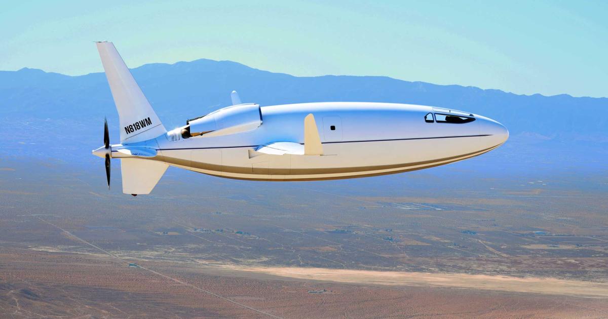
It is making use of NACA 6-series aerofoils, which were developed to promote as much laminar flow as possible. Even the fuselage is shaped in the form of a NACA 6-series aircraft. The propeller is mounted at the rear, pushing the aircraft rather than pulling it through the air (and as a result, flow over the wing and fuselage is largely unaffected by the propeller). There is an interesting discussion on the aerodynamic design of the Celera 500L over at Aviation Stackexchange, which you may want to check for a more detailed discussion.

If we are hired as an aerodynamicist at Otto Aviation and we are tasked with predicting lift and drag for the aircraft, we are in trouble. Classical RANS models, discussed in my previous article on RANS modelling assume the flow to be fully turbulent. As we have established, this will lead to incorrect results in the velocity profile in the boundary layer, and thus, drag predictions.

Thankfully, some turbulence model developers have taken on the burden of introducing a mechanism to distinguish between laminar and fully turbulent flows. As a result, the process of transition can be incorporated into classical RANS models.

In this section, we will look at the two most commonly used models and see how transition is incorporated into RANS modelling.

The Langtry-Menter transition model (\gamma-Re_{\theta,t},\,k-\omega SST)

Ah, we are talking about the first turbulence model, and I am already dropping Menter’s name again. Yes, that is right, Menter, together with Langtry, has given us one of the more popular RANS models that can be used to predict transition. Their model is weird, but from my experience produces the best results of the available transition models. Obviously, this is case-dependent, so your experience may differ.

While the model is weird, it has a certain magic about it, and it is unlike any other turbulence model we have looked at thus far. This is difficult to appreciate if you just look at the equations, so my aim here is to bring these equations to life so we can appreciate what Menter and Langtry came up with.

Let’s put ourselves in their shoes. When Langtry and Menter started their research, there was no serious RANS model available that could handle transition. So they had to invent their own model. Given the popularity of the k-\omega SST model, and the involvement of Menter, it isn’t difficult to see why they picked this model as the starting point. All they had to figure out was how this model could be modified to accommodate transition.

So, let’s look at transition again for a second. Let’s consider the flow over a flat plate and look at the boundary layer that forms. This is shown in the following image:

The boundary layer consists initially of a laminar flow region, which after some point transitions into an intermediate state, the transitional state, after which the flow becomes fully turbulent. There are two characteristic Reynolds numbers here, as shown in the image:

• Re_{c,L}: The critical Reynolds number, where the flow transitions from laminar into the transitional (intermediate) flow state
• Re_{t,L}: The Reynolds number at which the flow becomes fully turbulent.

We always have Re_{c,L} \lt Re_{t,L}. The reference length L is the point along the flat plate at which the flow transitions either into the transitional (i.e., Re_{c,L}) or fully turbulent state (i.e. Re_{t,L}). So how could we codify this into some form of RANS model?

Well, if you have followed my last article on classical RANS models, then you will know that if in doubt, we use a transport equation for an arbitrary quantity we believe represents the flow well.

Ok, so we can probably easily write down the transport equation, but what variables should we be solving for? Well, let’s return to the image above. Langtry and Menter argued that if we model for the critical Reynolds number, i.e., Re_{c,L}, then we know where on a solid surface flow should transition from laminar to turbulent flow. We can then combine this with a variable that indicates if the flow is fully laminar or turbulent, with a value of 0 and 1, respectively. A value between 0 and 1 would then indicate a transitional flow.

This is what they did, and if you are a keen observer, then you would likely find the fundamental flaw with this model immediately. Sure, if we know what Re_{c,L} is on solid walls, this will help us with transition. But what about away from walls? What is the physical significance of Re_{c,L} in the farfield? Well, there is none. We will later see how the transport equation for Re_{c,L} (which will get a different name later) addresses this issue.

So let us then return to the main idea of the Langtry-Menter transition model. We solve the transport equations that we have from the k-\omega SST RANS model, and then we supplement this with two additional transport equations. These solve for the following two properties:

• \gamma: The turbulent intermittency. It is set to 0 in laminar flows and 1 in turbulent flows. Transition can be resolved with \gamma values between 0 and 1.
• Re_{\theta,t}: This is the Reynolds number at which the flow transitions from laminar to turbulent flows. This is essentially the same as Re_{c,L}, with the difference that we use the momentum thickness \theta here instead of some downstream location on a wall, i.e. L. We will see in a bit why this is beneficial.

Let’s look at the intermittency in more detail. It is defined as:

\gamma = \frac{t_{turbulent}}{t_{laminar} + t_{turbulent}}\tag{1}

Here, t_{laminar} and t_{turbulent} are durations for which the flow has been observed to be either laminar or turbulent. For example, if I am in the farfield and there is no turbulence and I measure the flow for a total of 10 seconds, then I likely find that t_{laminar}=10s and t_{turbulent}=0s. Thus, inserting this into the definition above, we get \gamma = (0)/(10 + 0)= 0/10 = 0. Therefore, the flow is fully laminar.

If we are somewhere in the turbulent part of a boundary layer or wake, then we would get, for example, t_{laminar}=0s and t_{turbulent}=10s for the same sampling window of 10 seconds. This would result in \gamma=(10)/(0+10)=10/10=1. Thus, the flow is fully turbulent.

However, in the transition region, we may have the generation of some turbulent spots that will decay and turn into laminar flow again. In this case, we

may have, for example, t_{laminar}=8 and t_{turbulent}=2s, which results in \gamma=(2)/(8 + 2)= 2/10 = 0.2, for the same 10 second sampling period.

Take a look at the following video, which visualises these turbulent spots in the transition region:

Thus, \gamma can be used to determine where we are in the flow (laminar, transitional, or turbulent flow). It is assumed to be zero at solid walls until Re_{\theta,t} is larger than the critical value. At this point, we transition into the transition region and \gamma is allowed to grow until it reaches a value of 1. We will see later how this is achieved by the turbulence model.

OK, this is the main idea behind the model, let’s look at some of the equations that go into the model. At the beginning of this section, I mentioned the critical Reynolds number Re_{c,L}, which is the point along a solid wall where the flow transitions to turbulence. But this isn’t a good Reynolds number to begin with.

This Reynolds number is based on some reference length L downstream of the plate at which transition occurs. This will depend on freestream conditions, as well as the geometry itself. For example, a flat plate may transition later to turbulence than an airfoil, even if the freestream parameters are different (simply because there is curvature on the airfoil). Thus, the value of L is somewhat arbitrary, and if our goal is to create a robust model, we would prefer not to have a dependence on L.

Instead, we may want to reformulate the Reynolds number not in terms of a reference length L but instead based on the momentum thickness \theta. This is defined as:

\theta = \int_0^\delta \frac{u(y)}{U_\infty}\left(1-\frac{u(y)}{U_\infty}\right)\mathrm{d}y
\tag{2}

What does this physically represent? Well, If we integrate along the entire boundary layer profile, we would get a certain momentum. Imagine we want to replace this velocity profile now with a flat velocity profile, but one that has the same integrated momentum. The momentum thickness tells us the height within a boundary layer at which we could replace the velocity profile with a constant velocity profile. We take the velocity at the height of the momentum thickness from the real velocity profile.

This sounds a bit convoluted, so let’s look at this in a sketch:

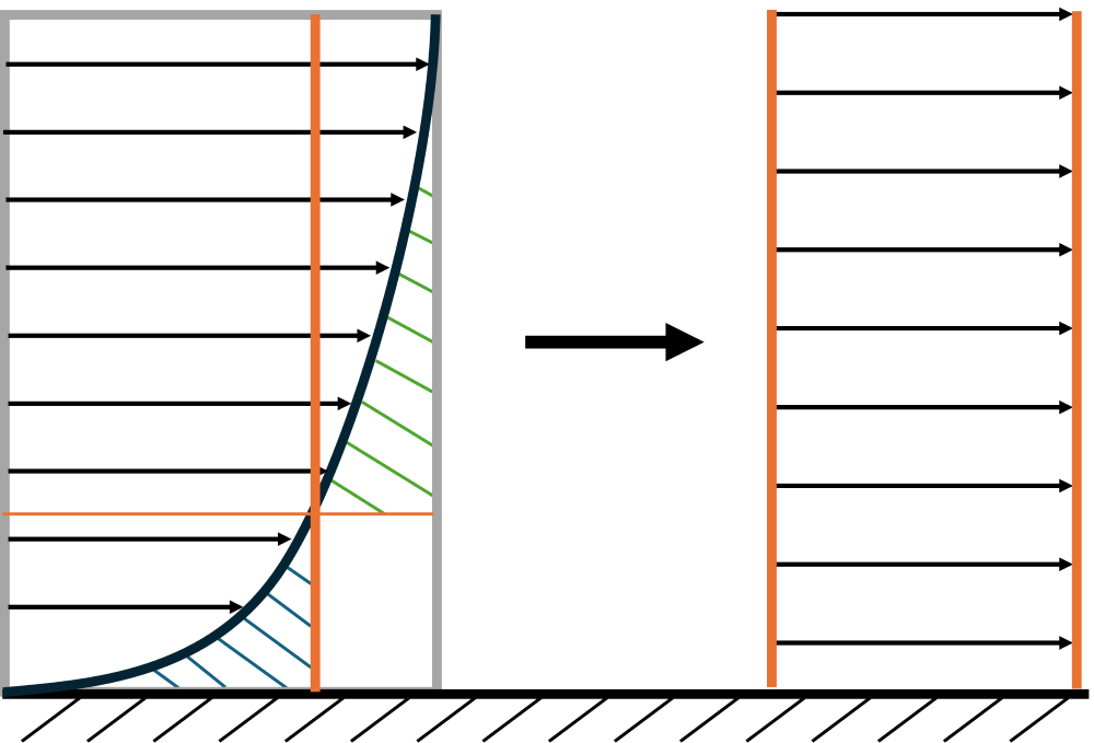
Here, the velocity profile on the right is constant across the boundary layer, whereas the velocity profile on the left (the real velocity profile) has a quadratic or power law shape (depending on the flow regime). Both velocity profiles have the same momentum (\int\rho u(y) \mathrm{d}y).

We see that we can also graphically determine the momentum thickness by placing the entire velocity profile inside a rectangle. We then seek to find a line (shown in orange) that cuts the velocity profile at a point where the green and blue shaded areas are equal.

Ok, so now we’ve got rid of the arbitrary reference length L, job done, right? Well, let’s look at Eq.(2) once more. Notice how we use the definition of the boundary layer thickness to determine the integration bounds, i.e. we integrate from 0 to \delta, where \delta is defined as the point on the velocity profile where we have reached 99% freestream velocity.

This may work for a flat plate, but what if we investigate wake flows? For example, we may want to study the aerodynamic efficiency of a vehicle following another. The second vehicle will be in the turbulent wake of the other. So, the question then becomes, what is \delta here? The second vehicle will experience a mixture of its own turbulent boundary layer and the wake from the leading car. The momentum thickness isn’t clearly defined in this case.

Since we want to write a RANS turbulence model that is robust and can be used for different types of flow, we need to get rid of the \delta dependence. As luck would have it, there is a Reynolds number we can define solely on local flow quantities, which has a strong correlation to the Reynolds number based on the momentum thickness. This is the Reynolds number based on the local vorticity. This is given as:

Re_v=\frac{\rho d^2}{\mu}\bigg|\frac{\mathrm{d}u}{\mathrm{d}y}\bigg|
\tag{3}

Here, we use the velocity gradient near the solid wall. Since a velocity gradient has units of 1/s, we need to square our reference length, which in this case is the distance away from the wall, i.e. d. This definition assumes that we are looking at a flat plate with the y direction in the wall normal direction and the velocity u flowing along the wall. We can mentally replace that by the magnitude of the strain-rate tensor, as we have done so often in previous articles, to generalise this to arbitrary curved geometries.

Let’s plot this vorticity-based Reynolds number along the wall normal direction. This is shown in the following figure:

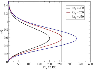
We can see the general shape of the Reynolds number throughout the boundary layer height. This profile is seemingly divided by this magic number 2.193 on the x-axis, why is that? Well, if we look at what the corresponding Reynolds number is, now expressed in terms of the momentum thickness, then we see that scaling the vorticity-based Reynolds number results in its max value to be equivalent to the critical momentum thickness-based Reynolds number. In other words, we have the following functional relationship:

Re_{\theta,t}=\frac{Re_{v,max}}{2.193}\tag{4}

The critical momentum thickness-based Reynolds number, referred to from now on as Re_{\theta,t}, is the point at which the flow transitions from laminar to turbulent flow. Thus, based on local properties, such as the velocity gradient tensor, we can calculate what this transition point will be. We can use this and define a function F_{onset} that will be 0 in regions where the flow is fully laminar, and greater than zero in regions where transition to turbulence should happen.

This function is given as:

F_{onset}\propto\max\left(\frac{Re_{v,max}}{2.193Re_{\theta,t}}-1, 0\right)\tag{5}

We have to subtract 1 from the first argument in the \max() statement to ensure that the value is negative in regions where we have laminar flows. The value of F_{onset} is clipped at 0 so it will never become negative.

Thus, Re_{v,max} is something we can determine from local flow properties at the wall, but what about Re_{\theta,t}? The first question we need to ask ourselves is what this value should depend on? If you look at my discussion on the mechanisms that trigger transition, one such parameter is the turbulent intensity.

This parameter is defined as the fluctuation of the velocity field with respect to the freestream (farfield) velocity. This can be expressed as:

Tu=\frac{u'}{U_\infty}\tag{6}

If we wanted to be a clever dick (of course, we want to be, after all, we talk about turbulence modelling which features the cream de la creme of clever dicks), we could expand the velocity fluctuations as:

u' = \frac{u'+v'+w'}{3} = \sqrt{\frac{u'u'+v'v'+w'w'}{3}}=\sqrt{\frac{2}{3}k}\tag{7}

Here, k is the turbulent kinetic energy, defined as k=0.5(u'u'+v'v'+w'w'). The above assumes that the fluctuations are largely the same in each direction. Well, I said clever dick, but in the end, this expansion is a necessary one, as we do not have information on u', v', or w' in RANS simulations. We do, however, typically know what the turbulent kinetic energy is, and so we can compute the turbulent intensity Tu using the turbulent kinetic energy as:

Tu=\frac{\sqrt{\frac{2}{3}k}}{U_\infty}\tag{8}

Doing some correlation work in the wind tunnel, for simple boundary layer and flat plate cases, we can determine the relationship between the turbulent intensity and the critical Reynolds number at which the flow transitions as:

Re_{\theta,t}=
\begin{cases}
1173.51 - 589.428\cdot Tu \cdot 100 + \frac{0.2196}{(Tu\cdot 100)^2} &Tu \le 1.3\%\\[1em]
\frac{331.5}{(Tu\cdot 100 - 0.5658)^{0.671}} &Tu \gt 1.3\%
\end{cases}
\tag{9}

More advanced formulations are available that also take the pressure gradient into account, which is then expressed as:

\lambda_\theta = \frac{\theta^2}{\mu}\frac{1}{U_\infty}\frac{\mathrm{d}p}{\mathrm{d}x}\tag{10}

For example, Abu-Ghannam and Shaw proposed the following relationship between the critical Reynolds number, the pressure gradient, and the turbulence intensity:

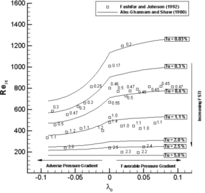
Whichever approach we choose, we need to keep in mind that all these relations make some limiting assumptions that will influence our simulations. While it may be appropriate to determine the critical Reynolds number from the pressure gradient and turbulent intensity for a large number of applications, this may fail to give satisfactory answers for other cases.

For example, looking at the mechanisms that trigger transition again, one such mechanism is cross-flow induced transition. This is not dependent on the pressure gradient (the farfield for aeronautical applications has a constant pressure and thus no gradient), and this transition would still occur with very low turbulent intensities. Clearly, other parameters, related to swirling motions, play a role here which are neglected in these empirical correlations.

But let’s say we are happy that these correlations cover our use case. Then, we know what the critical Reynolds number ought to be from our empirical correlations, and we need to establish the transition length so we know when the flow is fully turbulent. This is done by the F_{length} function, although it does not necessarily provide a length in metres that is equivalent to the real transition length. If anything, it is proportional to the transition length.

This transition length takes a few parameters, the first being a function that calculates the F_{length}^* parameter based on the critical Reynolds number:

F_{length}^*=
\begin{cases}
-119.27\cdot 10^{-4} Re_{\theta,t} - 132.567\cdot 10^{-6} \sqrt{Re_{\theta,t}} + 398.189\cdot 10^{-1}  &0 \le Re_{\theta,t} \lt 400 \\[1em]
-101.695 \cdot 10^{-8}Re_{\theta,t}^3 -123.939 \cdot 10^{-2}Re_{\theta,t} + 194.548\cdot 10^{-5} \sqrt{Re_{\theta,t}} + 263.404   &400\le Re_{\theta,t} \lt 596 \\[1em]
-3\cdot 10^{-4}Re_{\theta,t} + 0.6788  &596 \lt Re_{\theta,t} \le 1200\\[1em]
0.3188  &Re_{\theta,t} \ge 1200
\end{cases}\tag{11}

We need two additional expressions that scale the transition length, which are characteristic of the viscous sublayer. These are given as:

F_{sub}=\exp\left[-\left(\frac{Re_\omega}{200}\right)^2\right]\\[1em]
Re_\omega=\frac{\omega d^2}{\nu}\tag{12}

With this, we are able to compute the transition length that is proportional to the physical transition length but not necessarily equivalent. This is given as:

F_{length}=F_{length}^*(1-F_{sub})+ 40F_{sub}\tag{13}

Let’s take stock of what we have achieved thus far. We have identified a mechanism to compute the local Reynolds number based on the momentum thickness using only local parameters. This allows us to compute the Reynolds number without having to specify a reference length L, and it also allows us to compute a Reynolds number for arbitrary flows.

Now we need to combine this with the transport equations for \gamma and Re_{\theta,t}. Let’s start with \gamma. The transport equation is given as:

\frac{\partial \gamma}{\partial t} + (U\cdot \nabla)\gamma = \nabla\cdot\left[\left(\nu+\frac{\nu_t}{\sigma_\gamma}\right)\nabla\gamma\right] + P_{\gamma 1} - D_{\gamma 1} + P_{\gamma 2} - D_{\gamma 2}
\tag{14}

If you are missing an intuition for what a transport equation looks like, I’d recommend going through my previous article on classical RANS modelling. It will take some time to read, but it is time well spent.

We have our usual terms here for the change in time, advection in space, and diffusion in time. What is different here is that we have two separate production and destruction terms. Typically, RANS models only feature a single production and destruction term, but not this model. Why? Well, \gamma is an indicator of whether the flow is turbulent or not, and there are different mechanisms that can trigger turbulence. Thus, we need more than just a single pair of production and destruction terms.

Let’s look at the first pair, which is the transition onset. We can think of this as the process that models natural transition. Once we have reached a critical Reynolds number, the flow will naturally transition to turbulence. The first production term is given as:

P_{\gamma 1} = 2F_{length}\sqrt{2\mathbf{S}:\mathbf{S}}(\gamma F_{onset})^2\tag{15}

We saw that F_{onset} will become larger than 0 once we are in the transitional flow regime; otherwise, it will be zero for laminar flows, and so the production term will also be zero. It is also scaled by the F_{length} function, meaning a larger transition length will create turbulence faster (higher production of \gamma). Finally, we multiply by the magnitude of the strain-rate tensor, meaning that the strength of the mean flow gradients will also scale the production term. Stronger gradients will result in more production of \gamma and thus faster transition to turbulence.

The destruction term also has some interesting features. It is given as:

D_{\gamma 1}= \gamma P_{\gamma 1}\tag{16}

We simply scale it by the production term. Let’s think about some conditions that can happen:

• If the flow is laminar, then we have \gamma = 0 and so the destruction term must be zero as well.
• For fully turbulent flows, we have \gamma = 1.0 and so production and dissipation are exactly match. This means any \gamma that is created will immediately destroyed, creating an equilibrium condition for fully turbulent flows.
• Only in cases where the flow is between laminar and turbulent, i.e. 0 \lt \gamma \lt 1, we have more production than destruction, since the destruction term is scaled by \gamma. By definition, it must therefore be smaller than the production term. Thus, \gamma can only be created in the transition region. Once it reaches a value of 1, it will stay at 1.

The second pair of production/destruction relates to relaminarisation. Flow can locally become turbulent but then may experience not sufficient energy to sustain that turbulent motion, and the flow will become laminar again. The second production term will be able to capture this behaviour, which allows this model to capture/model laminar separation bubbles, where this phenomenon occurs.

Given that Menter has an extensive history with NASA, which in turn are quite keenly interested in aerospace applications, it is not difficult to see why this second term was included. The production term is given as:

P_{\gamma 2}=c_{a2}\Omega d F_{turb}\tag{17}

with the corresponding destruction term

E_{\gamma 2} = c_{e2}\gamma P_{gamma 2}\tag{18}

Here, we need to define the additional functional relationship:

F_{turb}= e^{-\frac{k}{4\nu\omega}}\tag{19}

So what have we gained here? \Omega is the vorticity tensor and \omega is the specific dissipation rate, which is only non-zero close to solid walls. In the farfield, \omega is close to zero, making F_{turb} go to zero in the farfield but to non-zero values near solid walls (e.g. where laminar separation bubbles would be located). We use the same trick here with the destruction term, i.e. it is scaled by the production term and \gamma.

Let’s talk about the elephant in the room, then. I have left the best for last, and by that, I mean the critical Reynolds number Re_{\theta,t}. The transport equation for it is given as:

\frac{\partial Re_{\theta,t}}{\partial t} + (\mathbf{u}\cdot \nabla)Re_{\theta,t} = \nabla\cdot\left[\sigma_{\theta,t}\left(\nu+\nu_t\right)\nabla Re_{\theta,t}\right] + P_{\theta t}
\tag{20}

Let’s just appreciate how ridiculous this is. The critical Reynolds number Re_{\theta,t} is the Reynolds number which determines where the flow will transition from laminar to turbulent at solid walls. What is the meaning of Re_{\theta,t} in the farfield? There is none! But, we are solving a transport equation, so clearly we will have a value for Re_{\theta,t} everywhere in the domain. Is this a problem?

Well, from a physical point of view, yes, having information about Re_{\theta,t} in the farfield is pointless and of no use. However, from an engineering point of view, we accept that we break our physical understanding of the world every now and then if it suits us (and the results we are getting are not too bad). This is what we are doing here as well.

The transport equation has been designed with some clever mechanisms that allow us to use it and to get good results despite the oddity of using a transport equation for a value that is only required near solid walls.

The way that we make the transport equation for Re_{\theta,t} work for us is in two steps:

• First, we impose the critical Reynolds number as a Dirichlet boundary condition at the inlet. We may know this value from experiments, or we can use an empirical correlation such as given by Eq.(9).
• Second, we enforce this value to be constant in the farfield. Only close to solid walls do we allow it to change so that ti can adjust to local changes in the geometry, e.g. curvature of the wall.

Let’s see how this is achieved through the transport equation given by Eq.(20). We have our usual 3 terms that we have seen in any other transport equation as well. These are responsible for time changes in Re_{\theta,t}, the convection of Re_{\theta,t} from one place to another, as well as the diffusion of Re_{\theta,t} in space. But notice what else is given by Eq.(20), or rather what is absent.

We have a single production term P_{\theta t} but no corresponding destruction term. This is at odds with how we typically construct our transport equations for RANS turbulence models. We usually require that a quantity can be produced or destroyed, but not in this case. So let us look at the production term in more detail. It is given as:

P_{\theta t} = \frac{c_{\theta t}}{\tau}\left(\overline{Re_{\theta t}} - Re_{\theta t}\right)\left(1-F_{\theta t}\right)
\tag{21}

Let’s start at the back. We have a quantity F_{\theta t}, which is given by:

F_{\theta t}=
\begin{cases}
1 & \text{laminar Boundary Layer}\\[1em]
0 & \text{freestream}
\end{cases}\tag{22}

From the turbulent intermittency \gamma, we know that we are in a laminar boundary layer if we have \gamma=0. Therefore, we can determine the value of this function. If we are in a laminar boundary layer, the term inside the last brackets reads \left(1-F_{\theta t}\right)=1-1=0. Therefore, the entire equation is multiplied by 0, making the production term P_{\theta t}=0 in laminar boundary layers. If we are in the farfield, however, this is then switched to zero, so that the production term can be non-zero.

Now, let’s examine the first part of the production term. We have a closure coefficient c_{\theta t} that is constant, as well as a timescale \tau, that is given by:

\tau=\frac{500\nu}{u^2}\tag{23}

Similar to how the Reynolds number is defined, we have here a ratio of the viscous (\nu) to the inviscid (u) forces, multiplied by some arbitrary factor. Thus, you can think of this timescale for how long it would take the flow to return to a state of equilibrium. Here is a simple (mental) experiment you can perform (or go splurging on supplies, this is an experiment you can do at home with the kids, why not …).

Take two equal containers, and fill one of them with water and one with honey. Run your finger through both with the same velocity. Which of these will return to an equilibrium state first? I.e., which of these will go back to a state where no flow is detected in the container? Clearly, honey will return quickly to this state, owing to its high viscosity. Looking at the definition of \tau, we could therefore state, as long as u_{honey}=u_{water}, that \tau_{water}\lt \tau_{honey}.

A higher value of \tau will reduce the time it takes for the flow to return to its equilibrium state, as it is given in the denominator of Eq.(21).

And then, we have the term \overline{Re_{\theta t}} - Re_{\theta t}. Here, \overline{Re_{\theta t}} is the value for Re_{\theta t} that we impose at the inlet, i.e. the value for which we know the flow to transition to turbulence. Re_{\theta t} is the value that is obtained from our transport equation (the literature also sometimes uses the reverse definition, i.e. Re_{\theta t} being the value set at the inlet, and \overline{Re_{\theta t}} solved for by the transport equation).

Thus, if the value of Re_{\theta t} we have solved for is the same as the one imposed at the inlet, the difference \overline{Re_{\theta t}} - Re_{\theta t} must be zero. Therefore, the production term is zero. However, if we have \overline{Re_{\theta t}} \gt Re_{\theta t}, then the computed value for Re_{\theta t} is smaller than \overline{Re_{\theta t}} and so their difference \overline{Re_{\theta t}} - Re_{\theta t} is positive. If \overline{Re_{\theta t}} \lt Re_{\theta t}, then Re_{\theta t} is greater than \overline{Re_{\theta t}}. The difference \overline{Re_{\theta t}} - Re_{\theta t} is now negative.

This, the production term, really, is a hybrid production/destruction term. Depending on how much (or little) of Re_{\theta t} we have produced, we will either add or subtract this difference from the transport equation of Re_{\theta t}. We multiply this difference by the relaxation time scale \tau (or rather, its inverse) to allow fluids to reach equilibrium at different times, proportional to their viscosity. Furthermore, the production term is completely switched off in laminar flow boundary layers.

The second secret of the Re_{\theta t} transport equation is the diffusion itself. We saw in Eq.(21) that the diffusive term is multiplied by \sigma_{\theta,t}, another closure coefficient. The value for \sigma_{\theta,t}, as well as other closure coefficients typically used for the diffusive term in other RANS models, is shown below:

• \sigma_{\theta,t} = 10 (current model, i.e. \gamma-Re_{\theta,t},\,k-\omega SST model)
• \sigma_k = 0.6 (k-\omega model)
• \sigma_\omega = 0.5 (k-\omega model)
• \sigma_{SA} = 1.5 (Spalart-Allmaras model)

As we can see, a value of \sigma_{\theta,t} = 10 is much larger (about one magnitude) than any other diffusive closure coefficients taken from other models. While some model improvements were proposed over the years where \sigma_{\theta,t} has changed, this value shows the importance diffusion plays near solid boundaries.

That is, the flow is advected from the inlet towards solid boundaries, e.g. an airfoil. On its way from the inlet to the solid boundaries, the production term ensures that Re_{\theta t} remains constant. Closer to the solid surfaces (e.g. airfoil), the transport equation for Re_{\theta t} diffuses its value that it got from the inlet around the solid boundary. This process is highlighted for the flow around an airfoil, where we see contours for Re_{\theta t}, both for the farfield and a close-up look near the airfoil:

The inlet condition gets advected close to the airfoil, and then diffusion is taking over, wrapping the values for Re_{\theta t} around the arifoil, like a vacuum pump. In this way, we are able to wrap the airfoil (solid walls) with values for Re_{\theta t} that were imposed at the inlet, which are allowed to locally change based on the geometry’s curvature.

I told you, it is a weird model, but it does work quite well, at least for simple test cases. I haven’t really used it for anything beyond airfoil simulations, and there are reasons why you may not either. I will pick up these issues when we talk about the meshing requirements for transitional RANS models.

Having established now the two additional transport equations we need to solve in the \gamma-Re_{\theta,t},\,k-\omega SST model, it is time to combine these results with the standard k-\omega SST model. The standard \omega equation from the k-\omega SST model is used and repeated below for the sake of completeness:

\frac{\partial \omega}{\partial t} + \left(\mathbf{u}\cdot\nabla\right)\omega =
\nabla\cdot\left[\left(\nu+\sigma_\omega\nu_t\right)\nabla \omega\right] + (1-F_1)\sigma_{\omega2}\frac{2}{\omega}\nabla \omega\nabla k +
\frac{\gamma}{\nu_t}P - \beta\omega^2
\tag{24}

However, the transport equation for the turbulent kinetic energy k is modified as shown below:

\frac{\partial k}{\partial t} + (\mathbf{u}\cdot\nabla)k = \nabla\cdot\left[\left(\nu+\sigma^*\nu_t\right)\nabla k\right] + \hat{P}_k - \hat{D}_k
\tag{25}

Here, we are modifying the production and destruction terms. The production term is given as:

\hat{P}_k=\gamma P_k \\[1em]
P_k = \tau^{RANS}:\nabla\mathbf{u}
\tag{26}

Here, we simply multiply the production of turbulent kinetic energy by the value of \gamma. Intuitively speaking, this makes sense. If there is no turbulence, we can produce any, and so where \gamma is zero, the production of turbulent kinetic energy must be zero as well. Turbulence is only generated in the transition regime, i.e. where 0 \gt \gamma \gt 1. The production term does satisfy this requirement. How about the destruction term? Well, it is given as:

\hat{D}_k = \min\left(\max\left(\gamma, 0.1\right), 1.0\right)D_k \\[1em]
D_k = \beta^* k\omega\tag{27}

This is another weird property of the \gamma-Re_{\theta,t},\,k-\omega SST model. As we can see, the lowest value for the destruction that can be obtained is 0.1D_k. The highest is 1.0 D_k. While the highest value makes sense, i.e. this is the same as the destruction term in the original k-\omega SST model, the lowest value does not. Regardless of the flow, there will always be some destruction.

As we have explored in my article on numerical dissipation, we saw that we always need some form of dissipation to stabilise the flow. This could be either due to the fact that we ignored some of the small-scale dissipative effects (due to using a coarse grid), or it could be to dampen the non-linearities in the flow that only get exacerbated by numerical round-off effects. Thus, some dissipation may reduce accuracy, but it will also promote stability of the numerical procedure.

And this is the \gamma-Re_{\theta,t},\,k-\omega SST model in a nutshell. We solve two additional transport equations for the turbulent intermittency \gamma and the critical Reynolds number at which flow ought to transition, i.e. Re_{\theta,t}. With these two additional variables, we know where the flow is locally laminar, where transition takes place, and where the fully turbulent boundary layer is reached. As a result, we hope to get more accurate flow predictions near solid walls, mainly skin friction drag and separation points.

As we have seen, there were some oddities with this model. We impose the critical Reynolds number at the inlet and then hope to advect it close to solid walls. There were a lot of engineering assumptions at play here. Perhaps your background is in physics, or maths, in which case this model may feel more like an engineer went rogue with the laws of physics, but fear not, the CFD community has a model just for you, which we will look at in the next section.

The k - k_l - \omega model

I personally really like the k-k_l-\omega model. I really do. Perhaps this is coming from the fact that the model we looked at in the previous section was my first introduction to transition models. It felt weird, and to this day, whenever I use the \gamma-Re_{\theta,t},\,k-\omega SST model, something just doesn’t feel right.

The k-k_l-\omega model, on the other hand, is firmly rooted in physics. The model attempts to capture transition by modelling the physical process of transition, and all additional terms in the equation can be attributed to a real physical phenomenon that we can observe and measure in real life. So then, what is this more physically inspired transitional model?

The main idea behind the k-k_l-\omega model is that we have two separate kinetic energies:

• k, or k_T: The turbulent kinetic energy per unit mass, formed by the velocity fluctuations, i.e. k=k_T=0.5(u'^{2 + v'}2 + w'^2)
• k_l: The laminar kinetic energy per unit mass, formed by the instantaneous velocities k_l=0.5(u^{2 + v}2 + w^2)

In a laminar flow, we have k_T=0 and k_l\gt 0, for a turbulent flow, we have k_T\gt 0 and k_l = 0, and then for any intermittent flow we have k_T\gt 0 and k_l\gt 0. We can also express the total kinetic energy, k_{TOT}, as k_{TOT} = k_l + k_T. Fun fact, the word TOT translates to death from German to English. I like to think of k_{TOT} to be the lethal or deadly kinetic energy (but I doubt you will find any textbook adopting this terminology anytime soon!).

So, we have two separate kinetic energies. Their sum is the total kinetic energy. The idea is that we model two separate transport equations for both the laminar and turbulent kinetic energy, and so based on the kinetic energy we have, we can distinguish between laminar and turbulent flows. For example, if we have a laminar boundary layer, we could assert this by computing the ratio k_T/k_l. Since there is no turbulent kinetic energy, k_T=0, and the ratio k_T/k_l becomes zero. This is then similar to the quantity \gamma, where a value of \gamma=0 indicates laminar flow.

The reverse, however, is a bit trickier. For a fully turbulent flow, where k_l=0, the ratio k_T/k_l becomes infinity. So we can’t directly compute an equivalent quantity like \gamma with this model, but we can see that we certainly can differentiate between the different regions.

The main question we have to ask ourselves is, how do we model the transfer from laminar to turbulent kinetic energy? Well, let’s have a look at the transport equations for both k_T and k_l. For the turbulent kinetic energy k_T, we have:

\frac{\partial k_T}{\partial t} + (\mathbf{u}\cdot \nabla)k_T = \nabla\cdot\left[\left(\nu+\frac{\alpha_T}{\sigma_k}\right)\nabla k_T\right] + P_{k_T} - \omega k_T - D_T + R_{BP} + R_{NAT}
\tag{28}

And, for the laminar kinetic energy k_l, we have:

\frac{\partial k_l}{\partial t} + (\mathbf{u}\cdot \nabla)k_l = \nabla\cdot\left[\nu\nabla k_l\right] + P_{k_l} - D_T - R_{BP} - R_{NAT}
\tag{29}

Both equations have the standard time derivative, convection, and diffusive terms, as we have seen so many times with other RANS models based on transport equations. However, there are two nuances here:

• The diffusion term in the turbulent kinetic energy contains an effective diffusivity \alpha_T, instead of directly using the turbulent viscosity \nu_T here. This allows the model to have a more refined approach to computing the turbulent viscosity.
• The laminar kinetic energy only depends on, well, the laminar (or physical) viscosity \nu.

We then see the usual suspects, i.e. both equations feature a construction term, as well as an additional term D_T, that is akin to the cross-diffusion term in the k-\omega SST term. While the turbulent kinetic energy k_T features a destruction term, i.e. -\omega k_T, there is no destruction term in the laminar kinetic energy equation for k_l.

If we think about this, this makes sense. Laminar kinetic energy isn’t destroyed, but rather, it is transferred into turbulent kinetic energy. We do have an explicit equation to solve for this, and therefore, we do not need to add a source term to balance the equation, but instead, transfer laminar kinetic energy to the turbulent kinetic energy transport equation, instead of destroying it through a source term.

The turbulent kinetic energy equation, however, does require a source term, as its energy gets eventually converted into heat at the smallest scales, and we do not resolve this explicitly. Instead, we model this dissipative behaviour through the source term. But, if we wanted to, we could create a new transport equation, model the heat dissipation at the smallest scales (which would be challenging since we do not resolve the smallest scales), and transfer any heat dissipation at the smallest scales to this transport equation. In this case, we could get rid of the source term in the k_T equation.

So, how is the energy transfer from the laminar to the turbulent kinetic energy? This is done by the two additional terms R_{BP} and R_{NAT}, which are introduced to model bypass transition and natural transition. Notice how these terms are negative in the k_l equation but positive in the k_T equation.

Thus, if the model detects that bypass or natural transition occurs at the moment, it will reduce the amount of laminar kinetic energy k_l (negative contributions of R_{BP} and R_{NAT}) and add this to the turbulent kinetic energy. This provides a clean mechanism to transfer kinetic energy from one form to the other. Since this transfer appears with the same magnitude but opposite sign, we conserve the total kinetic energy k_{TOT}.

So naturally, the next question we must ask ourselves is, what are these additional source terms? Let us start our discussion on R_{BP}. Walter and Cokljat, the authors of this model, argue that transition starts when turbulence starts growing faster than viscosity can smooth it out.

If we look at turbulence production in RANS equations, we saw previously that the production of turbulence is typically linked to the velocity gradient, specifically, the strain-rate tensor. The strain rate tensor \mathbf{S} has units of 1/s, so a sensible turbulence time scale could be expressed as t_{turbulent}\propto 1/\mathbf{S}. Similarly, the viscous dissipation time scale can be computed based on the viscosity and a length scale (e.g. the eddy size) as t_{viscous}\propto l^2/\nu, purely on dimensional grounds.

Thus, if t_{turbulence}\gt t_{viscous}, then turbulence generation is stronger than the viscous dissipation, and the flow starts to transition to turbulence.

As an analogy, imagine you are trying to light up a barbecue. You have your coals, a source of heat (a lighter), and the environment (potentially some wind gusts). You are trying to transition the coals from a non-lit to a lit state, by exposing the coal to heat. Initially, there will be some resistance by the coal being lit (similar to viscous dissipation).

The heat from your lighter may not be enough to turn the coals on. But, you may either have a favourable gust of wind (or average wind), or you can use blowing to add oxygen yourself. The influx of additional oxygen will energise the heat source and eventually overcome the resistance of the coal to turn on. Similarly, once a sufficient amount of turbulence is being produced, it will overcome the viscous forces and the flow will transition to turbulence.

This process is modelled by the R_{BP} and R_{NAT} source terms, which, as mentioned previously, will switch on either bypass or natural transitions. The R_{BP} transition is modelled as:

R_{BP}=C_R \beta_{BP} k_L \frac{\omega}{f_W}
\tag{30}

Here, \beta_{BP} is the term responsible for checking if the turbulent characteristic timescale has become smaller than the viscous characteristic timescale. It is given by:

\beta_{BP} = 1 - \exp\left(-\frac{\phi_{BP}}{A_{BP}}\right)
\tag{31}

From this expression, we cannot appreciate this fully, but instead, we need to look at the definition of \phi_{BP}, which in turn is given as:

\phi_{BP}=\max\left[\left(\frac{k_T}{\nu\Omega} - C_{BP,crit}, 0\right)\right]\tag{32}

Let’s look at the first term within the \max() statement. Here, we see the turbulent kinetic energy k_T, with units of m^2/s^2. This is divided by the product of \nu\Omega. \nu is the laminar viscosity in units of m^2/s, and \Omega is the vorticity tensor, with units of 1/s. Thus, combining all dimensions, we have a dimensionless expression as the first term.

C_{BP,crit} is set to 1.2, meaning that if the turbulent kinetic energy k_T is 20% larger than the product of the vorticity tensor and viscosity, we get a value that is greater than zero. So, for laminar flow, we have \phi_{BP}=0, but \phi_{BP}\gt 0 for transitional and turbulent flows.

If we look again at Eq.(\ref{eq:eq:beta-bp}), we see that a zero value of \phi_{BP} will result in \beta_{BP}=0, since \exp(1)=0. If \beta_{BP} is zero, then R_{BP}, i.e. Eq.(30), must also be zero. Therefore, no transition will take place. But, if \phi_{BP} is greater than zero, the exponent in Eq.(31) will be less than 1, and so \beta_{BP}\gt 0. Thus, we will start to generate bypass transition as we have R_{BP} \gt 0.

The process for natural transition follows pretty much the same process. We have our source term for R_{NAT} defined as:

R_{NAT}=C_{R,NAT} \beta_{BP} k_L \Omega\tag{33}

Here, \beta_{NAT} determines again whether natural transition occurs or not. This is defined as:

\beta_{NAT} = 1 - \exp\left(-\frac{\phi_{NAT}}{A_{NAT}}\right)\tag{34}

Again, we have a quantity \phi_{NAT} that determines whether the characteristic turbulent timescale is larger than the viscous timescale to promote natural transition. This equation is given by:

\phi_{NAT} = \max\left[\left(Re\Omega - \frac{C_{NAT,crit}}{f_{NAT,crit}}\right), 0\right]\tag{35}

Now we are using the Reynolds number defined by the vorticity tensor (magnitude) to judge whether turbulence production prevails. This Reynolds number is defined as:

Re_\Omega = \frac{d^2 \Omega}{\nu}\tag{36}

We again have a closure coefficient C_{NAT,crit}, as well as an additional function f_{NAT,crit} that determines the threshold for the vorticity-based Reynolds number which needs to be reached for turbulence production to commence.

Thus, we have established what the two source terms R_{BP} and R_{NAT} represent and how they are computed. Once they are non-zero, turbulence production commences, and we add/subtract an equal amount within the laminar and turbulent kinetic energy equation to predict the transition from laminar to turbulent flows.

Finally, let us turn our attention to the \omega transport equation, which will also need to be slightly modified. But let us remind ourselves what the purpose is of the \omega equation. In general, when we talk about RANS turbulence modelling, we need to solve for two additional turbulent quantities to compute a length and velocity scale. This is because we need to obtain a relation for the turbulent viscosity \nu_t, which has units of m^2/s, i.e. a velocity multiplied by a length.

Unless we solve for some form of turbulent viscosity directly (like we do in the Spalart-Allmaras model), we need at least two transport equations that, combined, will yield a value for the turbulent viscosity. In the case of the turbulent kinetic energy and specific dissipation rate, we can simply combine them in the following way to compute the turbulent viscosity \nu_t:

\nu_t=\frac{k_T}{\omega}
\tag{37}

Thus, let us look at how \omega is computed. Its modified transport equation is given by:

\frac{\partial \omega}{\partial t} + (\mathbf{u}\cdot \nabla)\omega = \nabla\cdot\left[\left(\nu+\frac{\alpha_T}{\sigma_\omega}\right)\nabla \omega\right] + c_{\omega 1} \frac{\omega}{k_T} P_{k_T} - c_{\omega 2} \omega^2 + \left(\frac{C_{\omega R}}{f_W} - 1\right)\frac{\omega}{k_T}\left(R_{BP} + R_{NAT}\right) + C_{\omega 3}f_\omega \alpha_T f_W^2 \frac{\sqrt{k_T}}{d^3}
\tag{38}

We have again the time derivative, convection, and diffusion of \omega, as would be expected from any transport equation. But there are some additional terms here which are specifically added for the capturing of transition.

The first term appears on the right-hand side of Eq.(38). This term is:

\left(\frac{C_{\omega R}}{f_W} - 1\right)\frac{\omega}{k_T}\left(R_{BP} + R_{NAT}\right)\tag{39}

This term becomes active once transition is taking place. For laminar flow, this term is zero, since we have R_{BP}=R_{NAT}=0. Its purpose is to increase the value of \omega in the region of transition. If we now look at Eq.(37), we can see that an increase in \omega results in a decrease of \nu_t. This is important, as we don’t want to fully switch on turbulent production when we have transition. This term limits the amount of eddy viscosity being produced.

Eventually, even if R_{BP} and R_{NAT} continue to rise, this term goes to zero as k_T increases. Thus, the role of this term is to provide reduced turbulence production in the transition region.

This term is similar to Eq.(26) in the \gamma-Re_{\theta,t},\,k-\omega SST model, where we scale the production term by the turbulent intermittency, i.e. \hat{P}_k=\gamma P_k. We do this to bring in the production of turbulence gradually. Thus, both turbulence models have a mechanism to gradually introduce turbulence into the flow, which makes sense, given that transition is a gradual transition from laminar to turbulent flows.

The second term in Eq.(38) we need to look at is given as:

C_{\omega 3}f_\omega \alpha_T f_W^2 \frac{\sqrt{k_T}}{d^3}\tag{40}

Here, we have d^3, the distance from the wall, appearing in the denominator. This cubic wall distance relation is here to limit this term to the boundary layer. Its role is to provide an improved prediction of \omega in the boundary layer.

With these modifications, we have now constructed a more physically inspired model that works more like a traditional RANS model. Both the \gamma-Re_{\theta,t},\,k-\omega SST and k-k_l-\omega model are popular transition models and in use in transitional RANS predictions.

If you followed the discussion up to this point, you may ask yourself why we haven’t all switched to transitional RANS modelling. Why would anyone in their right mind continue to use classical RANS models, which, on paper, seem inferior? Well, classical RANS models have one winning advantage that transitional RANS models can’t compete with. For that, we need to talk about meshing.

Meshing requirements for transitional RANS models

Traditional, or classical RANS models, i.e. those that assume the flow to be fully turbulent (and, as a result, cannot distinguish between laminar and turbulent flows), have pretty relaxed meshing requirements. In terms of the y^+ value, we can set almost any value we want. Nowadays, all RANS models that are implemented in commercial or widely used open-source solvers can work with either a wall-modelled or wall-resolved approach.

In the wall-resolved approach, we target a y^+ value of 1 everywhere at solid walls. This allows us to fully resolve the turbulent boundary layer. However, we can also opt for a wall-modelled approach, where the y^+ value may be somewhere between 30 to 300. It may even be larger if we do not particularly care about accurate gradients at the wall.

For transitional RNAS modelling, however, things are slightly different. The consensus in the literature seems to be that a very fine wall-resolved grid needs to be constructed. Typically, this means that we want to achieve y^+=0.1. Then, we want to grow the cells away from the wall, but with a very small expansion ratio. For classical RANS models, an expansion ratio may be set anywhere between 1.2 and 2, i.e. each cell that is layered on top of another cell, growing away from the wall, may be anywhere between 20%-100% larger than the previous cell.

For transitional RANS models, this expansion ratio is also typically set to a much stricter value of 1.05, i.e. each cell growing away from the wall will be only about 5% larger than the previous cell. This means that the computational cost for transitional RANS models is so large that they become almost unusable.

To make matters worse, if you look at LES, you have far less stringent meshing requirements (at least in the wall-normal direction), and transition is naturally captured. Granted, LES needs to be treated as an unsteady simulation, but if we were to use a transitional RANS model in unsteady mode, we may have slower performance than LES, due to an increased mesh resolution near the wall, while not getting as accurate results as LES near walls, depending on the subgrid scale model used.

For this reason, there are only very few places where transitional RANS makes sense to be used. You will unlikely find it in the wild being used for complex industrial applications, although it cannot be ruled out that transitional RANS models may provide superior results for some applications, which justify their computational cost.

Having said that, I want to leave the world of pure RANS models behind and now start looking at hybrid RANS-LES models, which have exploded in popularity since they were first introduced. Let us do just that in the next section.

When RANS isn’t enough: hybrid RANS-LES models

There is just one final item left on our to-do list, and these are hybrid RANS-LES methods. As alluded to above, these models are the latest and greatest in CFD turbulence research, and if you want to make a name for yourself in the field of CFD and turbulence modelling, this is likely the place you want to focus on.

The idea behind hybrid RANS-LES models is very simple: Use LES whenever feasible but switch to RANS if the grid requirements become prohibitively large for LES. All issues that arise in turbulence modelling are due to one single item: solid walls. Yes, a flow that has no solid walls is so trivial, that you can run a full-blown LES, possibly even a (coarse) DNS, on your microwave’s microchip (honestly these machines are getting too powerful, my microwave decided yesterday that I would have no more food unless I verified that I was the owner by entering a PIN on my mobile).

One of my PhD students did all of his LES work on a standard laptop (no fancy hardware), and those simulations would typically take about 1.5 hours to run. A DNS would be entirely feasible for the same geometry, perhaps taking a day or so. The case we were looking at was the Taylor-Green vortex problem, and this is just a box with periodic boundary conditions where a specific initial condition is allowed to freely evolve.

But, once you throw a wall into the mix, all of a sudden you’ve opened Pandora’s box, out of which the devil emerges, and all of a sudden you have to deal with this pesky little thing called a turbulent boundary layer. Now, you have to spend some serious time considering what grid resolution you should be aiming for, if that would work with your chosen turbulence modelling approach, and potentially if CFD is really right for you in the first place or if you should have done something with marketing instead.

But let’s assume you aren’t easily scared by turbulence, let’s have a look at what hybrid RANS-LES models are and which approaches have been established in the literature. Specifically, we will look at:

• Detached Eddy Simulations (DES) and derivatives (DDES, IDDES)
• Scale-adaptive Simulations (SAS)
• Wall-modelled LES (WMLES)

But first, let us do a head-to-head comparison of RANS and LES and see what their main difference is.

A head-to-head comparison between RANS and LES

In my article on RANS turbulence modelling, we looked at how we can derive the time-averaged, or Reynolds-averaged Navier-Stokes (RANS) equations. We saw that by using the Reynolds decomposition, which decomposes a flow variable \phi into its mean (\bar{\phi}) and fluctuation (\phi') component, and applying that to our momentum equation, we obtain the following time-averaged momentum equation:

\frac{\partial \bar{\mathbf{u}}}{\partial t} + (\bar{\mathbf{u}}\cdot\nabla)\bar{\mathbf{u}} = -\frac{1}{\rho}\nabla\bar{p} + \nu\nabla^2 \bar{\mathbf{u}} + \nabla\cdot\tau^{RANS}
\tag{41}

Here, \tau^{RANS} is the Reynolds stress tensor. In my article on Large Eddy Simulations (LES), on the other hand, we looked at how to derive the spatial-averaged Navier-Stokes equations, which resulted in:

\frac{\partial \bar{\mathbf{u}}}{\partial t} + (\bar{\mathbf{u}}\cdot\nabla)\bar{\mathbf{u}} = -\frac{1}{\rho}\nabla\bar{p} + \nu\nabla^2 \bar{\mathbf{u}} + \nabla\cdot\tau^{SGS}
\tag{42}

Here, the additional stresses \tau^{SGS} are the subgrid-scale stresses that are not resolved by LES. Thus, conceptually, the main difference between RANS and LES is that we take a time-averaged view of our flow field in RANS, while we retain the time history in LES, but we introduce spatial averaging so that we obtain a local averaged view of the flow field in space.

These are two very different approaches, but if we look at Eq.(41) and Eq.(42), and we pretend for a second that we do not know anything about Navier-Stokes, CFD, or fluid dynamics in general, then we would say that these equations are identical, with the difference in notation for the stress tensor, i.e. one equation uses \tau^{RANS}, the other uses \tau^{SGS}.

However, if we look at their definition, we would see that they encode different information. For RANS, we have:

\tau^{RANS} = -\overline{\mathbf{u}'\mathbf{u}'}
\tag{43}

This stress tensor contains the fluctuating velocity components that are not resolved by the flow. In LES, on the other hand, we have:

\tau^{SGS} = \left(\bar{\mathbf{u}}\bar{\mathbf{u}} - \overline{\bar{\mathbf{u}}\bar{\mathbf{u}}}\right)
+ \left(-\overline{\bar{\mathbf{u}}\mathbf{u}'} - \overline{\mathbf{u}'\bar{\mathbf{u}}}\right)
+ \left(-\overline{\mathbf{u}'\mathbf{u}'}\right)
\tag{44}

This contains the velocity components of the resolved velocity (\bar{\mathbf{u}}) and unresolved (\mathbf{u}') velocity field. In both RANS and LES, the stress tensor represents stresses we cannot resolve, i.e. in RANS it is the velocity fluctuations that we no longer resolve with our time-averaged view on the flow, while in LES it is the fluctuating velocity of eddies that are smaller than our grid spacing. Thus, we need to use some form of modelling to find approximate values for both \tau^{RANS} and \tau^{SGS}.

As it turns out, both approaches make use of Bousinesq’s eddy viscosity hypothesis. Granted, there are a few different ways to approximate the stresses, for example, in RANS we may use the Shear Stress Transport (SST) idea of Bradshaw instead which is famously used in the k-\omega SST model, but for the most part, Boussinesq’s eddy viscosity is used by most turbulence models.

So, even if we see that the exact definition for \tau^{RANS} (Eq.(43)) and \tau^{SGS} (Eq.(44)) is very different, we decide to model both terms in the same way. Thus, for RANS, we have:

\tau^{RANS} \approx -2\mu_t\mathbf{S}+\frac{2}{3}k\delta_{ij}
\tag{45}

For LES, on the other hand, we have:

\tau^{SGS} \approx -2\mu_t\mathbf{S}
\tag{46}

Now, you may be saying that these equations are not the same. However, their final form is just different. They are both based on the same eddy viscosity assumption, and the second term we can see in Eq.(45), i.e. (2/3)k\delta_{ij} is written in a different form for LES and typically absorbed into the pressure. So, it is not visible in Eq.(46), but it is accounted for in the modelling. If you want to see how, you can check my write-up on how the Navier-Stokes equations are filtered in LES.

Thus, we can see that both RANS and LES share essentially the same mathematical equations. From an exact mathematical point of view, the unresolved stresses are different. However, we most commonly model these unresolved stresses with the same closure in both RANS and LES, making both approaches essentially the same.

They are not identical, though, as we use different grid requirements in RANS and LES. This will lead to a different resolution and accuracy for both methods, but also to a different computational cost.

Thus, if both RANS and LES are so similar, can we potentially mix their description? Yes, of course, and this will lead us to hybrid RANS-LES models. The idea is to stick to LES whenever the grid resolution is good enough, but once we approach a solid wall, we simply switch to a RANS description, allowing us to use a lot fewer computational cells within the turbulent boundary layer.

If you think that the computational savings for hybrid RANS-LES is due to the reduced number of cells in the boundary layer, you would only be partially right. In fact, the biggest time saving is achieved somewhere else. Given that LES is necessarily time-dependent, i.e. we have to run transient simulations, we have to determine a suitable time step.

In CFD, we typically use the CFL number to determine a stable time step. As we saw in my article on explicit and implicit time integration techniques, the CFL number is really just a non-dimensional time step and is defined as:

CFL=\frac{u\Delta t}{\Delta x}\tag{47}

Solving this for the time step \Delta t, we obtain:

\Delta t = \frac{CFL \Delta x}{u}\tag{48}

If we now consider a flow that we want to simulate with both LES and a hybrid RANS-LES approach, then we can say that the velocity we compute in both cases should be the same. Thus, the velocity u will be the same. We further set the CFL number to be the same in both simulations. Since we have much stricter grid requirements in LES, we will get much smaller cells in LES close to the wall. Therefore, the value for \Delta x will be smaller in LES than for RANS, or hybrid RANS-LES, where we can use RANS grid requirements near solid walls.

We can therefore say that, in general, we have:

\Delta t^{LES} \ll \Delta t^{RANS}\tag{49}

Thus, if we want to advance both solutions in time until a certain total time T, given that LES’ time step is much smaller than the time step in RANS, or hybrid RANS-LES, we have to perform fewer time steps in total to reach the final time T. Since we can only parallelise our solution in space, not in time (although this is an area that is receiving some research as well), our main bottleneck in LES is that we have to compute a lot of time steps that cannot be parallelised.

Even if we have a supercomputer available, all that it can do for us is to make the simulation time per time step as small as possible, but we still have to perform more time steps compared to pure RANS or hybrid RANS-LES to reach T. Therefore, hybrid RANS-LES is actually gaining most of its computational advantage not by reducing the mesh size, but rather by reducing the number of time steps required to advance a solution in time.

However, this discussion only considers the CFL number. For example, if we have an explicit time stepping, then we are limited to a CFL number of one, typically. In this case, hybrid RANS-LES will perform better than LES alone. If we use a fully implicit solver, we could bump up the CFL number for LES to get somewhat faster computation in time, at the cost of smearing the solution in time.

However, there are cases where the numerics are not the limiting factor. For example, let’s say we deal with combustion processes and we want to model the formation of CO_2. For combustion, we need to take the chemistry into account, and typically, chemical reactions happen at a time scale which is much lower than what our CFL number is giving us. We could express that as:

\Delta t^{chemistry} \ll \Delta t^{LES}(CFL=1) \ll \Delta t^{RANS}(CFL=1) \tag{50}

Thus, in this case, we would have to run both the hybrid RANS-LES and the pure LES simulation at the same time step, as this is now governed by the chemical reactions. In this case, there is no computational advantage of using hybrid RANS-LES over LES. In fact, if we only deal with the combustion process, and not the entire geometry of a combustion chamber, for example, we may not even have any solid walls to resolve. In this case, we would typically stick to LES.

Various ways have been formulated in the literature for hybrid RANS-LES models, and we will look at the three most commonly used methods. Let us start with arguably the most common and most popular method: Detached Eddy Simulations and its variants.

Detached-eddy simulations (DES)

Detached Eddy Simulations, or DES, was introduced by Spalart in 1997, so it has been around for quite some time. The main idea behind DES, as a hybrid RANS-LES approach, is that we solve the RANS equations everywhere in the flow, but we change the definition for the turbulence length scale computation locally based on where we are in the flow.

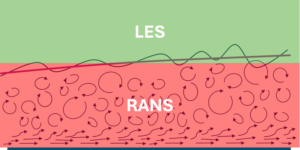
Within the turbulent boundary layer, we compute the turbulent length scale as we would in a classical RANS model, and then, in the farfield, the turbulent length scale is computed as in LES in the farfield. This is shown schematically in the following figure:

Thus, all we need to do is to find a suitable RANS model and modify its turbulent length scale. If you were Spalart in 1997, having just introduced your celebrated Spalart-Allmaras turbulence model a few years earlier, which turbulence model would you choose? Of course, your own! Thus, the very first DES model which was introduced was the Spalart-Allmaras DES model, or SA-DES model. Let us review the transport equation for the Spalart-Allmaras model again. It is given as:

\frac{\partial \tilde{\nu}}{\partial t} + (\mathbf{u}\cdot\nabla)\tilde{\nu} = \frac{1}{\sigma}\nabla\cdot[(\nu+\tilde{\nu})\nabla\tilde{\nu}] + \frac{c_{b2}}{\sigma}\nabla\tilde{\nu}\cdot\nabla\tilde{\nu} + c_{b1}(1-f_{t2})\tilde{S}\tilde{\nu} + f_{f2}\frac{c_{b1}}{\kappa^2}\left(\frac{\tilde{\nu}}{d}\right)^2-c_{w1}f_w\left(\frac{\tilde{\nu}}{d}\right)^2
\tag{80}

Here, we see that both the fourth and fifth term on the right depend on the variable 1/d, where d is the distance to the closest solid wall. These terms were introduced by Spalart and Allmaras to model the effect of solid walls; that is, close to the wall, turbulent eddies are elongated due to the presence of the wall. These terms supply additional correction to the computation of the turbulent viscosity \nu_t, which is directly proportional to \tilde{\nu}, as computed by the Spalart-Allmaras model.

However, as we move into the farfield, the fourth and fifth terms become very small and are effectively removed. This makes sense; the turbulent eddies are no longer deformed by any solid wall. However, it also means that away from walls the destruction terms for \tilde{\nu} essentially go to zero (fourth and fifth term on the right-hand side of Eq.(80)). The production term, the third term on the right-hand side, is therefore not balanced.

This works for RANS, as our grid is typically much coarser than LES, as we only want to resolve time-averaged flow properties. Therefore, \tilde{S}, which is used in the production term on the right side, will be fairly constant (time-averaged). If there are no mean flow gradients (which is typically the case for flows far away from solid walls), then there is no production as \tilde{S}=0, as \tilde{S} itself is based on the vorticity tensor \Omega, which is constructed from local mean floew velocity gradients.

Thus, in the farfield, the Spalart-Allmaras model is somewhat self-regulating. While no dissipation is present, the production term itself will go to zero.

So far, the theory, but now let’s think about what happens in reality. Let’s imagine the flow through an aircraft engine, mounted under a wing. The wing itself will produce a turbulent wake, and the engine will create a jet, which interacts with the wake. If we use the Spalart-Allmaras model here, then we are saying that far away from the wall, we will have no destruction. Jet, we are dealing with wakes and jets, which exist far downstream of the flow.

The production term will be very much active, as the wake and jet produce mean flow velocity gradients, and so the vorticity tensor will contain non-zero values. This, in turn, will increase the production of \tilde{\nu}. An increase of \tilde{\nu} will increase \nu_t. The effect of \nu_t is often combined with the laminar viscosity to form an effective viscosity

\nu_{eff}=\nu + \nu_t
\tag{52}

Thus, if the production of \tilde{\nu} is not matched by any destruction mechanism (as 1/d ensures that the destruction terms go to zero away from the wall, i.e. in the wake and jet), then we will create an increasing value of \nu_{eff}. In the Navier-Stokes equation, we use this effective kinematic viscosity instead of the laminar viscosity to scale our diffusion term; that is, instead of writing \nu\nabla^2\mathbf{u} for the diffusion, we now have \nu_{eff}\nabla^2\mathbf{u}.

Thus, as \nu_{eff} is increased, so is the diffusion. The diffusion operator works by smoothing out any gradients that are present. Thus, mean flow gradients will be smoothed (damped) to a point where we have reached a smooth flow field. This will effectively dampen any turbulent activities, especially fluctuations (regardless of whether these fluctuations are physical or not).

So, what is the solution? We want to ensure that the destruction terms do not fully go to zero in the farfield. If we can ensure that the destruction terms remain switched on, even in the wake, then we effectively balance production anywhere in the flow; this will limit the production of \tilde{\nu} (and thus \nu_t), which, in turn, will not excessively dampen turbulent fluctuations.

If we achieve this, then we can use our Spalart-Allmaras model within the LES region, which now effectively acts like a subgrid-scale model. So we don’t use any of the existing subgrid-scale models, but instead, a modified description of the Spalart-Allmaras model. So how do we compute this new length scale?

Well, we define two separate length scales. On the RANS grid, we saw that our length scale is given by

l^{RANS}=d
\tag{53}

This is the distance from the wall that we saw appear in the fourth and fifth term in Eq.(80). For LES, however, we link our length scale to the grid resolution, similar to how the Smagorinsky model defines its length scale. If you have no idea what I am talking about, I have derived the Smagorinsky model, where you can see in detail how its length scale is constructed. We say that the length scale in LES is given by:

l^{LES}=C_{LES}\Delta
\tag{54}

Here, \Delta is a representative grid spacing. If we work on a structured grid, we may take it as \Delta = \max(\Delta_x, \Delta_y, \Delta_z). On an unstructured grid, we may compute the cube-root of the cell’s volume \Delta_i=\sqrt[3]{V_i}. C_{LES} is a scaling value that approximates the turbulent eddy sizes that are no longer resolved by the grid. As a consequence, it has to be in the range of 0 \lt C_{LES} \lt 1. A value of 0.1 to 0.2 is common here.

Now we have to combine this information somehow. If we were to program this as an algorithm, we could, in somewhat C++-styled pseudo code, write the following:

double lengthScale = 0.0;
if (region == "RANS") {
  lengthScale = distanceFromClosestWall;
} else if (region == "LES") {
  lengthScale = std::pow(currentCellVolume, 1.0/3.0);
}

double lengthScale = 0.0;
if (region == "RANS") {
  lengthScale = distanceFromClosestWall;
} else if (region == "LES") {
  lengthScale = std::pow(currentCellVolume, 1.0/3.0);
}

Happy days, right? Well, almost. The problem with this code is that we don’t have a clear way to express whether we are in a RANS or LES region. Evaluating the if/else expression will become rather difficult.

But, this is a common issue in turbulence modelling, i.e. we want to differentiate between laminar and turbulence, boundary layers and farfield, or, as in this case, between two different regions where different modelling approaches are to be used. Whenever we are faced with this issue, we just compute both variables (in this case, the length scale for both the RANS and LES region) and, depending on what we are trying to achieve, pick either the largest or smallest value of the two.

If you look through this article alone, we used the \max and \min operators a few times, and we do exactly the same here. Let’s think about which one is most suitable. Close to the wall, we will have small values for d. If our grid is stretched in the wall parallel direction, then the cube root, i.e. \sqrt[3]{V_i} of the Cell at index i will be larger than the height over the solid wall, i.e. d. In the farfield, d will continuously grow and be far larger than the cube root of the local cell size.

Therefore, in order to achieve RANS-like resolution in the boundary layer and LES-like resolution in the farfield, we need the RANS length scale to be used within the boundary layer and the LES length scale in the farfield. This is achieved using the \min function, and this can be expressed as:

l=\min[l^{RANS}, l^{LES}]
\tag{56}

Here, l^{RANS} and l^{LES} are given by Eq.(53) and Eq.(54), respectively. However, in the context of DES, Eq.(54) is typically modified to:

l^{DES} = C_{DES}\Psi\Delta
\tag{56}

Here, \Delta in Eq.(56) is computed in exactly the same way as in Eq.(54). The additional function \Psi was introduced by Spalart to make this approach work with the Spalart-Allmaras model; however, for other RANS models, this variable is typically set to \Psi=1 and so does not require further attention (see it as a Spalart-Allmaras correction only).

For example, another popular DES model is based on Menter’s k-\omega SST model. In this model, the turbulent kinetic energy equation is given as:

\frac{\partial k}{\partial t} + (\mathbf{u}\cdot\nabla)k = \nabla\cdot\left[\left(\nu+\sigma^*\nu_t\right)\nabla k\right] + P - \beta^* k\omega
\tag{57}

The last term on the right-hand side represents destruction. Given that the turbulent kinetic energy has units of [m^2/s^2], and the specific dissipation rate \omega has units of 1/s, we can compute a length scale from them, purely on dimensional grounds, as:

l^{RANS}=C\frac{\sqrt{k}}{\omega}\tag{58}

Here, C is some closure coefficient, which we have hopefully come to accept by now and taken as a necessity to make turbulence modelling work. We can use this fact to rewrite the destruction term in Eq.(57) as:

\beta^* k\omega = \beta^*\frac{^{\frac{3}{2}}}{l^{RANS}}\tag{59}

From dimension grounds, this makes sense again. k\omega has units of [m^2/s^2][1/s] = [m^2/s^3], while k^{3/2}/l^{RANS} has units of [m^3/s^3] / [m] = [m^2][s^3]. Dimensionality-wise, this checks out. Thus, we can now use the same trick here where we replace l^{RANS} by Eq.(56) to transform the k-\omega SST model into a DES model.

This works for any two-equation model (and, most likely, for most other turbulence models as well; I haven’t checked them all, but I can’t see a reason why this should not work in general). For example, if we look at the very serious STUPID RANS model, which I introduced in my last article to show that creating your own RANS model isn’t really all that difficult, we had the following governing equation for å, which represents the turbulent eddy area (and it has units of m^2):

\frac{\partial å}{\partial t} + (\mathbf{u}\cdot\nabla)å = \nabla\cdot\left[\left(\nu + \frac{\nu_t}{\sigma_{Jin}}\right)\nabla å\right] + P - D
\tag{60}

Here, the destruction term is given as:

D = \sigma_{J-Hope}åш\tag{61}

Since å is given in m^2, and since it is also directly proportional to the local turbulent length scale (by defining the (projected) area of a turbulent eddy), we can write the destruction term as:

D = \sigma_{J-Hope}(l^{RANS})^2 ш\tag{62}

Now, we use Eq.(56) again to compute the required length scale in this destruction term. And just as a disclaimer, in case you haven’t read the previous article and are lost at what the STUPID RANS turbulence model is, it is just that, a stupid (toy) model, aimed to demonstrate how to write your own RANS model. It isn’t a serious model, though, one day, I may introduce the Semi-Empirical Reynolds Instabilities Over Unverifiable Scales, or SERIOUS, model …

When DES was first introduced, it received praise from the turbulence modelling community and was quickly adopted. It arguably is the most widely used hybrid RANS-LES model, as alluded to at the beginning of this article. But, with many users and different use cases, flaws with the descriptions were quickly unearthed and required fixing of the underlying computation of the length scales. This resulted in two modifications, which are:

• Delayed Detached Eddy Simulations (DDES)
• Improved Delayed Detached Eddy Simulations (IDDES)

Let us look at both of these in turn and see what problem they fix, and how.

Delayed Detached-eddy simulations (DDES)

Issues with the original DES description were quickly found. It took only about 2 years before these were unearthed, and separate attempts were made to fix the underlying issue. The approach that has been adopted in the literature is called the delayed detached eddy simulations (DDES), and Spalart himself states that DDES should be regarded as the new standard DES model (i.e. there is no good reason to stick with the classical DES description and DDES should be used by default).

Let’s look at the issue that plagued the early days of DES. In Eq.(56), we established the length scale calculation. In particular, the length scale to be used depends on both l^{RANS} and ^{LES}, the latter of which was introduced in Eq.(54), which is reproduced for convenience below:

l^{LES}=C_{LES}\Delta\tag{63}

We said that for a structured grid, we can compute \Delta as \Delta = \max(\Delta_x, \Delta_y, \Delta_z). The individual \Delta_i indicates the size of a given computational cell in the x, y, and z directions, respectively. Thus, the length scale computation for LES is entirely grid-dependent.

Let’s look at three different grids to compute the velocity profile within a turbulent boundary layer. This is shown in the following figure:

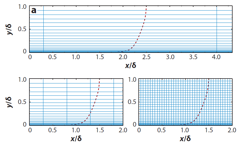
If we assume that the x-direction runs along the wall-parallel direction (from left to right) and the y-direction in the wall-normal direction (from bottom to top), then we can say that \Delta_x \gg \Delta_y, and therefore \Delta \gt \delta, where \delta is the height of the boundary layer (we can see that the y-axis is normalised by the boundary layer height so we get a sense for how large the boundary layer is in this case).

If \Delta \gt \delta, this means that within the boundary layer, according to Eq.(56), we will always pick the RANS-based length scale l^{RANS} and thus produce sufficient turbulent viscosity to damp fluctuations.

If we look at the grid on the bottom right, then we have a very fine resolution, where we have \Delta_x \approx \Delta_y. In this case, we have \Delta \lt \delta and so we use an LES description in the entire boundary layer. This is one particular nice feature of DES, that it switches between RANS and LES depending on the grid resolution.

Amazing, we have unified RANS and LES and depending on the grid, our solver will automatically switch between the right definition, right? The issue comes in when we are just at the border between RANS and LES resolution in terms of the grid size. This is shown in the figure above with the bottom left grid.

Here, \Delta is smaller than the boundary layer height \delta, so this isn’t a clear RANS region, though the size of \Delta is too large to effectively capture turbulence through an LES description. Thus, if we were to use LES, we would not resolve the turbulent stresses sufficiently to get an accurate reading on the subgrid-scale stresses, but \Delta is computed to be sufficiently small so that it blocks RANS from kicking in.

Spalart refers to this phenomenon as modelled-stress depletion (MSD), and the consequences of MSD are rather significant. Take a look at the flow around an airfoil, which is shown below:

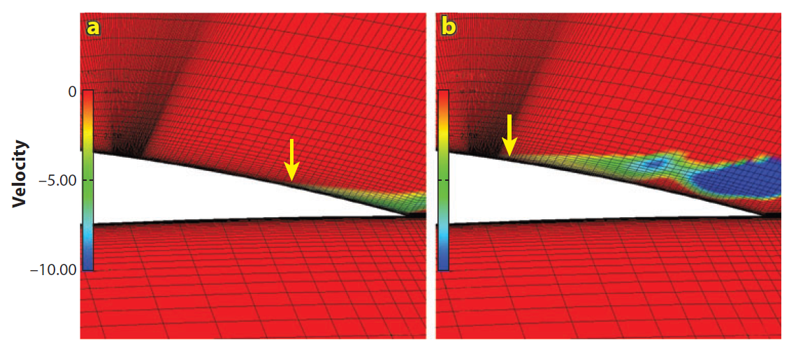
On the left-hand side, we see numerical results that match experimental observations in terms of flow separation. The point at which the flow separates is shown by the yellow arrow. On the right-hand side, we see results obtained with the standard DES formulation. The grid was arbitrarily refined upstream of the expected separation point, and we see that at the point where the grid is refined, separation occurs. As a result, this process is known as grid-induced separation, or GIS.

Delayed detached eddy simulation (DDES) overcomes this problem by redefining the length scale computation. In standard DES, we had:

l^{DES}=\min[d, C_{DES}\Delta]\tag{64}

I have inserted the length scale definitions and changed the closure coefficient from C_{LES} to C_{DES}. So how does that change in DDES? Well, for starters, we no longer just compare two length scales and pick whichever is smallest, but instead, we incorporate some information about the local flow into the computation, so that we can distinguish between wall-bounded (boundary layer) flows and those far away from it.

The length-scale for DDES is computed as:

l^{DDES} = l^{RANS} - f_d \max[0, l^{RANS}-l^{DES}]
\tag{65}

Here we have introduced a so-called shielding function f_d, which we want to be zero close to the wall, regardless of the grid spacing, and close to one in the outer part of the boundary layer and farfield. In this way, we have a smooth blend between RANS and LES in terms of the length scale computation.

So let’s inspect f_d, it is given by:

f_d = 1 -\tanh\left[\left(C_{f_d} r_d\right)^3\right]\tag{66}

The value for C_{f_d} is set to 8, and one must wonder if the subscripts were chosen by accident or if Spalart was just having a bit of fun. CFD-engineering humour, I suppose. Regardless of the value of r_d, given that we are using the hyperbolic tangent function here, which is clamped between -1 and 1, the value of f_d is between 0 and 1 and only depends on the value of r_d. This function, in turn, is defined by:

r_d = \frac{\nu + \nu_t}{(\kappa d)^2\max[S_{mag}, 10^{-10}]}
\tag{67}

Let’s look at the denominator and see what happens near the solid wall and away from it. At solid walls, the value for d will be small and close to zero. Squaring it will make it even smaller. S_{mag}, the magnitude of the shear-stress tensor (collection of mean flow velocity gradients), is generally non-zero for attached flows but may locally become zero in regions where the flow separates.

Taking the max value here of the magnitude of the shear stress tensor and a small number (the exact value is really rather inconsequential) will ensure that we are not dividing by zero. If the shear stress tensor magnitude does become zero, the max expression will evaluate to 10^{-10}. Dividing \nu+\nu_t by this magnitude will result in a large value, but it doesn’t matter what the magnitude here is, as the result is piped through the hyperbolic tangent function.

For the sake of argument, a value of 10 and 100 will return pretty much the same value when put into the hyperbolic tangent function. We get \tanh(10)=0.999999996 and \tanh{100}=1.00000000. Larger values will not change the result, and we will essentially get 1 returned from the hyperbolic tangent.

As we get away from the wall, d will grow and S_{mag} will have some finite value. In general, the equation for r_d has been calibrated so that towards the outer edge of the turbulent boundary layer, we get a value of close to zero. The hyperbolic tangent function at zero is zero itself, and so the shielding function becomes f_d=1 towards the outer edge of the turbulent boundary layer.

With the shielding function being one, we allow for l^{DES} to influence the computation of l^{DDES} in Eq.(65). In this way, we avoid grid-induced separation close to solid walls with a gradual transition towards LES-like resolution in the farfield and away from turbulent boundary layer flows.

Returning back to the example of the flow over an airfoil, the figure we saw above used DDES on the left and DES on the right. We see that despite local grid refinement, DDES is successfully able to predict the correct flow behaviour, matching experimental results, showing a clear improvement over the standard DES formulation.

Since the only difference between DES and DDES is the improved length scale computation, there is no reason not to use DDES. The only time you probably want to use DES is when you want to showcase the phenomenon of grid-induced separation. Otherwise, there is no benefit in using DES, but you gain additional uncertainty over your grid, which can’t be quantified with, for example, a grid dependency study.

Improved Delayed Detached-eddy simulations (IDDES)

OK, I just said that DDES should be seen as the new standard DES. It removes grid-induced separation, so what else could we want? Well, DDES made hybrid RANS-LES even more popular, given that early identified issues were fixed quickly, drawing in even more people to play around with (D)DES. More users mean that even more issues may be unearthed, and it wasn’t long before people used DDES for wall-bounded flows and assessed its capabilities against classical academic benchmark cases.

One of the most fundamental test cases we can think of, in terms of turbulence modelling, is the flow with a zero pressure gradient past a flat plate. It is so fundamental and important that you will see this in any turbulence lecture at university (I certainly bring it up a few times in my lectures!). Here, the flow is developing first a laminar boundary layer, which then transitions to a turbulent one.

We have a well-established theory for flat plate flows and there are a few concepts we can take from this theory to test that our CFD solver is reproducing certain key characteristics. One of the most fundamental characteristics is the velocity profile, and, in fact, it is so important that it has its own name; the law of the wall. If this is new to you, then you may want to check out my write-up on turbulent boundary layers, which covers the law of the wall.

Suffice it to say that the law of the wall is a universal description of velocity profiles in turbulent boundary layers. Both the x and y axes are non-dimensionalised, and any turbulent boundary velocity profile will collapse onto the law of the wall. This makes it an ideal test ground for checking if a turbulence model matches the expected behaviour within the boundary layer.

And so, people unleashed (D)DES and applied it to such flow scenarios, and the results for a few different test conditions are shown in the following picture, where a comparison between RANS (Spalart-Allmaras), DES, DDES, and IDDES is made:

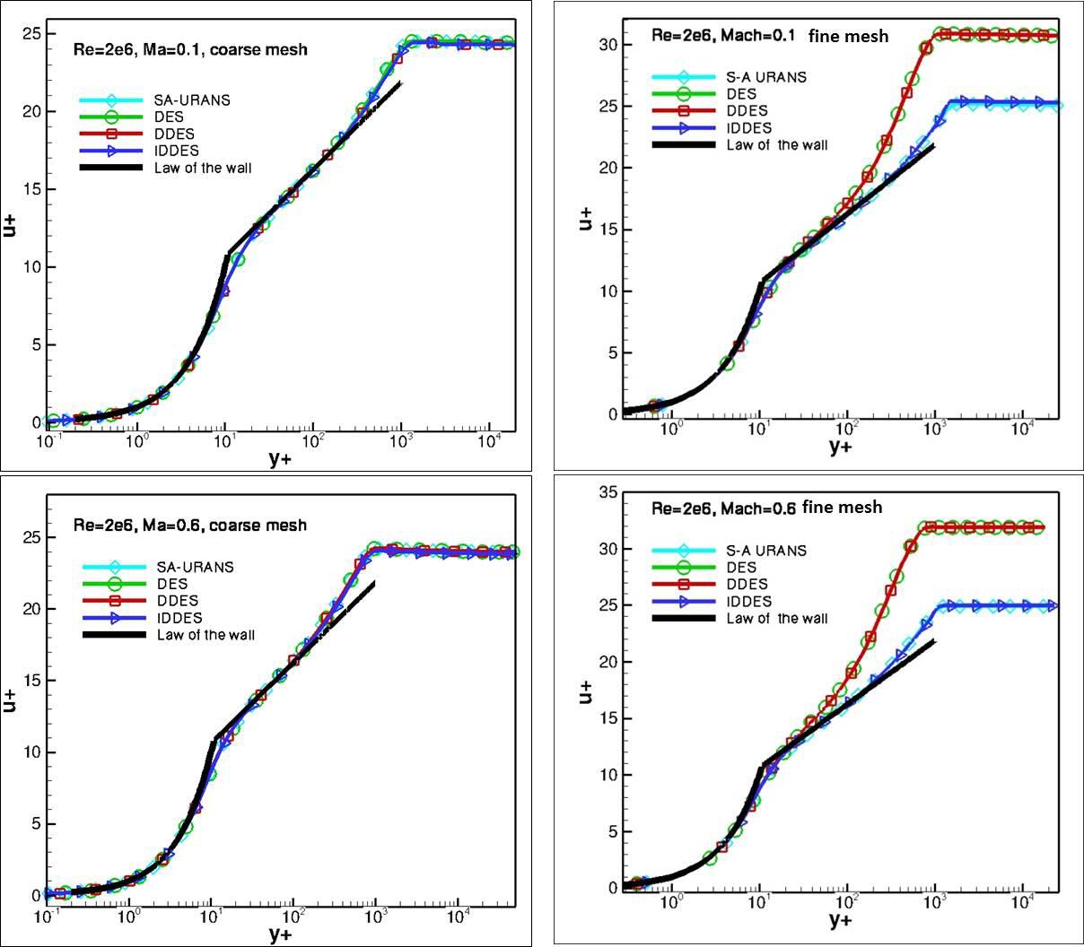
As we can see, only IDDES is capable of matching the law of the wall in all regions of the turbulent boundary layer. So what is this magical IDDES and why was it introduced?

First things first, IDDES stands for Improved Delayed Detached Eddy Simulations. Lovely name! I wouldn’t be surprised if the next incarnation will be called something like LIDDES (Latest IDDES) or MIDDES (Matured IDDES). BORING! Why do that when HYDDIES is on the table? We just need 2 more letters to get there. Why not!? (I also had to rearrange the I, but don’t tell anyone!)

It is settled, if you read this article and work on IDDES, and you are improving it through a new length scale definition or something, then you are morally obliged to name your model HYDDIES. I’ll let you decide what the letters H and Y should stand for (and why the I needs to be moved!), but please don’t add boringness like HYbrid, aim for a standard like Holistic Yielding, which sounds just as ridiculous as any of the other letters in IDDES.

I think the people who came up with DES, DDES, IDDES, and the like are the same people whose idea of version control is to name your files NEW000000.F, NEW000001.F, new_000002.F, and so on (yes, of course, a break in naming style is mandatory). How did we get this much off-topic again?

IDDES was specifically introduced to tackle this mismatch in the law of the wall, which is known as the logarithmic layer mismatch (as deviations are introduced in the logarithmic layer of the turbulent boundary layer). Let’s go back, once more, to the length scale calculation of our standard DES approach. This was given as:

l^{DES}=\min[d, C_{DES}\Delta]\tag{68}

On the surface, this equation may appear innocent, but there is one big problem with this type of description. It introduces a discontinuity. Somewhere in the boundary layer, we will switch from RANS resolution to LES resolution, and this will result in a different length scale. Thus, at the interface between RANS and LES, the length scale will be discontinuous. Since the length scale is used to compute the dissipation, this will be discontinuous, and there will be a sudden change in production/destruction terms in the turbulence equations.

This ultimately results in the behaviour that we see in the previous figure, where both DES but crucially also DDES start to deviate from the law of the wall. This deviation starts where we switch from RANS to LES. If this switch appears closer to the edge of the boundary layer, then the law of the wall will be mostly matched, but if it happens closer to the beginning of the logarithmic layer, then we get into trouble. Where we will switch from RANS to LES is entirely driven by the mesh and local flow properties and thus difficult to control.

So, IDDES tries to avoid this logarithmic layer mismatch and, as we have already seen, is rather successful at it. So let’s look at how this can be achieved. The length scale in IDDES is computed as:

l^{IDDES}=f_\beta (1+f_e)l^{RANS} +(1-f_\beta)l^{DES}
\tag{69}

There are two additional functions given here, of which f_\beta is computed as:

f_\beta = \min[2 \exp(-9\alpha^2), 1]\\[1em]
\alpha = 0.25 - \frac{d}{\max(\Delta_x, \Delta_y, \Delta_z)}\tag{70}

We can see that f_\beta is limited to values between 0 and 1. Thus, in Eq.(69), if we ignore the value for f_e for the moment, then we can say that the length scale l^{IDDES} is a smooth blend between the RANS and LES length scale. Introducing this smooth blending removes any discontinuities at the interface of the RANS and LES regions.

The crucial part in IDDES is how we define the f_e function, which is responsible for removing the logarithmic layer mismatch. It is given as:

f_e = \max[f_{e1} - 1, 0] f_{e2}
\tag{71}

Here, the additional functions f_{e1} and f_{e2} are given as:

f_{e1} =
\begin{cases}
2\exp(-11.09 \alpha^2) &\alpha \ge 0 \\[1em]
2\exp(-9.0\alpha^2) & \alpha \lt 0
\end{cases}\tag{72}

and

f_{e2} = 1 - \max\left[\tanh\left\{(c_t^2r_{d_t})^3\right\}, \tanh\left\{(c_l^2r_{d_l})^10\right\}\right]\tag{73}

Let’s look at f_{e1}. This depends on the value of \alpha, which in turn depends on the value of d/\max(\Delta_x, \Delta_y, \Delta_z). This is, in essence, the length scale ratio between RANS and LES (just the closure coefficient C_{LES} or D_{DES} is missing). If this ratio is 0.25, i.e. the LES length scale is 4 times larger than the RANS length scale, then \alpha=0 and f_{e1} = 1. As we move away from this, f_{e1} reduces regardless of which direction we go (i.e. increasing or decreasing \alpha).

If we insert f_{e1} now into Eq.(71), we see that we take the maximum value between f_{e1} and 0. Once f_{e1} becomes negative, we clip this value to zero. Thus, at \alpha=0, we have a maximum of f_{e1}=1 and this then reduces to zero. We can see that this function is only switched on in a region where we expect the cross-over between RANS and LES to happen. Crucially, this is not a hard switch from one region to another, but rather a smooth blend, which is indicated by the exponential function (\exp()).

Thus, the purpose of f_{e1} is to detect where the cross-ver is happening. The magnitude of f_e, as seen in Eq.(71), is calculated based on f_{e2}. This function, in turn, uses our friend the hyperbolic tangent function, which will ensure again that we get values of 0 when the argument to the hyperbolic tangent is zero itself, and +1 or -1 for values in the positive or negative direction.

The values r_{d_t} and r_{d_l} are the turbulent and laminar portion of r_d, as introduced in Eq.(67). The values of c_t and c_l are just additional closure coefficients. Therefore, the range of f_{e2} is between 0 and 2, and we can see this function as an amplification to f_{e}.

If we look at Eq.(69) again, we see that (1 + f_e) is multiplied by the RANS length scale. Thus, in regions where we are purely within RANS or LES, f_{e1} will be zero and so f_e will be zero, too. But, near the cross-over between RANS and LES, f_{e1} becomes non-zero and it is scaled by f_{e2} which depends on r_d (Eq.(67)), and this in turn depends on the turbulent viscosity and the magnitude of the shear stress tensor.

Therefore, we simply give more weight to the RANS length scale by multiplying it with (1 + f_e). This simple multiplication will ensure that we do not suddenly lose too much dissipation by switching from RANS (dissipative) to LES (less dissipative) too quickly. The closure coefficients c_t and c_l are then tuned in a way that the velocity profile (law of the wall) within the boundary layer matches the expected behaviour.

In the previous section, I said that DDES should be regarded as the new DES. In this section, I am saying that really, you may as well just go for IDDES instead, as you are, again, not losing anything, and the increase in computational cost is laughable.

There is one more thing, though. IDDES has been designed to give DDES resolution in the worst case (coarse grid) and WMLES resolution in the best case (fine grid). What is WMLES? Well, we are getting ahead of ourselves; we first have to cover a closely related concept to I/D/DES, which is called Scale Adaptive Simulations (SAS). Let’s do that first, and then we’ll return to WMLES after that. TL;DR: It is an improved description over DES and resolves more physical flow features and thus is, potentially, more accurate, albeit more expensive to run.

Scale adaptive simulations (SAS)

It is the year 2003. The Columbia space shuttle breaks up during re-entry, the war in Iraq started, a heat wave reaches Europe recording 38 degree Celcius (100 degree Farneheit) and claimed 35,000 lives (fast forward 20 years and air conditioning is still not common in Europe), a blackout left 50 millions Americans without electricity, the concord made its final flight and the third entry in the Lord of the Rings trilogy was released.

But it was not all bad, Schwarzenegger became the governor of California and showed that reality TV stars belong in public office (great), the last Volkswagen Beetle was produced in Mexico, and Britney Spears and Madonna kissed at the VMA. Since most of my readers will be students in their 20s, they will have no idea who Brittney Spears or Madonna are, what the VMA is, and this makes me feel very old. That is alright.

At the same time, Menter, in many ways the spiritual successor of Prandtl when it comes to turbulence research Made in Germany (reading this wikipedia entry is hilarious, German-Britsh friendship at its finest), was quietly deriving away equations on 80 g/m^2 A4 paper (a wild assumption on my behalf, perhaps Menter has a much more complex personality and prefers 100 g/m^2. That is something the historians will have to answer once and for all (I know he is still alive, but it would be weird to ask him …)).

Menter was looking for a way to give URANS a less dissipative character so that it can be used to resolve physical phenomena not captured by steady-state RANS at the cost of URANS and not LES. Conceptually, Menter’s new framework, which he would call Scale-Adaptive Simulations (SAS), was very closely aligned with Spalart’s DES approach, yet different in key characteristics.

The underlying idea of SAS is very similar to DES: Reformulate the length scale found in RANS equations to give a better approximation of the dissipation away from the wall. In DES, we said that we take the minimum of either the RANS or LES lengthscale. In the case of the Spalart-Allmaras model, we saw that the RANS length scale was just the distance from the wall.

Menter postulated that we should use a physical length scale instead, and not rely on either the distance from the wall (Spalart-Allmaras model), k and \varepsilon or \omega to compute a length scale (two equation RANS model), or the grid spacing (LES). He settled on the von Karman length scale, which for a flat plate flow is given as:

l^{vk} = \left|\frac{\partial u / \partial y}{\partial^2 u / \partial y^2}\right|
\tag{74}

Let’s get some idea about what this equation is doing. For this, let us look at the law of the wall again. For convenience, this is reproduced below:

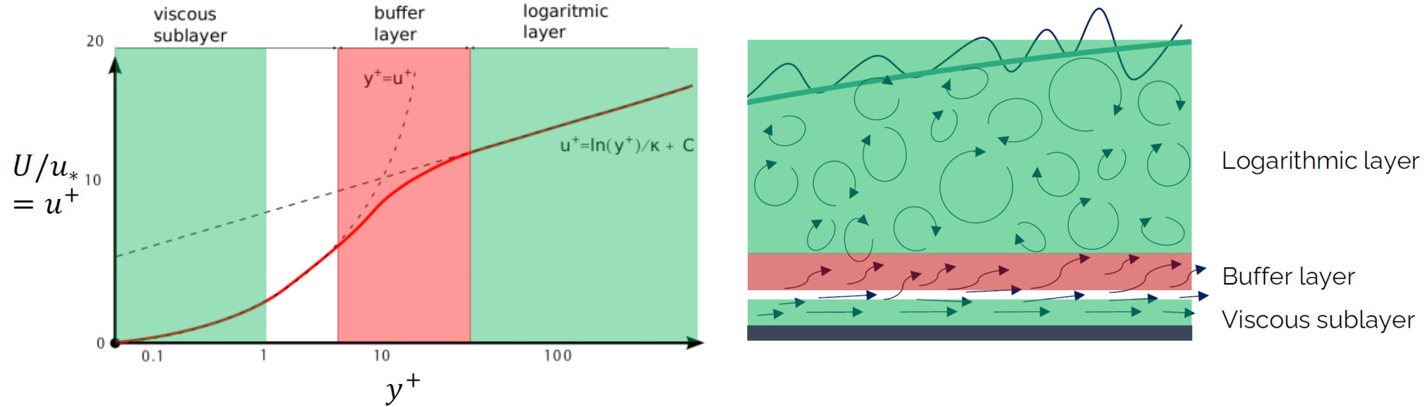
In the logarithmic layer, we can see that the non-dimensional velocity profile for u^+ is given as:

u^+ = \frac{1}{\kappa}\ln\left(\frac{u_\tau y}{\nu}\right) + B\tag{75}

Here, y^+ = u_\tau y / \nu, so the non-dimensional velocity profile is both non-dimensional in terms of its velocity and wall-normal distance y (i.e. y^+). We can expand this equation now as:

u^+ = \frac{1}{\kappa}\ln\left(u_\tau\right) + \frac{1}{\kappa}\ln\left(y\right) - \frac{1}{\kappa}\ln\left(\nu\right) + B
\tag{76}

Taking the first derivative of Eq.(76) with respect to y, noting that \mathrm{d}\ln(x) / \mathrm{d}x = 1/x, we obtain:

\frac{\mathrm{d}}{\mathrm{d}y}u^+ = \frac{\mathrm{d}}{\mathrm{d}y}\frac{1}{\kappa}\ln\left(u_\tau\right) + \frac{\mathrm{d}}{\mathrm{d}y}\frac{1}{\kappa}\ln\left(y\right) - \frac{\mathrm{d}}{\mathrm{d}y}\frac{1}{\kappa}\ln\left(\nu\right) + \frac{\mathrm{d}}{\mathrm{d}y}B = \\[1em]
0 + \frac{1}{\kappa y} - 0 + 0 = \frac{1}{\kappa y}
\tag{77}

Taking the derivative of Eq.(77) results in the second derivative, i.e.:

\frac{\mathrm{d^2}}{\mathrm{d}y^2}u^+ = \frac{\mathrm{d}}{\mathrm{d}y}\frac{1}{\kappa y} = -\frac{1}{\kappa y^2}
\tag{78}

Now we can insert these two definitions into Eq.(74) to get an idea for what the von Karman length scale is:

l^{vk} = \left|\frac{\frac{1}{\kappa y}}{-\frac{1}{\kappa y^2}}\right| = y\tag{79}

Since we are currently considering the flow past a flat plate, where the wall normal direction is in the y direction, we can see that the length scale in this case reduces to just the distance away from the wall, which is the same length scale as used by the Spalart-Allmaras model, i.e. l^{RANS}=d.

Now you might be asking, what’s the point then? If the length scale is identical, why bother? Well, this derivation is only applicable for the logarithmic layer. Away from the wall, the velocity gradients will be affected by the boundary conditions and local geometry. Thus, based on the local flow properties, we have an adaptive way of determining the local length scale. Contrast that with l^{RANS}=d from the Spalart-Allmaras model; this will simply increase in size away from the wall.

Now what about two-equation models? They compute their length scale based on k and \varepsilon or \omega. Yes, that is true, but as Menter shows in his papers, the length scale that is obtained in this way is overly dissipative. For RANS, this is a good thing, as it can dampen fluctuations that we don’t want to arise (after all, we want to drive the solution to a steady state). But, once we go for unsteady RANS, we do want the physical fluctuations to develop, and this requires a less dissipative approach.

Menter’s hope was that by providing a physically inspired way to compute a local length scale, rather than relying on the RANS or LES length scale, a scale-adaptive formulation could be derived that would locally resolve more physical unsteadiness and fluctuations if run as an unsteady RANS (URANS) model.

Thus, in order to achieve that, we need to replace the length scale in our RANS equations. For the Spalart-Allmaras turbulence model, for example, replacing d=l^{vk} results in:

\frac{\partial \tilde{\nu}}{\partial t} + (\mathbf{u}\cdot\nabla)\tilde{\nu} = \frac{1}{\sigma}\nabla\cdot[(\nu+\tilde{\nu})\nabla\tilde{\nu}] + \frac{c_{b2}}{\sigma}\nabla\tilde{\nu}\cdot\nabla\tilde{\nu} + c_{b1}(1-f_{t2})\tilde{S}\tilde{\nu} + f_{f2}\frac{c_{b1}}{\kappa^2}\left(\frac{\tilde{\nu}}{l^{vk}}\right)^2-c_{w1}f_w\left(\frac{\tilde{\nu}}{l^{vk}}\right)^2
\tag{80}

In the k-\omega SST model, the governing equation for the turbulent kinetic energy was given in Eq.(57), which is repeated below for convenience:

\frac{\partial k}{\partial t} + (\mathbf{u}\cdot\nabla)k = \nabla\cdot\left[\left(\nu+\sigma^*\nu_t\right)\nabla k\right] + P - \beta^* k\omega\tag{81}

We saw that the length scale definition was hidden in the last term, which could also be formulated as:

\beta^* k\omega = \beta^*\frac{^{\frac{3}{2}}}{l^{RANS}}\tag{82}

In this equation, we simply set l^{RANS}=l^{vk} and obtain:

\beta^* k\omega = \beta^*\frac{^{\frac{3}{2}}}{l^{vk}}\tag{83}

This is Menter’s (and his co-workers’) Scale-Adaptive Simulation (SAS) framework applied to the Spalart-Allmaras and k-\omega SST RANS equations.

We could leave it there, but Menter went one step further and also introduced a hybrid RANS-LES version of the SAS framework. In it, the length scale is computed as:

l^{SAS}=\max[l^{vk}, C_{SAS}\Delta]
\tag{84}

Contrast that with the original DES length scale formulation:

l^{DES}=\min[d, C_{DES}\Delta]\tag{85}

There is one big difference here: DES uses a \min() operator, while SAS uses a \max() operator. In DES, this means that LES-like resolution may be achieved close to the wall and that the LES length scale may be used, even if the mesh is too coarse. This led to modelled-stress depletion (MSD), which manifested itself through grid-induced separation (GIS).

In SAS, this cannot occur because we take the maximum of the two length scales. Menter was able to show that this avoids GIS; however, SAS remains a much less frequently used turbulence formulation compared to DES.

However, as we can see, DES and SAS share many similarities, i.e. in both descriptions, the length scale computation is changed. This then leads to a modified RANS equation that allows for both RANS-like and LES-like resolution, as long as the grid is fine enough and the hybrid length scale computation is used in SAS.

Thus, if you are writing your own code and you are implementing DES, you may as well throw it in SAS for good measure; it really doesn’t cost you that much more mental effort to get it implemented.

But let’s turn to the big daddy of them all; Wall-Modelled Large Eddy Simulations, or WMLES, in short. We’ll look at it in the next section.

Wall-modelled Large Eddy Simulations (WMLES)

In wall-modelled LES (WMLES), we don’t model the wall. We are off to a great start! No, it is not the wall that is modelled, but rather, the flow near the wall. So, if we want to be pedantic (and I am feeling particularly pedantic today on this hot July summer day), we ought to call it Near-wall modelled LES, or NWMLES, but that acronym just doesn’t roll off the tongue, so I suppose we have to stick with the WMLES nomencalture.

Be that as it may, WMLES is, in many ways, very similar to DES and co., and we can say that it is a kind of hybrid RANS/LES model. The main difference between DES/SAS and WMLES is the grid resolution requirement (we need more cells for WMLES and therefore hope to get a better prediction of turbulent boundary layers) and how the near-wall modelling is introduced into LES.

For SAS and DES (and its derivatives), we started with the RANS equations and then introduced LES-like resolution by modifying the local turbulence length scale. in WMLES, we start with the LES equations and then introduce RANS or an algebraic model near the wall to model the near-wall flow. Let’s look at two schematic figures to show WMLES in action. The first figure is shown below:

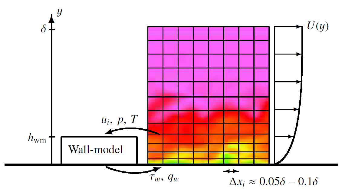
Here, we see the flow past a flat wall (plate), which forms a turbulent velocity profile U(y), as seen on the right. On the left-hand side, we see the wall-normal coordinate direction extending from the wall. Along this line, we have an arbitrarily chosen value h_{wm}, which indicates some height above the wall. The value for h_{wm} is typically set to be somewhere close to the start of the logarithmic layer of the boundary layer, i.e. a y^+ of around 30-50 (this value may vary from case to case but is just given as a rule of thumb).

At this height above the solid wall, we sample flow properties such as the velocity and pressure, but also temperature if we solve for the energy equation. We put these properties into our wall-model (which we will look at in more detail later), and it will give us properties that we can use to impose at the solid wall itself, typically the wall shear stresses, but also the heat flux, in case of temperature-dependent simulations.

So what is the benefit of this approach? Well, by sampling flow properties away from the wall, and then using these to compute boundary conditions, like the wall shear stresses, at the wall, this means that we no longer need the flow field information near the wall. Thus, everything below h_{wm} is essentially a modelled behaviour, and the wall model is what gives WMLES its name.

In practice, this means that we do not have to apply the same grid spacing near the wall compared to traditional LES. The hope is that the wall model will give us results at the wall that are indistinguishable from pure LES simulations, and using these boundary conditions, we can get a realistic flowfield near the wall, without resolving the near field flow explicitly. If that is given, then the grid requirements for WMLES become far less compared to LES, making it suitable for engineering and high Reynolds number applications.

The second approach of WMLES is given below:

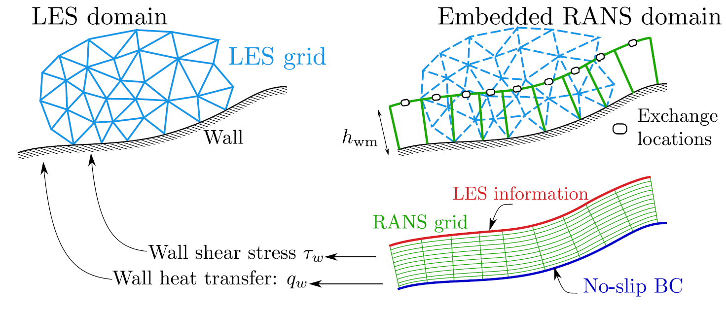
Here, we have our normal grid, as shown in the top left, and then we decide on some sampling height for h_{wm} again, which is seen on the top right. We then extract this height above the wall and insert a mesh from the solid boundary all the way to this newly extracted line, which is shown on the bottom right.

We then go on to solve some form of RANS equations on this new, secondary grid, where the boundary conditions at the top (red line) are taken directly from the LES domain. We then solve the flow and obtain the velocity profile on this grid, from which the wall shear stresses can be obtained. Once these stresses are available, we can impose them back on our LES domain (top left part of the figure), and these will drive the flow development near the wall again.

We typically use a RANS model here on the second grid, though other approaches have been proposed and tested in the literature. You might be asking yourself: Why do we need to go through all that trouble? Wouldn’t it be just easier to use LES instead of having to construct a secondary grid? Well, yes and no.

It would be either to use LES throughout the entire domain, but it would be too expensive in terms of computational cost, especially for high Reynolds number engineering applications. Instead, using a RANS model in the near-wall region, we can construct a relatively coarse mesh (compared to LES) and get away with much larger cells, reducing the computational cost as a result. The same argumentation holds for the first figure above, i.e. our goal is always to reduce computational cost by not resolving the flow in the near-wall region.

I have mentioned the wall shear stresses \tau_w now a few times, so let’s explore why this property is of particular interest in WMLES. For that, let us return back to the governing momentum equation for LES. This was given as:

\underbrace{\frac{\partial \bar{\mathbf{u}}}{\partial t}}_\text{Term 1} + \underbrace{(\bar{\mathbf{u}}\cdot\nabla)\bar{\mathbf{u}}}_\text{Term 2} = -\underbrace{\frac{1}{\rho}\nabla\bar{p}}_\text{Term 3} + \underbrace{\nu\nabla^2 \bar{\mathbf{u}} + \nabla\cdot\tau^{SGS}}_\text{Term 4}
\tag{86}

Here, \tau^{SGS} are the subgrid scale stresses that result from the spatial filtering process of the momentum equations. Let’s consider how this equation is evaluated near the wall. For this, consider the following simple, structured grid:

Here, I have shown two locations in particular; p_w is the location at the wall for the bottom left cell, while its centroid is given by p_c. Let’s return to the LES momentum equation and see which of these terms will be active at the wall.

Since the velocity has a no-slip boundary condition, meaning that it will have the same velocity at the wall (and, if the wall is not moving, this means that the velocity is zero at the wall), we have not changes in velocity over time at p_w. Therefore, the time derivative (Term 1 in Eq.(86)) is zero. The convective term (Term 2) will be zero as well due to the no-slip condition.

The pressure gradient term (Term 3) is not zero. At solid walls, the pressure is considered to be constant in the wall normal direction. Therefore, we can simply assume the value of the pressure at p_w to be equivalent to the value of the pressure at p_c. This is exactly what a Neumann-type boundary condition will achieve, i.e. it will simply copy information from the interior domain onto the boundary. We have looked at this in depth in my article on boundary conditions.

So, the value of the pressure at the wall is non-zero, but we can easily obtain it. Now let’s look at Term 4 in Eq.(86). First, let us re-express it in a different notation:

\tau_w = \nu\nabla^2 \bar{\mathbf{u}} + \nabla\cdot\tau^{SGS} = \nabla\left(\nu\nabla \bar{\mathbf{u}} + \tau^{SGS}\right)\tag{87}

\tau_w represents the wall shear stresses and while we can compute the first term (the diffusion operator), we can’t compute the second term, i.e. the subgrid scale stresses. Why? In LES, we saw that this term arises as we make our computational grid too coarse to resolve all turbulent eddies. The subgrid scale model assumes that most the turbulent kinetic energy (the largest eddies) is resolved, and therefore it only needs to account for the viscous dissipation at the smallest scales.

In WMLES, we are now reducing the mesh size drastically (increasing the cells near the wall), and we potentially no longer resolve even the largest eddies. Thus, our subgrid scale model would not just need to account for viscous dissipation at the smallest scales but also physical processes along the entire turbulent kinetic energy spectra. Thus, we can’t simply use a subgrid scale model for \tau^{SGS} but instead try to model the wall shear stresses completely, i.e. \tau_w.

As we have seen above, the idea is to sample the LES flowfield at some distance h_{wm} away from the wall, and use that information to compute the wall shear stresses. Thus, the role of the wall model is to compute the value of the wall shear stresses at the boundaries. This wall shear stress will then be used within the LES simulation to obtain realistic near-wall behaviour within turbulent boundary layers. Let’s look at three common and popular choices for obtaining \tau_w.

Logarithmic profile

Our goal in wall-modelled LES is to model the near-wall region. As we have seen, this typically results in cell sizes that are larger than the viscous sublayer, as well as the transition region in the law of the wall, and our first cell height reaches into the logarithmic layer. This means that, in terms of non-dimensional y^+ units, our first cell height is in the region of y^+>30.

In that case, we know what the velocity profile is from the law of the wall. For the logarithmic portion, the velocity profile is given as:

u^+ = \frac{1}{\kappa} \ln\left( \frac{y u_\tau}{\nu} \right) + B
\tag{88}

Here, u^+ is the non-dimensional velocity given as:

u^+ = \frac{u}{u_\tau} \quad \rightarrow \quad u_\tau = \frac{u}{u^+}
\tag{89}

y^+ = y u_\tau / \nu is the non-dimensional wall normal coordinate, which appears in the logarithm. \kappa \approx 0.41 is the von Karma constant, which you will often find in the turbulence literature, and B \approx 5.2 is found from measurements (the intersection of u^+ with the y-axis, i.e. when y=0). Using Eq.(88) and Eq.(89), we can compute the wall shear stresses \tau_w from the definition of the friction velocity u_\tau as:

u_tau = \sqrt{\frac{\tau_w}{\rho}} \quad \rightarrow \quad \tau_w = \rho u_\tau^2
\tag{90}

There is just one problem. We want to obtain \tau_w, which in turn is obtained from u_\tau. But, let’s insert Eq.(89) into Eq.(88), this results in:

\frac{u}{u_\tau} = \frac{1}{\kappa} \ln\left( \frac{y u_\tau}{\nu} \right) + B
\tag{91}

Now we have u_\tau both on the left-hand and right-hand side of the equation, and since it appears within the logarithmic expression, we can’t solve for u_\tau. This means that we have to find a value for it numerically. Whenever we have to find a value approximately and we have a (differentiable) function available, we can use a numerical procedure like the Newton-Rhapson method. This is given as:

u_\tau^{n+1} = u_\tau^n - \frac{f(u_\tau^n)}{f'(u_\tau^n)}
\tag{92}

Let’s look at each term. We want to solve for u_\tau^{n+1}, which is the value we obtain after completing the n-th iteration. The value of u_\tau^n is either the value for the friction velocity from the previous iteration, or an initial guess if we are just starting with the procedure.

Then we have two functions, the first is the functional relation for u_\tau itself (f(u_\tau)), while the second is the derivative of this function (f'(u_\tau)). The function itself can be obtained from Eq.(91), which becomes:

f(u_\tau) = \frac{u}{u_\tau} - \frac{1}{\kappa} \ln\left( \frac{y u_\tau}{\nu} \right) - B\tag{93}

Here, we simply brought all terms onto one side (meaning that one side becomes zero), and then we call the remaining non-zero side f(u_\tau). Let us expand the second term first, before we attempt to construct its first derivative. This results in:

f(u_\tau) = \frac{u}{u_\tau} - \frac{1}{\kappa} \ln(y) + \frac{1}{\kappa} \ln(u_\tau) - \frac{1}{\kappa} \ln(\nu) - B
\tag{94}

Let us now differentiate Eq.(94) with respect to u_\tau. We get:

\frac{\text{d}f(u_\tau)}{\text{d}u_\tau}=f'(u_\tau)= -\frac{u}{u_\tau^2} - 0 + \frac{1}{\kappa u_\tau}
\tag{95}

Using Eq.(94) and Eq.(95) in Eq.(92), we can now iteratively compute a solution for u_\tau, and then use Eq.(90) to compute the wall-shear stresses \tau_w from u_\tau. An example implementation of this is given in the Python code below, where the iteration is stopped when the difference between u_\tau^{n+1} and u_\tau^n is less than 10^{-8}. Parameters for the turbulent boundary layer are arbitrarily set and would come from the CFD solution.

from math import log, pow

def f_u_tau(u, y, nu, u_tau):
  return ((u / u_tau) - (1 / 0.41) * log(y * u_tau / nu) - 5.2)
  
def df_u_tau(u, u_tau):
  return (-u / pow(u_tau, 2)) - (1 / (0.41 * u_tau))
  
def newton_rhapson(u, y, nu, u_tau, max_iterations, tolerance):
  for i in range(1, max_iterations):
    f_val = f_u_tau(u, y, nu, u_tau)
    df_val = df_u_tau(u, u_tau)
    u_tau_new = u_tau - f_val/df_val
    if abs(u_tau_new - u_tau) < tolerance:
      break
    u_tau = u_tau_new

  print(f"Converged u_tau = {u_tau:.6f} after {i} iterations")
  print(f"Computed  y+    = {(y * u_tau / nu):.1f}")
  
# turbulent boundary layer parameters
u = [0.05, 0.2, 1.0]
y = 1e-3
nu = 1e-6

# initial value for u_tau, can be anything
u_tau = 0.01

# newton-rhapson iteration
max_iterations = 100
tolerance = 1e-8

# calculate u_tau using Newton-Rhapson method
for u_value in u:
  newton_rhapson(u_value, y, nu, u_tau, max_iterations, tolerance)

from math import log, pow

def f_u_tau(u, y, nu, u_tau):
  return ((u / u_tau) - (1 / 0.41) * log(y * u_tau / nu) - 5.2)
  
def df_u_tau(u, u_tau):
  return (-u / pow(u_tau, 2)) - (1 / (0.41 * u_tau))
  
def newton_rhapson(u, y, nu, u_tau, max_iterations, tolerance):
  for i in range(1, max_iterations):
    f_val = f_u_tau(u, y, nu, u_tau)
    df_val = df_u_tau(u, u_tau)
    u_tau_new = u_tau - f_val/df_val
    if abs(u_tau_new - u_tau) < tolerance:
      break
    u_tau = u_tau_new

  print(f"Converged u_tau = {u_tau:.6f} after {i} iterations")
  print(f"Computed  y+    = {(y * u_tau / nu):.1f}")
  
# turbulent boundary layer parameters
u = [0.05, 0.2, 1.0]
y = 1e-3
nu = 1e-6

# initial value for u_tau, can be anything
u_tau = 0.01

# newton-rhapson iteration
max_iterations = 100
tolerance = 1e-8

# calculate u_tau using Newton-Rhapson method
for u_value in u:
  newton_rhapson(u_value, y, nu, u_tau, max_iterations, tolerance)

The output that will be printed is:

Converged u_tau = 0.007363 after 26 iterations
Computed  y+    = 7.4
Converged u_tau = 0.018126 after 28 iterations
Computed  y+    = 18.1
Converged u_tau = 0.065910 after 30 iterations
Computed  y+    = 65.9

Converged u_tau = 0.007363 after 26 iterations
Computed  y+    = 7.4
Converged u_tau = 0.018126 after 28 iterations
Computed  y+    = 18.1
Converged u_tau = 0.065910 after 30 iterations
Computed  y+    = 65.9

Spalding wall function

The aforementioned velocity profile from the logarithmic layer is typically chosen. But there is one limitation: it assumes that we are indeed in the logarithmic layer. If our flow locally drops into the transition or even the viscous sublayer, the wall shear stresses we obtain from our logarithmic layer will be inadequate.

You might argue that this isn’t really a problem, as the whole point of WMLES is to model the near-wall flow, and thus we aim to always have our first cell height in the logarithmic layer. This is true, but we will only ever achieve this, in practice, for the simplest cases. We can probably control the y^+ value fairly well in a flat plate turbulent boundary layer simulation, but will be unable to do so in a full car or aircraft simulation, where flow separation, recirculation regions, and other flow features can locally reduce the y^+ value drastically.

To see this, let’s look at the definition of the wall shear stresses using Newton’s law of viscosity:

\tau_w = \mu\frac{\partial u}{\partial y} = \mu \mathbf{S}\tag{96}

Here, if we have the flow over a flat plate, then we only have a single velocity gradient along the wall-normal direction, i.e. \partial u/\partial y. However, for more complex and general cases, we use the strain-rate tensor magnitude instead, which contains a combination of all 9 different velocity gradients.

Let’s look at what happens on an airfoil or wing at a high angle of attack. The flow will initially be attached. We have a high angle of attack, and so the flow will eventually detach (separate) from our airfoil. This process is schematically shown in the following figure:

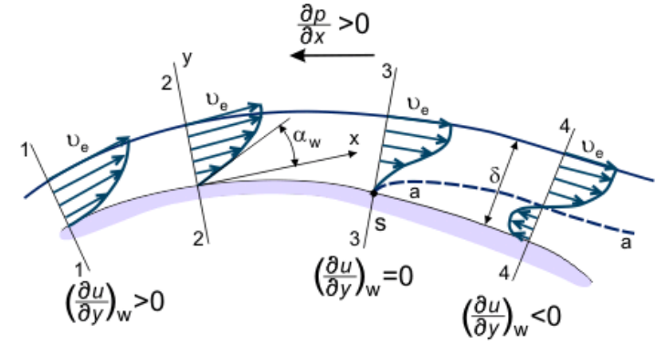
We can see how the velocity gradient in the wall normal direction is initially positive, but then becomes zero at the point of flow separation, turning negative in the recirculation area, where we have no velocity profile pointing against the main flow.

What does this mean for our discussion? Well, let’s look at the definition for the y^+ value:

y^+ = \frac{y u_\tau}{\nu} = \frac{y \sqrt{\frac{\tau_w}{\rho}}}{\nu}\tag{97}

We can see that as \tau_w goes to zero (we approach the point of flow separation), the value for y^+ also goes to zero. This is a problem, as we assumed a logarithmic velocity profile which is only valid for large y^+ values, i.e. typically y^+ > 30. Thus, this approach may start to produce inaccurate results in areas that are crucial to capture correctly, like flow separation.

Therefore, we may be tempted to use a different approach, one which gives us some protection if our y^+ value locally drops into the transition or viscous sublayer. There are a few approaches available, but perhaps two of the most common approaches are given by Spalding and Werner and Wengle. These are schematically shown in the following figure:

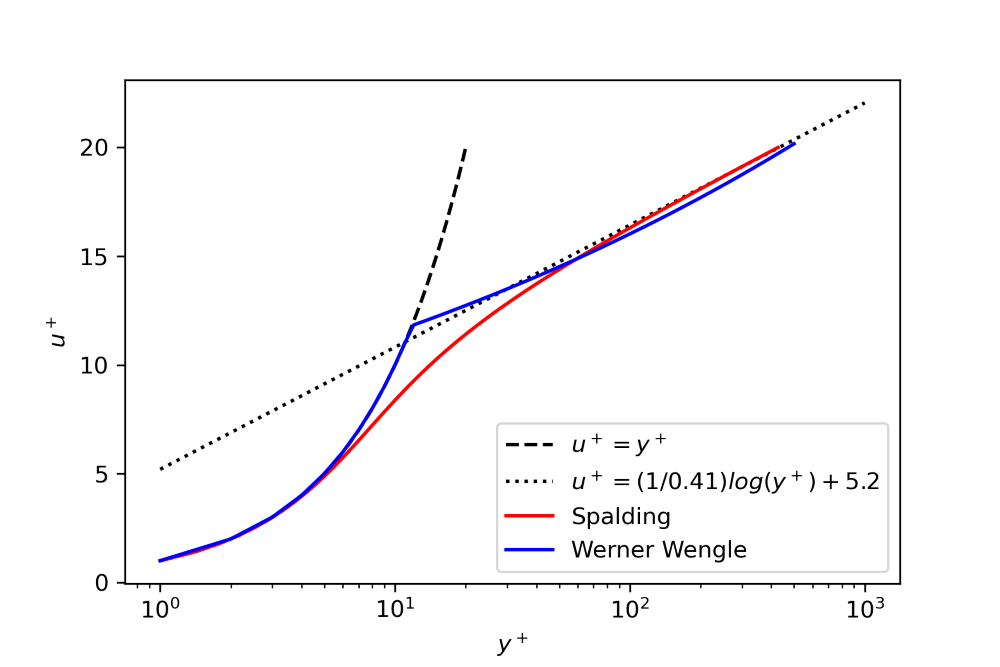
In addition, we also see the two profiles approximating the inner (linear) and outer (logarithmic) layer in this figure. The Spalding function actually provides a really good match with the real velocity profile and is therefore commonly used, not just in WMLES but also in RANS-based wall modelling. We will ignore the Werner and Wengle approximation for the moment; we will return to it in the next section.

Let’s look at Spalding’s wall model first. Given a certain friction velocity u_\tau, the corresponding y^+ value can be obtained, according to Spalding, using the following equation:

y^+ = u^+ + A \left( e^{\kappa u^+} - 1 - \kappa u^+ - \frac{(\kappa u^+)^2}{2} - \frac{(\kappa u^+)^3}{6} \right)\tag{98}

Let’s insert definitions for u^+ and y^+, which results in:

\frac{y u_\tau}{\nu} = \frac{u}{u_\tau} + A \left( e^{\kappa \frac{u}{u_\tau}} - 1 - \kappa \frac{u}{u_\tau} - \frac{(\kappa \frac{u}{u_\tau})^2}{2} - \frac{(\kappa \frac{u}{u_\tau})^3}{6} \right)
\tag{99}

Eq.(99) has the same issue that we had with the logarithmic velocity profile, i.e. we have the friction velocity u_\tau, from which we would obtain wall shear stresses \tau_w, defined on both sides, and we can’t solve for it directly. So, we can use our trusted Newton-Rhapson again, or, if we are lazy, we can just use a root-finding algorithm.

Let’s say we have a function like y = x^3 - x - 2, and we want to know at which point this polynomial will cross the x-axis (or, in other words, at which point y=0). Then, we can move all terms to either the left-hand or right-hand side, e.g. y - x^3 + x + 2 = 0 . This has the effect that one side will contain all the terms from the original equation, and the other side will be equal to zero.

What root finding algorithms will do now is to guess an initial value for x and then update that until we approximately satisfy the equation above, i.e. having a zero right-hand side value (or, y \approx 0 in our original equation). One popular root finding algorithm is the bisect method.

The nice thing about root finding algorithms is that they don’t require us to provide the first derivative of the function, which typically requires us to known the function analytically that we are trying to solve. If that function becomes too complex, we have to resort to either symbolic manipulations using a package like Maple/Matlab (commercial), or SymPy (Python/open-source) or automatic differentiation, which increases complexity (unnecessarily!).

So, let’s see how we can use the bisect method to solve for the friction velocity u_\tau. First, we need to collect all terms on the right-hand side of the equation, and set the left-hand side to zero in Eq.(99). This results in:

0 = \frac{y u_\tau}{\nu} - \frac{u}{u_\tau} - A \left( e^{\kappa \frac{u}{u_\tau}} - 1 - \kappa \frac{u}{u_\tau} - \frac{(\kappa \frac{u}{u_\tau})^2}{2} - \frac{(\kappa \frac{u}{u_\tau})^3}{6} \right)\tag{100}

What the bisect method will do now is to define first an interval within which the solution is expected to be. This means we provide a lower and upper bound for u_\tau. We then take the average of the lower and upper bounds and then check if this new value evaluates our equation to zero. If not, we check the sign of the newly computed solution. If that is the same sign as our lower bound, then we set our new lower bound to the average of the lower and upper bounds. If the sign is opposite, we set the upper bound to the average of the lower and upper bounds.

This ensures that we iteratively reduce the interval until it gets so small that the average of the lower and upper bounds becomes so small that we effectively have converged to a value that does not change anymore. In this case, that would be the friction velocity in our case. This is a high-level overview, and you may want to check the above-linked article on how the bisect method works if you want to understand the method in more detail. The article also comes with a pseudo code for how to implement the bisect method, which I have done below so you don’t have to:

from math import pow, exp, fabs
import numpy as np

def spalding(u, y, nu, u_tau):
  yp = y * u_tau / nu
  up = u / u_tau
  return yp - up - (1/8.6)*(exp(0.41*up) - 1 - 0.41 * up - pow(0.41 * up, 2)/2 - pow(0.41 * up, 3)/6)
  
def bisect_method(u, y, nu, u_tau, max_iterations, tolerance):
  a = u / 1000
  b = 10 * u

  for i in range(1, max_iterations):
    c = (a + b) / 2
    root_of_c = spalding(u, y, nu, c)
    root_of_a = spalding(u, y, nu, a)

    if fabs(b - a)/2 < tolerance:
      u_tau = c
      break

    if (np.sign(root_of_c) == np.sign(root_of_a)):
      a = c
    else:
      b = c

  print(f"Converged u_tau = {u_tau:.6f} after {i} iterations")
  print(f"Computed  y+    = {(y * u_tau / nu):.1f}")
  
# turbulent boundary layer parameters
u = [0.05, 0.2, 1.0]
y = 1e-3
nu = 1e-6

# initial value for u_tau, can be anything
u_tau = 0.01

# bisect iterations
max_iterations = 100
tolerance = 1e-8

# calculate u_tau using the bisect method (root finding)
for u_value in u:
  bisect_method(u_value, y, nu, u_tau, max_iterations, tolerance)

from math import pow, exp, fabs
import numpy as np

def spalding(u, y, nu, u_tau):
  yp = y * u_tau / nu
  up = u / u_tau
  return yp - up - (1/8.6)*(exp(0.41*up) - 1 - 0.41 * up - pow(0.41 * up, 2)/2 - pow(0.41 * up, 3)/6)
  
def bisect_method(u, y, nu, u_tau, max_iterations, tolerance):
  a = u / 1000
  b = 10 * u

  for i in range(1, max_iterations):
    c = (a + b) / 2
    root_of_c = spalding(u, y, nu, c)
    root_of_a = spalding(u, y, nu, a)

    if fabs(b - a)/2 < tolerance:
      u_tau = c
      break

    if (np.sign(root_of_c) == np.sign(root_of_a)):
      a = c
    else:
      b = c

  print(f"Converged u_tau = {u_tau:.6f} after {i} iterations")
  print(f"Computed  y+    = {(y * u_tau / nu):.1f}")
  
# turbulent boundary layer parameters
u = [0.05, 0.2, 1.0]
y = 1e-3
nu = 1e-6

# initial value for u_tau, can be anything
u_tau = 0.01

# bisect iterations
max_iterations = 100
tolerance = 1e-8

# calculate u_tau using the bisect method (root finding)
for u_value in u:
  bisect_method(u_value, y, nu, u_tau, max_iterations, tolerance)

The results from this are:

Converged u_tau = 0.007363 after 26 iterations
Computed  y+    = 7.4
Converged u_tau = 0.018126 after 28 iterations
Computed  y+    = 18.1
Converged u_tau = 0.065910 after 30 iterations
Computed  y+    = 65.9

Converged u_tau = 0.007363 after 26 iterations
Computed  y+    = 7.4
Converged u_tau = 0.018126 after 28 iterations
Computed  y+    = 18.1
Converged u_tau = 0.065910 after 30 iterations
Computed  y+    = 65.9

Spalding’s approach works well and in-fact, gives us a really close match with the real velocity profile. However, for each grid point, we need to obtain the friction velocity through an iterative procedure (Newton-Rhapson, Bisect, other root finding algorithm). While they are not expensive, they certainly add an overhead, and, in the case of the Newton-Rhapson method, would require the derivative of the function to be known in advance.

If we don’t want to iteratively obtain our wall shear stresses, then we need to reformulate the velocity profile in a turbulent boundary layer in a way that we can solve for u_\tau directly. Other people have thought of that already (so you and I have more time to study those important YouTube shorts that the algorithm is recommending us). Let us have a crack at those types of formulations as well in the next section.

Werner Wengle

Werner and Wengle introduced a velocity profile that could be used for both the inner and outer layer of a turbulent boundary layer (i.e. any y^+ value), without the need to find the value for the wall shear stresses iteratively. Clearly, this is lucrative, but as we have already seen, this also comes at a cost. If you refer back to the previous figure where we looked at the different velocity profiles, we see that Werner and Wengle’s profile deviates slightly in the transition region from the smooth transition that we typically have here.

So let us have a look at the velocity profile according to Werner and Wengle. It is given, for the non-dimensional velocity u^+, as:

u^+ = 
\begin{cases}
y^+ & \text{if } y^+ \leq y^+_t \\
A (y^+)^B & \text{if } y^+ \gt y^+_t
\end{cases}
\tag{101}

Here, we have A=8.3 and B=1/7. y^+_t is the y^+ value where we switch from one part of the velocity profile to the other. Werner and Wengle stated it to be:

y^+_t = A^{\frac{1}{1-B}} \approx 11.81
\tag{102}

If you look at other literature, the value for y^+_t may be given as 11, or 11.25. The exact value is not of importance; the take-away message is that it is somewhere around 11, and Werner and Wengle defined it as in Eq.(102). That’s their choice. Feel free to come up with your own value for when you create your own algebraic wall model!

The value of B=1/7 isn’t a coincidence either. If you are dealing with turbulent flows for a while, you will come across the 1/7 power law. A turbulent velocity profile can be computed with this value reasonably well (if you look at the figure above, you’ll notice that the match isn’t perfect, but somewhat good enough).

In the logarithmic velocity plot, we had the friction velocity within the logarithm, i.e. see Eq.(91). This meant that we cannot solve for the friction velocity directly (as it also appears on the left-hand side of the equation), and so an iterative procedure is required.

But, if we replace this logarithmic profile with a power-law, where the friction velocity u_\tau may appear raised to some arbitrary power, we can isolate it again. This means we can derive an explicit equation for u_\tau, and so we no longer need an iterative procedure like the Newton-Raphson or a root finding algorithm. This was the motivation for Werner and Wengle, i.e. throw away the logarithm so that an explicit equation for u_\tau (and thus the wall shear stresses \tau_w) can be found.

Let’s see how they did that. In Eq.(101), we have two cases: the velocity profile in the linear regime, which is just u^+ = y^+, and the velocity profile in the logarithmic layer, which is replaced by the power law u^+ = A(y^+)^B. Let’s look at each part in turn.

To remind ourselves, our goal is to derive an explicit equation for \tau_w, which we get from the friction velocity. So, in the linear regime, we can insert the definitions for u^+ and y^+ into Eq.(101) and get:

u^+ = y^+ \\[1em]
\frac{u}{u_\tau} = \frac{y u_\tau}{\nu}\tag{103}

We multiply by u_\tau:

u = \frac{y u_\tau^2}{\nu}\tag{104}

Now we isolate u_\tau^2 and get:

u_\tau^2 = \frac{u \nu}{y}\tag{105}

We can now insert the definition for the friction velocity, i.e. u_\tau = \sqrt{\tau_w/\rho}. This results in:

\left(\sqrt{\frac{\tau_w}{\rho}}\right)^2 = \frac{u \nu}{y}\tag{106}

The square root and power of two will cancel each other, so we can simply solve for the wall shear stresses now as:

\tau_w = \rho\frac{u \nu}{y}
\tag{107}

If you look at references talking about the Werner Wengle model, then you will often find the following definition instead:

\tau_w = \rho\frac{2u \nu}{\Delta y}\tag{108}

What Werner and Wengle assume here is that we are using a finite volume solver, where the \Delta y is the height of the first cell near the wall, but the centroid is at the centre of this cell, which happens to be at \Delta y/2. However, if you are using a finite difference solver, or you just arrange your control volumes differently, so that your centroids are now coinciding with the cell vertices, then we would have y=\Delta y. Just something to keep in mind.

So far, so good, we got the wall shear stresses with relative ease. As long as we are below the transition y^+_t of y^+_t \approx 11.81, then we can use this relationship …

Did you spot the issue here? Let’s look at the definition of the y^+ value again:

y^+ = \frac{y u_\tau}{\nu} = \frac{y \sqrt{\frac{\tau_w}{\rho}}}{\nu}\tag{109}

The y^+ value itself depends on the wall shear stresses, but we need to compute the y^+ value at the start to know which velocity profile to take (i.e. the linear or power-law profile in Eq.(101)), at a point where we don’t know the wall shear stresses yet. The solution, well, we use a Newton-Rhapson or a root finding algorithm to iteratively find the value of \tau_w and this y^+ …

Great, what’s the point then? Well, we could go the iterative route, but even Werner and Wengle realised that doing so would be too much of a scam (given that the whole point is to replace the iterative procedure). Well, maybe they realised it, or maybe they didn’t; their 1991 paper is very superficial and raises more questions than it provides answers, so it is anyone’s guess what they were thinking about their model.

The route we take is a different one here. Werner and Wengle argued that we can take an average value for u^+ by integrating from the wall to y^+_t and dividing this result by the distance from the wall to y^+_t. If we compute the average velocity, then solving the equation for the wall shear stresses provides us with an averaged wall shear stress value, which is typically what we want to impose as boundary conditions in WMLES. Thus, we get:

u^+ = \frac{1}{y^+_t}\int_0^{y^+_t}y^+\mathrm{d}y^+\tag{110}

We integrate over y^+ as we have the relationship u^+ = y^+ for the linear regime (viscous sublayer). Carrying out the integration results in:

u^+ = \frac{1}{y^+_t}\left[\frac{y^{+^2}}{2}\right]\biggr\rvert_0^{y^+_t}\tag{111}

Inserting the integration bounds, we get:

u^+ = \frac{1}{y^+_t}\left[\frac{y^{+^2}_t}{2} - \frac{0}{2}\right] = \frac{1}{2y^+_t}y^{+^2}_t\tag{112}

We can now insert the definition for y^+_t = A^{1/(1-B)}, where two numbers raised to a power combine through multiplication. Thus, we get:

u^+ = \frac{1}{2y^+_t}\left(A^{\frac{1}{1-B}}\right)^2 = \frac{1}{2y^+_t}A^{\frac{2}{1-B}}
\tag{113}

Let’s insert the definition for u^+ and y^+:

\frac{u}{u_\tau} = \frac{\nu}{2 y u_\tau}A^{\frac{2}{1-B}}\tag{114}

Now let’s multiply both sides by the friction velocity u_\tau, and we get:

u = \frac{\nu}{2 y}A^{\frac{2}{1-B}}
\tag{115}

Now what does Eq.(115) tell us? Well, it tells us what velocity u we should be expecting to prevail at y^+_t. Thus, if we evaluate the wall shear stresses from properties found at a certain height h from the wall, we first check the velocity u. If it is smaller than the velocity computed from Eq.(115), we know we are below y^+_t. if it is larger, then we must be above y^+_t. This completely removes the need to compute the y^+ value, and so further dependence on u_\tau is removed.

Ok, but what happens in the logarithmic layer? Let’s have a look. First, we compute the average velocity again so that we can relate the average velocity to the average wall shear stresses. To do that, we first have to integrate the linear (viscous sublayer) all the way from the wall to the transition y^+_t value, and then from this value all the way to the height y^+_h at which we seek to evaluate the velocity profile. This results in the following integral:

u^+=\underbrace{\frac{1}{y^+}\int_{0}^{y^+_t}y^+\mathrm{d}y^+}_{\text{viscous sublayer}} + \underbrace{\frac{1}{y^+}\int_{y^+_t}^{y^+_h}A(y^+)^B\mathrm{d}y^+}_{\text{logarithmic sublayer}}\tag{116}

We already know what the viscous sublayer evaluates to, e.g. see Eq.(113), let us write out the integral with this term inserted:

u^+=\underbrace{\frac{1}{2y^+}A^{\frac{2}{1-B}}}_{\text{viscous sublayer}} + \underbrace{\frac{1}{y^+}\int_{y^+_t}^{y^+_h}A(y^+)^B\mathrm{d}y^+}_{\text{logarithmic sublayer}}
\tag{117}

Now let’s focus on the second term. This can be integrated as:

\frac{1}{y^+}\int_{y^+_t}^{y^+_h}A(y^+)^B\mathrm{d}y^+ = \left[\frac{1}{y^+}\frac{A}{1+B}(y^+)^{B+1}\right]\biggr\rvert_{y^+_t}^{y^+_h} = 
\left[\frac{1}{y^+}\frac{A}{1+B}\left((y^+_h)^{B+1} - (y^+_t)^{B+1}\right)\right]\tag{118}

For the second term, let us replace y^+_t=A^{1/(1-B)}. This results in:

\left[\frac{1}{y^+}\frac{A}{1+B}\left((y^+_h)^{B+1} - (y^+_t)^{B+1}\right)\right] = \left[\frac{1}{y^+}\frac{A}{1+B}\left((y^+_h)^{B+1} - A^{\frac{B+1}{1-B}}\right)\right]\tag{119}

For the first term, let us introduce the definition for the y^+ value, which results in:

\left[\frac{1}{y^+}\frac{A}{1+B}\left((y^+_h)^{B+1} - A^{\frac{B+1}{1-B}}\right)\right] = \left[\frac{1}{y^+}\frac{A}{1+B}\left((\frac{y u_\tau}{\nu})^{B+1} - A^{\frac{B+1}{1-B}}\right)\right] = \frac{1}{y^+}\frac{A}{1+B} \left(\frac{y u_\tau}{\nu}\right)^{B+1} - \frac{1}{y^+}\frac{A}{1+B} A^{\frac{B+1}{1-B}}\tag{120}

Let is insert this final form into Eq.(117), this results in:

u^+=\frac{1}{2y^+}A^{\frac{2}{1-B}} + 
\frac{1}{y^+}\frac{A}{1+B} \left(\frac{y u_\tau}{\nu}\right)^{B+1} - \frac{1}{y^+}\frac{A}{1+B} A^{\frac{B+1}{1-B}}\tag{121}

Now we multiply by y^+, which gives us the following equation:

u^+ y^+=\frac{1}{2}A^{\frac{2}{1-B}} + \frac{A}{1+B} \left(\frac{y u_\tau}{\nu}\right)^{B+1} - \frac{A}{1+B} A^{\frac{B+1}{1-B}}\tag{122}

Now we insert the definitions for u^+ and y^+ and obtain:

\frac{u}{u_\tau} \frac{y u_\tau}{\nu}=\frac{1}{2}A^{\frac{2}{1-B}} + \frac{A}{1+B} \left(\frac{y u_\tau}{\nu}\right)^{B+1} - \frac{A}{1+B} A^{\frac{B+1}{1-B}} = \\[1em]
u \frac{y}{\nu}=\frac{1}{2}A^{\frac{2}{1-B}} + \frac{A}{1+B} \left(\frac{y u_\tau}{\nu}\right)^{B+1} - \frac{A}{1+B} A^{\frac{B+1}{1-B}}
\tag{123}

We can see that u_\tau cancels on the left-hand side, but we still have u_\tau on the right-hand side. We can isolate u_\tau using the following identity:

(\phi\psi)^\alpha \rightarrow \phi^\alpha \psi^\alpha \\[1em]
\left(\frac{y u_\tau}{\nu}\right)^{1+B} = u_\tau^{1+B} \left(\frac{y}{\nu}\right)^{1+B}\tag{124}

If we insert that into Eq.(123), then we obtain:

u \frac{y}{\nu}=\frac{1}{2}A^{\frac{2}{1-B}} + \frac{A}{1+B} u_\tau^{1+B} \left(\frac{y}{\nu}\right)^{1+B} - \frac{A}{1+B} A^{\frac{B+1}{1-B}}\tag{125}

We can solve this expression now directly for u_\tau. First, we multiply by (1+B)/A, which results in:

\frac{1+B}{A} u \frac{y}{\nu}= \frac{1+B}{A} \frac{1}{2}A^{\frac{2}{1-B}} + u_\tau^{1+B} \left(\frac{y}{\nu}\right)^{1+B} - \frac{1+B}{A}\frac{A}{1+B} A^{\frac{B+1}{1-B}} \\[1em]
\frac{1+B}{A} u \frac{y}{\nu}= \frac{1+B}{A} \frac{1}{2}A^{\frac{2}{1-B}} + u_\tau^{1+B} \left(\frac{y}{\nu}\right)^{1+B} - A^{\frac{B+1}{1-B}}
\tag{126}

Next, we need to multiply by the inverse of (y/\nu)^{1+B} to isolate u_\tau. This is achieved by multiplying by the reversed fraction, i.e.:

\frac{1}{\left(\frac{\phi}{\psi}\right)^\alpha} = \left(\frac{\psi}{\phi}\right)^\alpha \tag{127}

Therefore, we multiply Eq.(126) by (\nu/y)^{1+B} and get:

\frac{1+B}{A} u \frac{y}{\nu}\left(\frac{\nu}{y}\right)^{1+B}= \frac{1+B}{A} \frac{1}{2}A^{\frac{2}{1-B}}\left(\frac{\nu}{y}\right)^{1+B} + u_\tau^{1+B} - A^{\frac{B+1}{1-B}}\left(\frac{\nu}{y}\right)^{1+B}
\tag{128}

Let’s look at the first term on the left-hand side. Using the exponent rule \phi^\alpha\phi^\beta = \phi^{\alpha + \beta}, we can simplify this term as:

\frac{1+B}{A} u \frac{y}{\nu}\left(\frac{\nu}{y}\right)^{1+B} =
\frac{1+B}{A} u \frac{y}{\nu}\left(\frac{\nu}{y}\right)^{1}\left(\frac{\nu}{y}\right)^{B} = 
\frac{1+B}{A} u \left(\frac{\nu}{y}\right)^{B}\tag{129}

Let’s insert this into Eq.(128) and isolate u_\tau^{1+B}. This results in:

u_\tau^{1+B} = \frac{1+B}{A} u \left(\frac{\nu}{y}\right)^{B} - \frac{1+B}{A} \frac{1}{2}A^{\frac{2}{1-B}}\left(\frac{\nu}{y}\right)^{1+B} + A^{\frac{B+1}{1-B}}\left(\frac{\nu}{y}\right)^{1+B}\tag{130}

We can now raise each term to the power of 1/(1+B); this removes the exponent on the left-hand side. This results in:

u_\tau = \left[\frac{1+B}{A} u \left(\frac{\nu}{y}\right)^{B} - \frac{1+B}{A} \frac{1}{2}A^{\frac{2}{1-B}}\left(\frac{\nu}{y}\right)^{1+B} + A^{\frac{B+1}{1-B}}\left(\frac{\nu}{y}\right)^{1+B}\right]^{\frac{1}{1+B}}\tag{131}

We are now in a position to compute the wall shear stresses directly. For that, we insert the definition of the friction velocity, i.e. u_\tau=\sqrt{\tau_w/\rho}. To make things easier, let’s first solve this expression for \tau_w; this results in \tau_w = \rho u_\tau^2. Now we insert the definition for u_\tau here, as obtained above, and we get the final expression for our wall shear stresses as:

\tau_w = \rho\left[\frac{1+B}{A} u \left(\frac{\nu}{y}\right)^{B} - \frac{1+B}{A} \frac{1}{2}A^{\frac{2}{1-B}}\left(\frac{\nu}{y}\right)^{1+B} + A^{\frac{B+1}{1-B}}\left(\frac{\nu}{y}\right)^{1+B}\right]^{\frac{2}{1+B}}
\tag{132}

Notice how the exponent for the term on the right-hand side changed from 1/(1+B) to 2/(1+B) as we have to square the friction velocity u_\tau. If you look at the literature, you may find a slightly shorter form of this expression, where the second and third terms are combined, but in the end, they compute the same thing.

We said that the equation for the velocity profile in the viscous sublayer (and beginning of the transition region) is evaluated by Eq.(107), i.e. for y^+ \lt 11.81. Since we wanted to stay explicit in the evaluation of the wall shear stresses, we computed the maximum velocity instead of the wall shear stresses in Eq.(115) to determine if we are above or below this transitional y^+ value.

Using the definition of the velocity at which we are above/below y^+_t=11.81 (Eq.(115)), as well as the wall shear stresses for the viscous sublayer (Eq.(107)) and the logarithmic layer (Eq.(132)), we can now rewrite the original definition by Werner and Wengle for the velocity profile as given in Eq.(101). Instead of writing this now for the non-dimensional velocity u^+, we express it in terms of the wall shear stresses \tau_w as:

\tau_w = 
\begin{cases}
\rho\frac{u \nu}{y} & u \leq \frac{\nu}{2 y}A^{\frac{2}{1-B}} \\[1em]
\rho\left[\frac{1+B}{A} u \left(\frac{\nu}{y}\right)^{B} - \frac{1+B}{A} \frac{1}{2}A^{\frac{2}{1-B}}\left(\frac{\nu}{y}\right)^{1+B} + A^{\frac{B+1}{1-B}}\left(\frac{\nu}{y}\right)^{1+B}\right]^{\frac{2}{1+B}} & u \gt \frac{\nu}{2 y}A^{\frac{2}{1-B}}
\end{cases}
\tag{133}

In this expression, I have left the variable y here, instead of inserting \Delta y/2 for it, which would only be applicable to cell centered discretisations. If that is what you are doing, set y=\Delta y/2. If you are evaluating your unknowns at the vertices, then set y=\Delta y. If you are using a staggered grid arrangement, with information stored both at cell centers and face centres, then don’t use a staggered approach (it is not defined in this case, but also, staggered discretisations belong in the classroom, not in your CFD solver).

Of course, we can implement that again into a simple Python code and check what values we get with this model (setting y=\Delta y here). The code below shows how the wall shear stresses are explicitly computed using Eq.(133):

from math import pow, sqrt

def werner_wengle_viscous_sublayer(rho, u, nu, y):
  return rho * (u * nu / y)

def werner_wengle_log_layer(rho, u, nu, y, A, B):
  term_1 = ((1+B)/A) * u * pow(nu / y, B)
  term_2 = ((1+B)/A) * 0.5 * pow(A, 2/(1-B)) * pow(nu / y, B+1)
  term_3 = pow(A, (B+1)/(1-B)) * pow(nu / y, B+1)
  return rho * pow(term_1 - term_2 + term_3, 2/(1+B))

# werner wengle
# turbulent boundary layer parameters
u = [0.05, 0.2, 1.0]
y = 1e-3
nu = 1e-6
rho = 1

A = 8.3
B = 1.0/7.0

# calculate wall shear stresses analytically
for u_value in u:
  u_critical = (nu / (2 * y))*pow(A, 2/(1-B))
  if u_value <= u_critical:
    tau_w = werner_wengle_viscous_sublayer(rho, u_value, nu, y)
  elif u_value > u_critical:
    tau_w = werner_wengle_log_layer(rho, u_value, nu, y, A, B)

  u_tau = sqrt(tau_w/rho)

  print(f"Computed u_tau = {u_tau:.6f}")
  print(f"Computed y+    = {(y * u_tau / nu):.1f}")

from math import pow, sqrt

def werner_wengle_viscous_sublayer(rho, u, nu, y):
  return rho * (u * nu / y)

def werner_wengle_log_layer(rho, u, nu, y, A, B):
  term_1 = ((1+B)/A) * u * pow(nu / y, B)
  term_2 = ((1+B)/A) * 0.5 * pow(A, 2/(1-B)) * pow(nu / y, B+1)
  term_3 = pow(A, (B+1)/(1-B)) * pow(nu / y, B+1)
  return rho * pow(term_1 - term_2 + term_3, 2/(1+B))

# werner wengle
# turbulent boundary layer parameters
u = [0.05, 0.2, 1.0]
y = 1e-3
nu = 1e-6
rho = 1

A = 8.3
B = 1.0/7.0

# calculate wall shear stresses analytically
for u_value in u:
  u_critical = (nu / (2 * y))*pow(A, 2/(1-B))
  if u_value <= u_critical:
    tau_w = werner_wengle_viscous_sublayer(rho, u_value, nu, y)
  elif u_value > u_critical:
    tau_w = werner_wengle_log_layer(rho, u_value, nu, y, A, B)

  u_tau = sqrt(tau_w/rho)

  print(f"Computed u_tau = {u_tau:.6f}")
  print(f"Computed y+    = {(y * u_tau / nu):.1f}")

Running this code will produce the following results:

Computed u_tau = 0.007071
Computed y+    = 7.1
Computed u_tau = 0.022296
Computed y+    = 22.3
Computed u_tau = 0.077790
Computed y+    = 77.8

Computed u_tau = 0.007071
Computed y+    = 7.1
Computed u_tau = 0.022296
Computed y+    = 22.3
Computed u_tau = 0.077790
Computed y+    = 77.8

At this point, we can compare all three methods (standard logarithmic wall function, Spalding, and Werner and Wengle), and see how they compare, both in terms of computational cost (number of iterations required to iteratively compute the wall shear stresses, if applicable) and values obtained. A comparison of all of these results is done below:

For u=0.05, we get:

# Logarithmic velocity profile
Converged u_tau = 0.005375 after 7 iterations
Computed  y+    = 5.4

# Spalding
Converged u_tau = 0.007363 after 26 iterations
Computed  y+    = 7.4

# Werner and Wengle
Computed u_tau = 0.007071
Computed y+    = 7.1

# Logarithmic velocity profile
Converged u_tau = 0.005375 after 7 iterations
Computed  y+    = 5.4

# Spalding
Converged u_tau = 0.007363 after 26 iterations
Computed  y+    = 7.4

# Werner and Wengle
Computed u_tau = 0.007071
Computed y+    = 7.1

For u=0.2, we get:

# Logarithmic velocity profile
Converged u_tau = 0.016595 after 5 iterations
Computed  y+    = 16.6

# Spalding
Converged u_tau = 0.018126 after 28 iterations
Computed  y+    = 18.1

# Werner and Wengle
Computed u_tau = 0.022296
Computed y+    = 22.3

# Logarithmic velocity profile
Converged u_tau = 0.016595 after 5 iterations
Computed  y+    = 16.6

# Spalding
Converged u_tau = 0.018126 after 28 iterations
Computed  y+    = 18.1

# Werner and Wengle
Computed u_tau = 0.022296
Computed y+    = 22.3

For u=1.0, we get:

# Logarithmic velocity profile
Converged u_tau = 0.065012 after 8 iterations
Computed  y+    = 65.0

# Spalding
Converged u_tau = 0.065910 after 30 iterations
Computed  y+    = 65.9

# Werner and Wengle
Computed u_tau = 0.077790
Computed y+    = 77.8

# Logarithmic velocity profile
Converged u_tau = 0.065012 after 8 iterations
Computed  y+    = 65.0

# Spalding
Converged u_tau = 0.065910 after 30 iterations
Computed  y+    = 65.9

# Werner and Wengle
Computed u_tau = 0.077790
Computed y+    = 77.8

As we can see, within the viscous sublayer (y^+ \approx 5), the logarithmic profile underpredicts the friction velocity significantly, which would result in reduced wall shear stresses. If we are interested in capturing flow separations accurately here, then the pure logarithmic velocity profile will likely be insufficient. Both Spalding and Werner and Wengle agree well here.

Within the transition region (y^+ \approx 20), all profiles provide reasonable agreement. The logarithmic profile may not yet be fully valid, but it is in line with what Spalding and Werner and Wengle predict; it certainly performs much better than in the viscous sublayer, as expected.

In the log layer (y^+ \approx 65), we have pretty good agreement between the logarithmic velocity formulation and Spalding’s approach. Werner and Wengle are a bit off here, though we still get a fairly good match (let’s not forget that this fairly good agreement comes with the advantage that we do not have to iteratively find the value for the wall shear stresses).

While there are quite a few more ways to obtain the wall shear stresses in WMLES, I’ll stop here. The main reason is that the additional approaches that exist in the literature seem to be fairly academic, i.e. they are well defined, derived, and they work, but they offer no real advantage over the approaches described above.

For that reason, you’ll likely find most people dealing with one of the three approaches we have looked at here, unless you are doing research on WMLES and you try to improve the methodology itself. But, for the rest of us, who want to use WMLES to solve real problems, sticking with the above approaches will be sufficient for all of our simulation needs.

Meshing requirements for hybrid RANS/LES approaches

We have gone through quite a bit of theory, but none of that will matter if our grid is not aligned with what our turbulence model needs. The grid requirements are similar for all turbulence modelling approaches, but differ in small but important ways. Thus, in this section, we will look at what grid requirements to ensure our turbulence modelling approach will provide us with accurate simulations.

I should stress here that these are experiential values, gathered from various academic publications as well as personal experiences. See these as a starting point. Using these meshing guidelines will not free you from performing validation studies, e.g. comparing your simulations against experiments or other high-fidelity CFD simulations.

Detached Eddy Simulations (DES)

When Spalart introduced his DES approach, he stated that the near-wall treatment is driven entirely by the turbulence model itself. He used the Spalart-Allmaras turbulence model, which requires a near-wall spacing of \Delta y^+=1. If we were to use the k-\omega SST model, for example, which can be used for both \Delta y^+=1 and \Delta y^+ \gt 30 for the first cell height, then this would determine our mesh in the wall normal direction.

In practice, though, the standard DES formulation suffers from grid-induced separation (GIS), as discussed in the DES section, and so a \Delta y^+ value of 1 is typically adopted here. In terms of streamwise and spanwise grid-spacing, i.e. \Delta x^+ and \Delta z^+, we have two cases to consider.

For the RANS portion of the flow, there is no limit, i.e. we can stretch our cells as much as we want. For the LES portion of the flow, however, i.e. anything outside the boundary layer, we want to limit the cell sizes in the spanwise and streamwise direction. A good initial starting point tends to be around 100 \le \Delta x^+ \le 200 (streamwise, i.e. in flow direction) while we have 30 \le \Delta z^+ \le 100 in the spanwise direction (perpendicular to the flow and parallel to the wall).

Having said that, it is typically prudent to perform a grid convergence study on a pure, steady-state, RANS simulation to determine the spacing in each direction, and then using this grid for the DES simulations. We would also typically start the DES simulation from the steady-state RANS simulation as the initial solution.

Delayed Detached Eddy Simulations (DDES) / Improved Delayed Detached Eddy Simulations (IDDES)

The grid requirements for DDES and IDDES are the same as DES, i.e. it follows RANS meshing guidelines. However, both DDES and IDDES remove the issue of grid-induced separation (DES), while IDDES also remove the logarithmic layer mismatch in the outer layer of the boundary layer. Thus, the turbulence modelling approach is much more robust compared to DES, which allows us to relax our meshing requirements.

While it may still make sense to use a \Delta y^+ value of 1, for example, to capture free separation over curved surfaces (e.g. airfoils), we can substantially reduce this if we wanted and only capture the outer (logarithmic) layer of the boundary layer. This translates to a first cell height requirement of 30 \le \Delta y^+ \le 100. If we opt for this treatment, we would still try, though, to place approximately 10-15 cells within the boundary layer.

In terms of spanwise and streamwise direction, the same limits as discussed in the previous section on DES applies here.

Scale-adaptive Simulations (SAS)

SAS is really just a URANS approach, which typically is extended into the hybrid RANS/LES regime. Therefore, we typically require \Delta y^+ to be of the order of 1, while we have similar meshing requirements ion the spanwise and streamwise direction compared to DES/DDES/IDDES. Since \Delta y^+ can be much smaller than in DDES and IDDES in particular, we may want to reduce the streamwise spacing 50 \le \Delta x^+ \le 150.

We may want to reduce the spacing in the spanwise direction as well, though to keep the mesh size somewhat manageable, we may justify leaving the grid requirements here to something similar as in DES/DDES/IDDES. This will largely depend on your flow. If you are expecting cross flow within the boundary layer (e.g. studying wing tip vortices), then you may want to, at least locally, reduce the spanwise spacing in regions of interest.

Wall-modelled Large Eddy Simulations (WMLES)

For WMLES, as the name suggest, we model the flow near the wall, resulting in reduced grid requirements here. This means that for the first cell height, we typically set 30 \le \Delta y^+ \le 300. This provides rather large savings in the wall-normal direction and makes WMLES a lucrative alternative to standard LES (and even DES/DDES/IDDES/SAS).

In terms of the streamwise and spanwise direction, these are largely driven by LES-grid requirements, and so we may adopt similar grid requirements here. As a starting point, use the same meshing guidelines as DES, but you can coarsen the spacing in the streamwise direction if there is a slow streamwise evolution of the flow.

Summary

We have reached the end of not just this article, but also our mini-series on how to deal with turbulence modelling in CFD codes. We looked at the origin of turbulence and how to capture it exactly using Direct Numerical Simulations (DNS), and then we looked at the various modelling approaches and their complexities, starting with Large Eddy simulations (LES), then looking at Reynolds-averaged Navier-Stokes (RANS) modelling, and finally, in this article, how to combine LES and RANS into so-called hybrid RANS/LES approaches.

In addition, we have also looked at how to capture transition in this article using RANS models. For complex engineering applications, we may want to get a better idea of when the flow separates. However, in practice, transition-based RANS models have very strict mesh requirements (y^+\ll 1, with a slow growth rate of subsequent layers, typically increasing in size of about 1.05). This makes them far less used than you would probably expect, given their presumably superior treatment of turbulence.

With modelling complexity comes uncertainties, and transitional-based RANS models will give you a result, but validation and verification become even more important than for RANS models. Boundary conditions will also become increasingly more important. For example, with standard RANS, you can get away with a simple Dirichlet/Neumann type combination at solid walls, but for transitional-based RANS modelling, you probably also want to account for surface roughness (which will have a significant influence on your results).

This is true in general, i.e. as we go from RANS to transitional RANS, to hybrid RANS/LES, to LES, to DNS, we will have to be more and more careful how we impose boundary conditions. We already looked at surface roughness, but with scaled-resolved simulations (hybrid RANS/LES, LES, DNS), we also need to think about how we impose a realistic inflow condition that has the required turbulence intensity, with a realistic (divergence-free) distribution of turbulent eddies.

The further we increase the mesh, the more turbulence we can resolve using a scale-resolving approach, the more we have to account for additional uncertainties, increased computational cost, willingness to debug our simulation set up if it just doesn’t give us the results we want, resilience in testing boundary conditions; you’ll likely have to trade your soul or sanity to get somewhat reasonable results.

But it is not all that bad! I make turbulence modelling look grim, dark, and like a field where researchers descend into the abyss. But it can be an incredibly rewarding field to work in as well. For the foreseeable future, we will always be limited by computational resources, and so unless we can routinely perform DNS at high-Reynolds number on our smart-fridge, there will always be research grants, projects, and engineering jobs that require people with in-depth knowledge of turbulence modelling.

If you are just getting into turbulence right now, then prepare to be hit left, right, and centre with literature that just doesn’t make sense. I get it, I was there, I know the pain and journey. But once you emerge on the other side and are no longer scared of an integral, you enjoy looking at turbulent boundary layers along flat plates (yawn), and perhaps even interacting with the enemy (aka the common wind tunnel goblin), then working in the area of turbulence is immensely satisfying.

I have written these introductory articles on turbulence to get you set up and started. With the knowledge you have gained in these articles, you should be able to take them to the next level and really immerse yourself in a specific niche.

One last point, before I let you go: If you actually ever introduce the HYDDIES hybrid RANS/LES model, or you even just implement the STUPID RANS model because you hate yourself (?) or have too much time (?), I would be very interested. Get in touch, my Snapchat handle is @Kolmogorov.

---

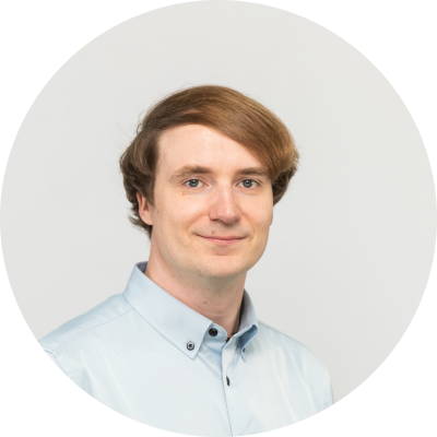
Tom-Robin Teschner is a senior lecturer in computational fluid dynamics and course director for the MSc in computational fluid dynamics and the MSc in aerospace computational engineering at Cranfield University.