Eigen: The Swiss Army Knife of CFD libraries
A new series, a new excuse for me to spend even more hours diving deep into coding and talking about a guilty pleasure of mine. In this new series, I want to highlight and demonstrate C++ libraries that have my life a lot easier when writing CFD solvers in the past, and that will help you write better CFD solvers as well.
The examples I'll provide are taken from real-life use cases where I have used these libraries myself, and the first library we look at is the one library I cannot live without anymore: I am talking about Eigen.
Eigen is, at its core, just a linear algebra library. But, as we will explore together in this article, it can be used for essentially anything that vaguely operates on vectors and matrices. We'll start by looking at basic examples for how to work with vectors and matrices, but then very quickly dive into examples that show how I would use Eigen in a real CFD solver.
We look at examples like discretising PDEs and computing the laplacian within a Poisson solver, computing gradients on unstructured grids using the least-square method (and related methods), computing and storing geometric cell/face information for unstructured solvers, solving linear system fo equations, i.e. [katex]\mathbf{Ax}=\mathbf{b}[/katex], easily computing the CFL number, and, how to compute derivatives exactly, down to machine precision.
Eigen can do all of that, and more, and in this article, I hope to convince you to learn Eigen and use it for your own projects as well. The best part: Eigen is so simple to use that you don't really have to learn it. You just use it. It has an extremely easy API interface, and even if you do get stuck, it probably has one of the best library documentations I have seen in a long time.
So, are you ready to become a better, more proficient CFD programmer? Then this article is for you!
Download Resources
All developed code and resources in this article are available for download. If you are encountering issues running any of the scripts, please refer to the instructions for running scripts downloaded from this website.
- Download: Eigen examples
In this series
[custom_category_posts_list category_slug="essential-libraries-for-cfd-solver-development"]In this article
- Introduction
- Installing Eigen and the example code
- Code examples for Eigen
- Basic Eigen usage examples
- CFD-specific examples
- Computing the CFL number
- Computing geometric information: The Triangle-Point example
- Discretising partial differential equations with Eigen
- Interfacing Eigen with other data types
- Computing gradients on unstructured grids using the least-squares and related approaches
- Working with sparse matrices (and where to best enjoy royal milk tea)
- Using Eigen to solve linear systems of equations
- Computing the flux Jacobian using automatic differentiation
- Summary
Introduction
Whenever we start writing a significant piece of code (and I consider CFD solvers to fall in this category), we rarely want to reinvent the wheel ourselves, meaning, unless we have to, we want to make use of other people's code in the form of libraries, to reduce the amount of code we have to write. This allows us to concentrate on the core logic of our code and then delegate, where we can. There are many reasons why this is beneficial, but these are probably the most important ones:
- Library code, especially high-quality libraries that have rigorous software testing in place, providing you with some degree of confidence that the library is doing what you expect it to. Calling a function from a third-party library is easier than implementing, testing, and maintaining that function yourself.
- Even if bugs exist in that library, you can either report a bug yourself or, for a large enough user community, others will likely come across that bug and request a bug fix themselves. If you regularly update your dependencies (all the libraries you are using), chances are you'll never have to worry about external bugs.
- Libraries are often written by domain experts. You tap into their knowledge, and even if you don't use all the library has to offer, the parts that you do end up using are likely a better implementation to whatever you could ever come up with.
- Library code is often optimised, and an implementation you can come up with may not be as fast and efficient as the library code.
- If you plan to collaborate with other people on your code, using common libraries will help others to find their way around in your codebase. Even if they don't know the library, they can pick it up quickly by referring to the library's documentation, which, let's be honest, will be better than whatever development guide you put together.
- The best part is: You get all of this for free. Forever. You can download the libraries without having to pay for them, and you enjoy all of the benefits stated above. Where else do you get that? Imagine the pharmaceutical industry uploading their recipes for creating drugs to cure cancer, for free, to the internet. We don't often acknowledge this fact, but free and open-source (FOSS) software is a remarkable concept!
Despite these, in my view, overwhelmingly positive advantages, many people, especially when they are starting out with code development, opt for doing everything by themselves, setting them up for failure. I'm not judging; this pretty much describes my personal learning path (and that of those around me when I learned programming and CFD).
I have come to realise that learning a new library is easy, but getting a library integrated into your project is probably the hardest part. And worst of all, some of the most well-known, most-used libraries in CFD simply stick up their middle finger, essentially telling you: "if you can't integrate me into your project, you don't deserve to make use of my capabilities".We'll get around to this particular problem child eventually in this series.
If your first steps with third-party libraries are with one of those libraries that are not very developer-friendly, chances are you give up and just try to write all the code yourself. But then there are these libraries that really stick out from the sea of libraries. They are like a good friend, holding your hand and telling you, "everything will be OK". These are the friends you keep around, and the same is true for libraries, some of them, well, I can't live without.
My last series 10 key concepts everyone must understand in CFD started as a list of topics I wanted to discuss and though are essential to master CFD. My list contained, originally, 9 items, and I thought, "I'll just come up with the last remaining topics as I write this series". Poor planning on my behalf ...
I eventually did come up with the last remaining topic (which was high-performance computing). I had a few topics to pick from, including the role of software engineering in CFD, though that, perhaps, could be explored in a separate series and in a lot more practical terms.
Be that as it may, I have learned from my mistakes, and so for this, brand spanking new series, I have done some soul-searching and thought about which libraries I want to cover in this series. Looking at that list, there is one library in particular I just can't live without; it is my BFF in the world of liraries.
I am talking about Eigen, which is also referred to as Eigen3, even though it is now on version 5 (curiously, there is no version 4. What happened here?).
Eigen is a high-performance, header-only C++ template library for linear algebra applications, providing matrix and vector types, as well as operations you can perform on matrices and vectors. This includes decompositions, computing eigenvalues and eigenvectors (duh, its sort of in the name), as well as solving linear system of equations. On top of that, it does come with some additional features you wouldn't necessarily expect in a linear algebra library, and we will get around to those features as well in this article.
The best part about Eigen is that you don't really have to learn it. Sure, the documentation is there if you need it (although, it seems whenever I want to look something up, gitlab (where the documentation is hosted), is faking an aneurysm and the documentation can't be found), but the library interface is so well designed that with intellisense set up in your code editor, you can start writing code without having to consult the documentation. It is that good!
And this also describes how I got to learn Eigen. I was once working on a solver where Eigen was used. I didn't know the library back then, but I had to start using it. Just by looking at the code that was using Eigen, I immediately understood what the library was doing, and I started using it.
When I started working on my own projects, I just continued to use Eigen. It was such a natural thing to use, and so, when I say, Eigen is the library I can't live without, I mean it (no clickbait). I use it all the time.
The fact that it is header-only also means that you can simply download the library and place it in your project, no additional steps required. You can simply start using it, and your compiler will then compile those parts of Eigen that you are using; no compilation of the library is required ahead of time.
Since it is header-only, it also means that liberal use of templates is allowed, and let me tell you, Eigen is template-galore! Templates are brilliant once you understand them (they have a step learning curve), and they offer optimisation potential at compile-time that is quite impressive.
As the end-user, though, we don't really have to worry about templates, but we will touch upon template vs. non-template code later, as Eigen does provide support for both, and each approach has its own advantages and disadvantages. But I leave that for later when we actually look at code.
So, hopefully, I have successfully whet your appetite for Eigen. It is one of those libraries you will come to love and use in all of your projects. So in the remainder of this article, I want to show you some examples that demonstrate how to use Eigen in the context of CFD solver development.
We'll be using it to compute gradients on unstructured grids, compute geometric information for triangular mesh elements in 3D space, solve a fully implicit partial differential equation, and compute the flux Jacobian exactly without round-off or discretisation errors. And these are just some of the things you can do with Eigen, but hopefully this will help you get an idea of what is possible.
Before we jump into our code examples, let us look at how we can install the library first.
Installing Eigen and the example code
There are two ways of how you can test Eigen, as well as the code samples provided in this article. The first is the easiest, where you can do everything in your browser. The second option requires you to install all dependencies onto your PC, though with the right tools, this can be automated, and it is pretty painless.
You can download all code examples that are used in this article from the link provided at the beginning of the article.
Using Eigen online
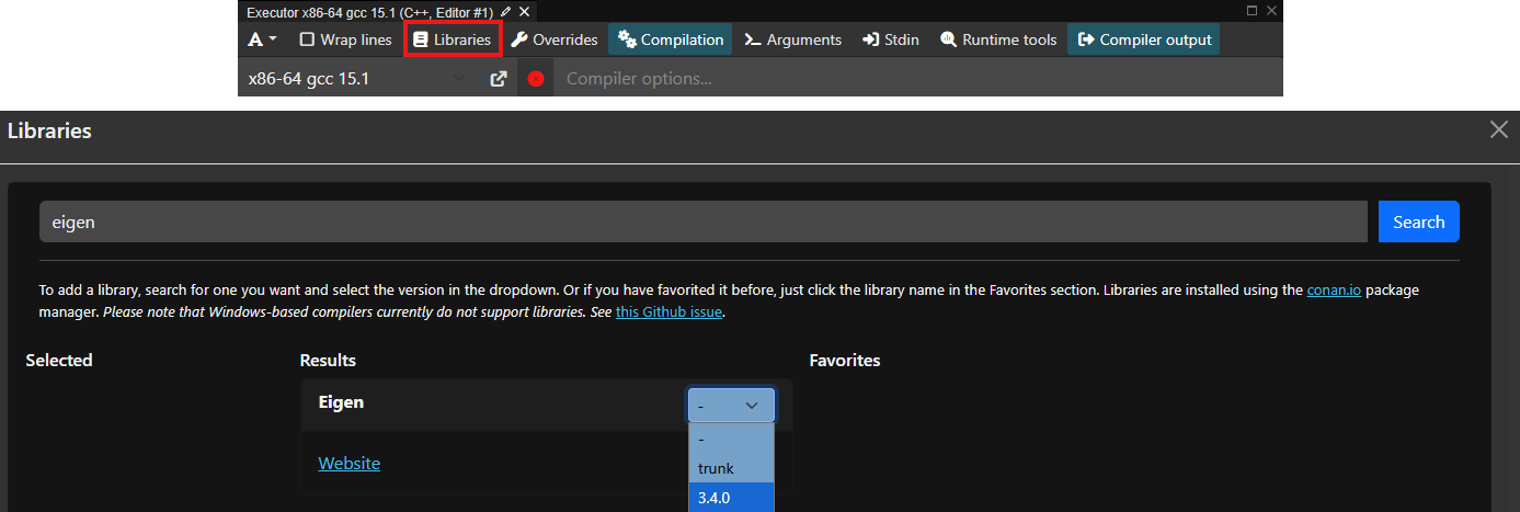
If you just want to play around with Eigen, the easiest way is to head over to compiler explorer, activating Eigen as a project dependency, and start coding. To activate Eigen, click on the Libraries button as shown below (red rectangle), and type eigen in the window that appears (shown below). Select the version you want to use; 3.4.0 is the latest as of the time of writing, which has been stable for some time and all examples will work with this version.
To test that this was working, try running the following code:
#include <Eigen/Dense>
#include <iostream>

int main() {
    Eigen::MatrixXd A(3, 2);

    A << 1, 2,
         3, 4,
         5, 6;

    std::cout << "Matrix A:\n" << A << "\n\n";

    return 0;
}
This should print the following output:
Matrix A:
1 2
3 4
5 6Note, by default, compiler explorer will not give you this output, but rather the compiled assembly code. To get the output, you will need to click on the Add new... button and select Execution Only. This is also the place where you are able to select Eigen as a library dependency, as shown above. You should now see this output. If you do, you can go ahead and copy and paste all other code examples now in here and start playing around with Eigen.
Installing Eigen locally on your PC
I mentioned that Eigen is a header-only library, and so, theoretically, we can simply download the library and throw it into our project folder and start using it. I would not recommend consuming Eigen this way, though.
Instead, you should always be using a package manager whenever possible. They don't just download and manage the dependency for you (compiling them as well if necessary), they also handle all of the nitty-gritty details of communicating to your build system where to find the library, so you can easily integrate them into your build files.
I am personally a huge fan of conan as a package manager. It just works! I have gone through countless ways to manage dependencies (libraries), including:
- Manual compilation through build systems (MSBuild, Autotools, CMake, Make, custom bash scrips)
- FetchContent in CMake
- Docker
- EasyBuild
- Lmod
- VCPKG (no, I am not linking back to this dumpster fire of a package manager)
- UNIX package manager like apt/pacman/yay/brew/etc.
Believe me, conan understands libraries, and it understands C++ specific quirks (such as ABI compatibility) better than any other package manager solution does. It is also so simple to use that you really don't have an excuse not to use it. You only need Python and a C++ compiler.
I have a dedicated article that will show you how to set up a coding environment to develop CFD codes. If you now have Python and a C++ compiler installed, you may continue with the next steps.
Step 1: Installing prerequisites
Once you have downloaded the example code at the beginning of this article, extract the archive and navigate into it using your favourite shell (yes, I still advocate using Microsoft PowerShell, even on macOS, thus far no hate mails ...).
Once inside the project folder, install the project dependencies with Python's package manager pip as:
pip install -r .\requirements.txtDepending on your operating system, this step may fail. You may see an error message like the following:
error: externally-managed-environment
× This environment is externally managedIf this is the case, you cannot install dependencies globally, and you will need to use a virtual environment. Virtual environments are isolated environments in which you can do whatever you want without changing the settings and behaviour of your global environment. If these are new to you, this article provides a good explanation of what they do and how to work with them.
Creating a virtual environment is straightforward in Python. Follow these steps, depending on your operating system:
- UNIX:
python3 -m venv .venv
source .venv/bin/activate- Windows:
py -m venv .venv
.\.venv\Scripts\Activate.ps1After you have activated the virtual environment, you should see the name of the virtual environment at the beginning of your shell, e.g. (.venv). From now on, any packages that you install will go into this virtual environment (which really just is a folder called .venv).
So, now you can install all requirements again using the line we saw before, i.e.
pip install -r .\requirements.txtIf you look into the requirements.txt file, you'll see there are two dependencies listed: conan and cmake. We will be using Conan to download dependencies and manage these for us, i.e. Eigen in this case. We'll use CMake to link our code against Eigen and produce executables from our source files.
CMake is such an important part of the build process of software that I have dedicated an entire series to it. If you are completely new to CMake and just want to find your bearings, I have written a high-level introduction that you can consult before proceeding. This should give you a good grasp of CMake.
Even if you have no intention of using CMake at any point in the future in your own personal projects, it is still useful to know the basics, as pretty much every C++ library under the sun supports it, and so consuming other projects will likely require some basic CMake knowledge.
OK, so now that you don't have an excuse not use CMake anymore, I can bug the fine people over at Kitware for my affiliate marketing commissions, let's start by setting up our Conan profile.
If you have never used Conan before, a profile is essentially a configuration file. It stores your preferences and environmental variables that are required for building libraries from source, if needed. For example, Conan needs to know which operating system you are running, what your compiler is, and if you want to build your packages as a debug or release build. During development, you want to work with debug builds, but for release, you want to work with release builds to turn on compile-time optimisations.
Conan handles all of that for us, and we can set these options in our profile file. But, for now, if this is the first time for you using Conan, simply force conan to create a default profile for you. This will then contain sensible default values.
conan profile detect --forceYou only need to do this once after you installed Conan. After you have a profile, you can reuse it for other projects as well, in which Conan manages your dependencies. For more information on the usage of profiles, have a look at the documentation.
Now we can install all required dependencies. For this, we need to create a conanfile.txt. This file contains all the required packages we want to download and make available for our build. The contant of the conanfile.txt is:
[requires]
eigen/5.0.1

[generators]
CMakeDeps
CMakeToolchain

[layout]
cmake_layoutWe can see that our project requires Eigen version 5.0.1 to work properly, and we want to use Eigen in a CMake project. We tell that to Conan so that it downloads all required packages (i.e. Eigen in this case) and then prepares it so it can be easily consumed by a CMake project. It does all of the heavy lifting for us behind the scenes.
You may ask how this text file was created. Well, if you know how to copy and paste, you should be able to create this file yourself. Simply head over to the conan center and search for the library you want to use. In our case, searching for Eigen provides us with this page. You can see that we already get the boilerplate content for the conanfile.txt and simply need to copy that into our conanfile.txt within our project.
It even shows you at the bottom how to find Eigen as a dependency within CMake. I love Conan ...
With this file in place, we can now instruct Conan to get all dependencies and set them up for us:
conan install . --build=missing --settings=build_type=ReleaseThe install command will make dependencies available, and we specify that we want to make them available in the current (root) directory. This will then create the required files in a file structure that is understood by CMake. The ---build=missing won't do anything here, as we are using a header-only library, and nothing is built from source.
However, if we were to download another library that actually compiles to a static or dynamic library, we allow Conan to compile these libraries from source if needed. The default behaviour for Conan is to look for a precompiled library that matches our environment (e.g. operating system and build specification). In many cases, that already exists, and Conan simply fetches the already compiled library for us. But, just in case, this does not exist, the --build=missing flag allows Conan to build from source if needed.
The additional --settings=build_type=Release flag will overwrite the build_type variable stored in the profile that was generated by conan. To check what value was created, head over to your home directory of your user (e.g. C:\Users\tom\ (Windows) or /home/tom/ (UNIX)), and go into the .conan2/profiles folder. You will find a file called default which was created when we asked Conan to create a profile for us.
In my case, this file contains build_type=Release and it will likely be the same for you (this is Conan's default behaviour). It may change in the future, so we can overwrite it here. I mainly do it to remind myself what I am building at the moment. You can change it to --settings=build_type=Debug and conan will make the library available in debug mode
Alternatively, copy the default profile file and create a debug file, for example, and change the build_type variable to Debug. To use this profile now, simply run conan with the profile flag:
conan install . --build=missing -pr debugI keep different profiles for different build tasks (debug/release, as well as different compilers), and this makes Conan great with C++. Other dependency managers don't give you this flexibility, or at least not at this level of convenience.
Depending on your build system that was detected by conan, it will write out all of its files into one of the following two possible folder paths:
build/Release/generators/conan_toolchain.cmake
build/generators/conan_toolchain.cmakeCheck where your files have been stored, as this will influence the following command. We have now downloaded all dependencies and want to compile our project with CMake, which uses Eigen. The CMake project is defined in the CMakeLists.txt file within the root directory. The content is:
cmake_minimum_required(VERSION 3.23)

project(
  eigenDemo
  LANGUAGES CXX
)

# Ensure eigen is available as a dependency
find_package(Eigen3 REQUIRED)

# Add an executable and provide the source file directly.
add_executable(denseMatrices           "src/denseMatrices.cpp")
add_executable(denseMatrixVector       "src/denseMatrixVector.cpp")
add_executable(cflNumber               "src/cflNumber.cpp")
add_executable(pointExample            "src/pointExample.cpp")
add_executable(laplacianExample        "src/laplacianExample.cpp")
add_executable(interoperabilityExample "src/interoperabilityExample.cpp")
add_executable(leastSquareExample      "src/leastSquareExample.cpp")
add_executable(sparseMatrices          "src/sparseMatrices.cpp")
add_executable(heatEquation            "src/heatEquation.cpp")
add_executable(fluxJacobian            "src/fluxJacobian.cpp")

# Link against Eigen
target_link_libraries(denseMatrices           Eigen3::Eigen)
target_link_libraries(cflNumber               Eigen3::Eigen)
target_link_libraries(denseMatrixVector       Eigen3::Eigen)
target_link_libraries(pointExample            Eigen3::Eigen)
target_link_libraries(laplacianExample        Eigen3::Eigen)
target_link_libraries(interoperabilityExample Eigen3::Eigen)
target_link_libraries(leastSquareExample      Eigen3::Eigen)
target_link_libraries(sparseMatrices          Eigen3::Eigen)
target_link_libraries(heatEquation            Eigen3::Eigen)
target_link_libraries(fluxJacobian Eigen3::Eigen)We specify our minimum CMake version on line 1, as required by CMake, but we are not using any advanced features, so a lower version would also be possible here (though, given CMake's troubled past, it's better not to go too low. Never go below version 3, or you ask for trouble).
We define a simple C+ project on lines 3-6, and then we can request Eigen as a project dependency on line 9. Conan will have done everything for us so that we can cleanly import Eigen here. If you have ever worked with find_package yourself and tried to understand CMake's logic in detecting packages, you'll know the pain. Probably exactly because I have tried to use find_package myself in the past without Conan, I do appreciate and like it so much, because it really is like an aspirin during your worst migraine; it takes the pain away.
I have defined a few targets to keep each example small and self-contained, but in reality, we may only have a single executable or librayr we want to compile and then link against Eigen. The takeaway here is that on lines 12-21 we define all executables (demos) we want to create, and then we link all of them against Eigen on lines 24-33. Remember, these are also pretty much just copied and pasted from Conan's website (look for the targets at the bottom of the page).
We can now compile the project from our terminal. Still within the root folder of the project, write either of these two lines (remember to check where all conan files were generated and select the line that is correct for you).
cmake -B build/ -S . -DCMAKE_BUILD_TYPE=Release -DCMAKE_TOOLCHAIN_FILE='build/Release/generators/conan_toolchain.cmake'
cmake -B build/ -S . -DCMAKE_BUILD_TYPE=Release -DCMAKE_TOOLCHAIN_FILE='build/generators/conan_toolchain.cmake'If you can't be bothered to check, execute both of them; one will fail, one will work. And, if both fail commands fail, don't worry, there are always jobs in project management and a need for engineers with Excel skills. Perhaps CFD isn't for you, then.
For those that are still standing (for some reason, I am thinking of those as having reached the final stage of Takishi's castle(please tell me I am not the only one who watched this?!) ...), we can now finally compile our executables using the following command:
cmake --build build/ --config ReleaseThis will now generate the executables within the build/ folder, either directly inside it or within the Release/ folder. Again, this will depend on your build environment. You should be able to execute these files now. For example, to run the first example for dense matrices, try to run one of the following commands.
On Windows, you may run either:
.\build\Release\denseMatrices.exe
.\build\denseMatrices.exeOn UNIX, you will have no file ending and may run:
./build/Release/denseMatrices
./build/denseMatricesGreat, now that we can compile and run our examples, using either Compiler Explorer online or your own development setup offline, let's look at some examples to get familiar with Eigen!
Code examples for Eigen
What I have done in this section is to come up with some basic examples that show how to use Eigen, so that you can get a feeling for how to use it. Once we understand the basic syntax, we can look at some more relevant CFD applications, and I have created a few simple examples where I show you how I would use Eigen in a real CFD solver.
Basic Eigen usage examples
Working with dense matrices and vectors
In this section, we will deal with dense matrices. But before we do that, let's first understand why we need to differentiate between dense and sparse matrices.
In a mathematical sense, a matrix is a matrix. That's it. But, if pure math is your thing, you would be sitting down with pen and paper and start deriving away, not combing through a website about numerical math (ups, I used the N-word and I am not even a pure mathematician, I'll probably get cancelled for that ... )
If we ever want to achieve something practical with matrices (that is, in a computational sense, e.g. using CFD), then it makes a lot of sense to differentiate between dense and sparse matrices.
A dense matrix is one where all elements of the matrix are stored. A sparse matrix, on the other hand, is one where only the non-zero elements are stored. Thus, a dense matrix stores everything (and thus its name), while a sparse matrix only stores what it needs (and thus its name).
When we were looking at writing our own sparse matrix class a while ago, we looked at the cost of storing a dense and sparse matrix to compute a linear system of the form [katex]\mathbf{Ax}=\mathbf{b}[/katex] for 1 million elements in our mesh. The results were:
- We need about 8 Terabytes (TB) of RAM to store 1 million elements with a dense matrix
- We need about 24 - 96 Megabytes (MB) of RAM (depending on the element shape) to store 1 million elements with a sparse matrix
You can find the example and the computation here: The cost of dense matrices and how sparse matrices save the day.
You see, I am personally a big fan of reducing the cost of my linear algebra computations to a minimum, so that my browser has sufficient RAM to load YouTube for me to watch while I wait for my simulations to finish. Seriously, how have we come to accept it as a normality that our browsers consume Gigabytes of RAM just to display static text? If CFD programmers approached memory management the same way as web developers, we would still be simulating 2D channel flows on 100 by 20 structured grids.
Anyhow, to allow you and me to consume our daily portion of 8 hours of social media doom scrolling, Eigen has sensibly introduced both a dense and sparse matrix class, which largely operate the same. The only difference is how they are internally stored, but you and I as end-users do not see that.
One of Eigen's goals was (and still is) to be a performant C++ library. This means it makes heavy use of templates. In a nutshell, a template is like a blueprint for a house. You create (define) the blueprint of the house, and then you can build many versions of that house at different locations. Templates are similar in that you specify what type you want to use, and your C++ compiler will then create (and optimise!) the required code for you.
The optimisation bit is what is important here. Because templates are evaluated at compile time, your compiler has all it needs to optimise your code. It does come at the cost of increased compile time and horrible error messages that are no longer debuggable, which means that you have to use your lunch breaks to write a C++ template error parser application only to make sense of those pesky template errors.
Thus, we have to be comfortable with templates, but, as long as we know a few things about them, we are good to use Eigen; there really is nothing difficult for us to worry about. We are not developing Eigen, only using it, so we leave all of the fun debugging to the Eigen developers (who have received a fair share of bug reports from my side).
We will jump into code in just a second, but I wanted to look at the basic matrix definitions so that the code will make more sense. To define a matrix, we use the following syntax: Eigen::Matrix. We see that we have 6 template parameters, which are:
ScalarType: This is the type we want each coefficient in the matrix to have, typically primitive variable types likeintordouble.RowsandColumns: The number of rows and columns our matrix should have. This can be either a fixed number, e.g. 3, or we can use the special valueEigen::Dynamicto indicate that we don't know the number of rows and/or columns at compile time. We can then set the size later, for example, after reading some input file.Options(optional): Allows us to set specific matrix options, typically to set the storage order of the matrix. For example, we may useEigen::ColMajorandEigen::RowMajorto tell Eigen that we want to store the matrix coefficients in a row-by-row or column-by-column fashion, respectively (since matrix coefficients are stored in a 1D array internally, so Eigen needs to know how to map this 1D array to a 2D matrix). Since this is an optional parameter, we don't have to set it and Eigen will, in this case, default toEigen::ColMajor.MaxRowsandMaxColumns(optional): Specifies the maximum number of rows and columns inside the matrix. This is rarely used (I have never used it), and may only be useful in cases where you don't know the exact size at compile time, but you know it will never exceed a specific value. In this case, you would set theRowsandColumnsarguments toEigen::Dynamicand then specify the maximum values inMaxRowsandMaxColumns. By default, if you don't set anything, we haveMaxRows = RowsandMaxColumns = Columns.
We will look at how to use this matrix class along with its template options in our first code example, but I want to focus on the second and third template parameters a bit more, as this really is the main differentiating part in how we use matrices in Eigen.
When we specify the number of rows and columns as a template parameter, we speak of a fixed-size matrix, since we fix the size of it at compile time and we cannot change it later. This makes sense for matrices which don't change in size, like 3-by-3 rotation matrices, or flux Jacobians. We know this value at compile time and can thus fix it.
On the other hand, if we set the rows and columns to Eigen::Dynamic, we don't fix te size and thus speak of a dynamic-sized matrix. We can change the size of the matrix at any point in the program, but this flexibility comes with an overhead, and thus we should only do that if we don't know the matrix size at compile time.
For example, if we want to use Eigen to compute the linear system of equation [katex]\mathbf{Ax}=\mathbf{b}[/katex], then we don't know the size of [katex]\mathbf{A}[/katex], as this will depend on the mesh size, which is only known at runtime (unless we always run the same case and hardcode the parameter for the mesh at comple time). Generally speaking, though, we want to be able to allow for different mesh sizes at runtime, and so we can't know the mesh size, and thus the size of [katex]\mathbf{A}[/katex] in advance. In this case, Eigen::Dynamic is appropriate as a size.
Furthermore, it should come as no surprise that if we set either the rows or columns to 1, then we have essentially created a row or column vector, respectively. Thus, a vector is a subset of the general matrix class, though Eigen does not differentiate between the two from an implementation point of view; vectors are treated the same way as matrices.
Because not everyone will feel comfortable with the use of templates, Eigen has provided several typedefs. A typedef is just a simple way to define your own type. For example, if you want to use an unsigned int to loop over your data, you could create a typedef as typedef IndexType unsigned int. Now, you can use the IndexType instead of typing unsigned int all the time, which may be more verbose (and thus serves as code documentation).
Typedefs are still widely used these days, but they are the old way of doing things. In modern C++, we use an alias instead of a typedef, which just has a different syntax but achieves exactly the same thing. For example, the IndexType example using an alias would be using IndexType = unsigned int.
In Eigen, we have several of these aliases or typedefs, and the general structure is: Matrix (or Vector) + size + type. The size is a number between 2 and 4, and the size is the first letter of the type to be used, that is, i for int, f for float, d for double. As an example, Eigen::Matrix3d would define a 3-by-3 matrix using doubles. Eigen::Vector3i would define a column vector with 3 integers, while Eigen::RowVector3i would create the corresponding row vector.
All of these types define a fixed-size matrix or vector, but we can also use dynamic-sized matrices and vectors. For that, we set the size argument to X. For example, Eigen::MatrixXd would be a matrix of unknown size using doubles for its coefficients. If we want to fix the size of a row or column to, say, 4, we can also create a matrix as Eigen::Matrix4Xd or Eigen::MatrixX4d, respectively. For vectors, we simply set the size to X, e.g. Eigen::RowVectorX or Eigen::VectorX.
To see a list of all typedefs (alias') that are provided, you can consult the relevant page in the Eigen documentation.
OK, with this preamble out of the way, we should be able to tackle our first, gentle introduction to Eigen and look at our first code example. The code is shown below. I'll provide explanations below the code section.
#include <iostream>
#include <Eigen/Eigen>

int main() {
    // create a 3 by 3 matrix, with the size fixed at compile time
    Eigen::Matrix<double, 3, 3> mat1;

    // initialise values in matrix to zero
    mat1.setZero();

    // set all elements of the matrix, row by row
    mat1 << 1, 2, 3, 4, 5, 6, 7, 8, 9;

    // create a 3 by 3 matrix, with the size fixed at runtime
    Eigen::Matrix<double, Eigen::Dynamic, Eigen::Dynamic> mat2(3, 3);

    // Alternatively, resize the matrix to any size you want
    mat2.resize(3, 3);

    // make mat2 an identity matrix
    mat2.setIdentity();

    // evaluate matrix-matrix multiplication
    Eigen::Matrix<double, 3, 3> mat3 = mat1 * mat2;

    // change individual entries in a matrix
    mat3(2,2) =  5.2;

    // change an entire row or coloumn
    mat3.row(1) << 3, 2, 6;
    mat3.col(0) << 8.7, -2.2, -1.0;

    // compute trace of the resultant matrix
    auto trace = mat3.trace();

    // or, perform the computation manually, using reductions
    auto traceManual = mat3.diagonal().sum();

    // print results
    std::cout << "matrix 1:\n" << mat1 << std::endl;
    std::cout << "matrix 2:\n" << mat2 << std::endl;
    std::cout << "matrix 3:\n" << mat3 << std::endl;
    std::cout << "trace(mat3): " << trace << std::endl;
    std::cout << "trace(mat3): " << traceManual << std::endl;

    return 0;
}When you run this code, you will see the following output:
matrix 1:
1 2 3
4 5 6
7 8 9
matrix 2:
1 0 0
0 1 0
0 0 1
matrix 3:
1 2 3
4 5 6
7 8 9
trace(mat3): 15
trace(mat3): 15I have commented on the different matrix types and how we define fixed and dynamically-sized matrices. Hopefully, this example makes this clear.
However, there are a few more things I want to point out. The first thing is how we set elements in a matrix or vector. We can either initialise a matrix through the overloaded operator<<, as seen on line 12. It is important that the number of elements we provide matches the size of the matrix. In this case, I provide 9 elements for the 3-by-3 matrix.
If we only want to set the size for a specific element in our matrix, then we can use the overloaded operator(row, col), as seen on line 27. Note that this operator is overloaded for both reading and writing. So, if we need to get the coefficient stored at row 1 and column 2, then we can store this item into a variable as auto coefficient = mat(1, 2);. But, as seen on line 27, we can also set its content directly as mat(1,2) = coefficient; (where coefficient is the value we want to store).
If we are dealing with a vector instead, then we can simply drop the second index and use the syntax vec(index); instead. It doesn't matter if it is a row or column vector; by the way, we just provide the index of the vector from where we want to retrieve the data (or where we want to write the data to).
If we want to simply set the content of a row or column within a matrix, then we can also set that using the row(index) or col(index) syntax, as seen on lines 30-31. Here, we first specify which row/column we want to set, and then we can overwrite its content using the overloaded operator<<, which is similar to how we set the content for the entire matrix on line 12.
In the case of the dynamically-sized matrix on line 15, I have provided two arguments to the constructor, indicating the size of the matrix. This is optional, but if we do provide a size here, Eigen will already take care of memory allocation at this point. If we don't knwo the size of the matrix yet, then we can also use the resize() method and apply that to our matrix as shown on line 18.
In this case, we are resizing the matrix to the same size, and Eigen is clever enough not to perform a memory allocation here, but theoretically, we can resize the matrix to any size here. This may be useful, for example, if we want to support dynamic mesh refinement, where the size of our coefficient matrix [katex]\mathbf{A}[/katex] changes after each mesh refinement stage. In this case, we can resize the matrix to account for all new mesh elements.
We can also see the inbuilt functions setZero() and setIdentity() on lines 9 and 21, respectively. These will set the matrix to specific values as instructed. Additional functions that are available here are setOnes(), setRandom(), and setConstant(value), where value is a number we want to store for each coefficient in the matrix. Thus, mat1.setOnes() and mat1.setConstant(1) will be identical.
On line 24, we evaluate a matrix-matrix multiplication, and Eigen follows a pretty intuitive approach here to evaluate vector-matrix, vector-vector, and matrix-matrix operations. We can always add, subtract, and multiply matrices and vectors, given that they have proper dimensions. Eigen will perform checks and complain if you want to perform operations on non-matching matrices or vectors. For example, you can't multiply a 4-by-4 matrix with a vector that has 2 entries.
For vectors in particular, we also have dot and cross products, and these are supported as special functions on vector objects (that is, matrices where either the row or column is set to 1). If we have two vectors v1 and v2 of the same dimension, then we can compute the dot and cross product using auto dotProduct = v1.dot(v2); and auto crossProduct = v1.cross(v2);. We will see this later in action in other code examples.
On line 34, I compute the trace of the matrix (the sum of all of the diagonal coefficients). There are several functions in Eigen that allow you to either compute something (like the trace, determinant, eigenvalues, or eigenvectors), or to set the state of the matrix (e.g. to transpose the matrix). In true Eigen fashion, these are intuitive to use, that is, can you guess what mat1.transpose(); and auto result = mat1.determinant(); is doing?
Granted, eigenvectors and eigenvalues are somewhat more involved and require some more code for robust calculation of them, but generally speaking, Eigen is pretty straightforward to use as it has a very clean interface design.
Instead of computing the trace of the matrix using the inbuilt function, we can also compute it ourselves using reductions. Reductions, in general, refer to the action of taking a higher-dimensional object (for example, a vector containing 1000 entries) and transforming it into a lower-dimensional object (typically a single value). If you have ever used =SUM(C1:C10) in Excel, you have performed a reduction and reduced the higher-dimensional table of 10 entries into a single sum.
Examples of reductions are summations, calculating a norm, finding the minimum or maximum entry in a vector, and the list goes on. You will find the term reduction commonly used in computer science. It can mean various things, but in the context of programming, it typically means to reduce the number of entries in a vector to one.
A good example in CFD is the computation of residuals. We compute the differences between the old and new solutions in each cell and then either check for the largest difference (L0 norm) or some form of normalised summation (L1 or L2 norm). What we see as residuals, either printed to a plot, or listed as raw data in the console/log files, are the result of reducing these local differences to a single number.
On line 37, we compute the trace manually by first getting the diagonal of matrix mat3 (again, can you guess what the diagonal() method is doing? See, good interface design!), and then we apply the sum() method to this new vector, which reduces all of the diagonal coefficients into a single value. Printing both the manual and Eigen computed trace on lines 43 and 44 confirms that both result in the same trace.
If you understood this example, congratulations, you are now able to use Eigen in your own project. While there is much more depth to Eigen, you now know the most important parts. Performing specific operations on matrices and vectors is just one more step towards manipulating the data into a form you need. The next examples will highlight this.
But, before we approach more CFD-relevant examples, I want to solidify some of what we have looked at and discussed previously and also bring in vectors. This will be the subject of the next code example.
Combining matrices and vectors
In this example, I want to bring in vectors as well and show how they really are just a subset of matrices. Have a look at the example, and we discuss it below the code and its output again.
#include <iostream>
#include <Eigen/Eigen>

int main() {
    // use a typedef to define a 3 by 3 matrix, fixed at compile time
    Eigen::Matrix3d mat1;

    // create a compile-time fixed vector of size 3
    Eigen::Matrix<double, 3, 1> vec1;

    // create a run-time fixed vector of size 3
    Eigen::Matrix<double, Eigen::Dynamic, 1> vec2(3);

    // we can again resize the vector if we want
    vec2.resize(3);

    // set matrix and vector to random values
    mat1.setRandom();
    vec1.setRandom();
    vec2 = vec1;

    // compute the matrix vector product
    auto vec3 = mat1 * vec1;
    auto vec4 = mat1 * vec2;

    // compute the vector matrix product, using the transpose
    auto vec5 = vec1.transpose() * mat1;
    auto vec6 = vec2.transpose() * mat1;

    // scalar (dot) product of vec5 and vec6
    auto dot = vec5.dot(vec6);

    // compute the L2 norm of vector 3
    auto L2norm1 = vec3.norm();

    // compute the L2 norm of vector 3 with verbose syntax
    auto L2norm2 = vec3.lpNorm<2>();

    // compute the L1 norm of vector 3
    auto L1norm = vec3.lpNorm<1>();

    // compute the infinity norm of vector 3
    auto infnorm = vec3.lpNorm<Eigen::Infinity>();

    // print results
    std::cout << "matrix 1:\n" << mat1 << std::endl;
    std::cout << "vector 1:\n" << vec1 << std::endl;
    std::cout << "vector 2:\n" << vec2 << std::endl;
    std::cout << "vector 3:\n" << vec3 << std::endl;
    std::cout << "vector 4:\n" << vec4 << std::endl;
    std::cout << "vector 5:\n" << vec5 << std::endl;
    std::cout << "vector 6:\n" << vec6 << std::endl;
    std::cout << "dot product of vector 5 and vector 6:\n" << dot << std::endl;
    std::cout << "L2 norm of vector 3:\n" << L2norm1 << std::endl;
    std::cout << "L2 norm of vector 3:\n" << L2norm2 << std::endl;
    std::cout << "L1 norm of vector 3:\n" << L1norm << std::endl;
    std::cout << "infinity norm of vector 3:\n" << infnorm << std::endl;

    return 0;
}This will result in the following output:
matrix 1:
 -0.934479   0.676625  -0.554193
 -0.275777 -0.0601981   0.471348
  0.768346  -0.607514   0.125891
vector 1:
-0.398127
 0.968061
-0.508405
vector 2:
-0.398127
 0.968061
-0.508405
vector 3:
  1.30881
-0.188117
-0.958013
vector 4:
  1.30881
-0.188117
-0.958013
vector 5:
 -0.285558 -0.0187946   0.612928
vector 6:
 -0.285558 -0.0187946   0.612928
dot product of vector 5 and vector 6:
0.457578
L2 norm of vector 3:
1.63284
L2 norm of vector 3:
1.63284
L1 norm of vector 3:
2.45494
infinity norm of vector 3:
1.30881You see that I am now using Eigen's typedefs to create a matrix through a shorter syntax. On line 6, we create a 3-by-3 matrix, which is fixed at compile time and its coefficients are stored as doubles. I am also creating 2 vectors on lines 9 and 12, the first being fixed at compile time, the second being dynamically sized at runtime. As shown on line 15, we can resize our dynamic-size vector if needed. On lines 18-20, I am assigning random values to the matrix and vector, and I can assign the content of one vector to another vector using the equal operator (operator=).
We can compute products of matrices and vectors as shown on lines 23-24, and we see that it doesn't matter if these are dynamic or fixed-size matrices/vectors; we can mix and match them as we want. On lines 27 to 28, we compute the product of a vector and a matrix. We see that I use the transpose() function here. This is required as vec1 and vec2 are column vectors, but need to be row vectors if we want to multiply the vector by the matrix from the left.
Try to remove the transpose() function here and see what error you are getting, Eigen is pretty verbose and good at telling you what is going wrong. If I do that, I am getting an error message saying: error: static assertion failed: YOU_MIXED_MATRICES_OF_DIFFERENT_SIZES EIGEN_STATIC_ASSERT_SAME_MATRIX_SIZE(Lhs, Rhs). Granted, this is hidden in all of the template errors you are seeing, but it is there.
On line 31, we see how we can compute the dot product of two vectors, as also previously highlighted. If we want to compute the L2 norm, we can simply call the norm() function on a vector, as seen on line 34. However, we can also specify the norm we want to compute explicitly using the syntax shown on lines 37, 40, and 43, respectively. For the L0 norm, or L-infinity norm, we use the special Eigen::Infinity symbol, as seen on line 43.
You see, working with matrices and vectors is really not that difficult. If you want to learn more about the arithmetic operations you can perform on matrices and vectors, I highly suggest to read the relevant page in the documentation. As always, the documentation pages are succinct and to the point, and come with plenty of helpful examples to get you set up in no time.
CFD-specific examples
Now that we know the basics of Eigen and how to work with it, I want to pivot now to CFD-relevant examples and show you how I would use Eigen for some real CFD applications, and not just toy examples. This is how I am, or would, use Eigen in my own codes.
I have to be honest here, before writing this article, I went through the entire Eigen documentation to see what is relevant and what isn't, and then tried to come up with relevant CFD examples where we can use Eigen's functionality. Some of the functionality I wasn't aware of, but I am glad I checked it out, as I have now discovered so many more use cases for Eigen, and honestly don't know how I can ever replace this library, or write solvers without using it. It truly is the Swiss Army Knife of CFD libraries.
Computing the CFL number
Computing the CFL number in any CFD code is essential. When we are starting out writing our first solvers, we likely start with explicit time integration methods, which typically have a CFL stability criterion attached to them. For advection-dominated flows, we typically have a maximum allowable CFL number of 1, while for diffusion-dominated problems, this drops to 0.5. Thus, we need to compute a time step for which the simulation is stable.
If you want to know how this stability criterion can be derived, we need to talk about the stability of numerical schemes, and under which conditions errors will propagate and diverge the solution process. There is a well-established theory behind this, known as the von Neumann stability analysis, and I have looked at this in my article on implicit and explicit time integration, which you can find here: Explicit vs. Implicit time integration and the CFL condition.
The (inviscid) CFL number is defined as:
\text{CFL} = \mathbf{u}_i\frac{\Delta t}{\Delta \mathbf{x}_i}
\tag{1}
Here, [katex]\mathbf{u}_i[/katex] is the velocity magnitude at cell/vertex [katex]i[/katex], and [katex]\mathbf{x}_i[/katex] is the characteristic spacing of cell [katex]i[/katex]. For a 1D case, this may simply be the distance between two adjacent vertices, but for an arbitrary 2D or 3D cell (e.g. on unstructured grids using polygons and polyhedra), it may be taken as the square or cube root of the volume of the cell, e.g. [katex]\sqrt{V_i}[/katex] in 2D and [katex]\sqrt[3]{V_i}[/katex] in 3D.
Since the CFL number is a local quantity, meaning that each cell will have its own CFL number based on the local velocity and spacing, we have to compute the CFL number in each cell and then find the cell with the maximum CFL number.
In practice, we typically use Eq.(1) to compute a stable time step; thus, we solve it for [katex]\Delta t[/katex] and get:
\Delta t = \text{CFL}\frac{\Delta \mathbf{x}_i}{\mathbf{u}_i}
\tag{3}
We pick a CFL number that is lower than our maximum allowable CFL number (if we are using explicit time integration), and then compute the max allowable time step for each cell. We then need to find the lowest time step and impose that in our simulation. If we picked the largest time step, then the cell which computed the smallest time step would be advanced with the same time step, which likely would locally violate our CFL condition (that is, the locally computed CFL number would be larger than the maximum allowable CFL number).
Thus, Eq.(3), really, is:
\Delta t = \text{min}\left[\text{CFL}\frac{\Delta \mathbf{x}_i}{\mathbf{u}_i}\right]
\tag{3}
For completeness, I have mentioned that Eq.(1) is the inviscid CFL number. That means, strictly speaking, this CFL number is only valid for flows that do not have any diffusion. For CFD applications, that means we do not have any viscous forces. We can express that by setting the viscosity to zero, i.e. [katex]\mu=\nu=0[/katex]. The Navier-Stokes equations then reduce to the Euler equations.
However, in reality, we do have viscosity, that is, [katex]\mu\ne 0[/katex] and [katex]\nu\ne 0[/katex]. In that case, we can also compute a diffusive, or viscous CFL number. This is defined as:
\text{CFL}=\Gamma\frac{\Delta t}{(\Delta \mathbf{x})^2}
\tag{4}
Here, [katex]\Gamma[/katex] is our diffusive coefficient, e.g. [katex]\mu[/katex] or [katex]\nu[/katex] for the momentum equations, but it could also be the heat diffusion coefficient [katex]\alpha[/katex], for example, if we are dealing with pure heat diffusion problems.
For most cases (certainly for most industrial relevant flows), the inviscid forces dominate the flow. We can determine that by the Reynolds number, as that is giving us essentially a ratio between the inviscid and viscous forces. Thus, for any flows where we have [katex]\text{Re}\gg 1[/katex], the inviscid forces dominate, and we can only consider the inviscid CFL number definition as given in Eq.(1). Or, if we want to dumb it down further, if we are using a turbulence model, inviscid forces dominate viscous forces.
There is a catch here, though. We may have [katex]\text{Re}\gg 1[/katex] for the freestream properties of the flow. However, that doesn't mean that this is given everywhere in the flow. For example, near the wall, the velocity decelerates and approaches zero, so that diffusion may dominate.
If we are using explicit time stepping (i.e. we are limited in our max CFL number), then we should compute both the inviscid and viscous CFL numbers and choose the smaller one. However, if we use implicit time-stepping and thus are not limited in the CFL number, we typically don't care about the viscous contribution and only consider the inviscid part. This is commonly done in general-purpose CFD solvers.
You may be saying that it is, perhaps, wasteful to compute the time step in each cell only to then advance the solution with the smallest time step. Indeed, if we have a large separation in cell sizes (perhaps some small inflation layers near walls and then some larger elements in the farfield), we will have a large difference between the smallest and largest computed time step. Some cells may then have [katex]\text{CFL}\ll 1[/katex]. This will result in slow convergence.
This is a common issue, and several solutions are available. We can either treat the problem as a steady-state problem, in which case we don't care if each cell is advanced with a physically correct time step (we don't care about the time history of the flow, only about the final result).
In this case, it is perfectly acceptable to let each cell advance the solution in time at its own time step. This allows us to let each cell advance in time at the same CFL number, resulting in faster (steady-state) convergence. This is known as local time stepping.
If, however, we really want to have a time-accurate flow, but we have the same issue of large separation in scales between the smallest and largest element, we can use the same local time stepping technique, but we have to augment that with a second, time-accurate time derivative. This yields to the so-called dual time stepping.
Now, at first, this approach is somewhat confusing. For example, the incompressible momentum equation becomes:
\frac{\partial \mathbf{u}}{\partial t} + \frac{\partial \mathbf{u}}{\partial \tau} + (\mathbf{u}\cdot\nabla)\mathbf{u} = -\frac{1}{\rho}\nabla p + \nu\nabla^2\mathbf{u}
\tag{5}
Here, the first derivative resolves the solution in real time, while the second, pseudo time derivative is the aforementioned local time stepping time integral. During each time step, we update the pseudo time derivative, that is, we advance the solution in pseudo time (which effectively drives each time step to a steady state solution). Once that is achieved, the solution for the current time step has converged, and we can update the real-time derivative.
If you find this confusing, you are not alone; it only really starts to make sense once you implement it. But, once you know how it works, you start to realise that the fundamental working principle of the dual time stepping is found in many codes, even though it doesn't use this name. For example, in OpenFOAM, the incompressible solver of choice for unsteady, turbulent simulations is pimpleFoam, a combination of the SIMPLE and PISO algorithm.
The PIMPLE algorithm, really, is just the PISO algorithm with some additional corrector steps. These corrector steps are essentially the same as the dual time stepping, that is, we solve the momentum equation several times per time step. We do that to increase the maximum allowable CFL number, which is, in essence, what the dual time stepping procedure is used for.
Or, if we solve a non-linear system using an implicit treatment, well, we have to solve the linear system of equations [katex]\mathbf{Ax}=\mathbf{b}[/katex]. If we have strong non-linearities, we may need to apply some additional iterations within each time step, where we solve this linear system several times. This can be done in a few ways, but the most common approaches here are to use a Newton-Raphson or Picard iteration. All we are doing here is essentially solving [katex]\mathbf{Ax}=\mathbf{b}[/katex] a few times per time step until [katex]\mathbf{x}[/katex] changes little.
In any case, we don't need to dive further into dual time stepping here; all we are concerned with is computing the inviscid CFL number of some flow. The example below does exactly that for a simplified 1D example with some dummy data. Let's look at the code first and then discuss where Eigen comes in to do its magic.
#include <iostream>
#include <Eigen/Eigen>

#define PI 3.141592

int main() {
    // number of cells and vertices
    const int nCells = 100;
    const int nVertices = nCells + 1;

    // some random velocity field
    auto u = Eigen::Vector<double, nCells>::Random();

    // create the mesh
    Eigen::VectorXd x = Eigen::VectorXd::LinSpaced(nVertices, 0, 1);

    // apply cosine clustering so that more points are towards either end
    x = 0.5 * (1.0 - (PI * x.array()).cos());

    // mesh spacing
    auto dx = x.tail(nVertices - 1) - x.head(nVertices - 1);

    // some assumed time step
    auto dt = 0.001;

    // compute the CFL number using the smallest spacing and largest velocity
    // CFL = max(u * dt / dx)
    auto CFL = (dt * u.array().abs() / dx.array()).maxCoeff();

    // print out some values
    std::cout << "CFL number:             " << CFL << std::endl;
    std::cout << "max velocity c0mponent: " << u.array().maxCoeff() << std::endl;
    std::cout << "minimum spacing dx:     " << dx.array().minCoeff() << std::endl;

    return 0;
}
This produces the following sample output (yours will be different, as I am using random numbers here to initialise the velocity vector):
CFL number:             3.33135
max velocity component: 0.999987
minimum spacing dx: 0.00024672On lines 8-9, we define the number of cells and vertices to use, so that we can construct a simple mesh on line 15. This is, initially, a vector with nVertices going from [katex]x=0[/katex] to [katex]x=1[/katex], but then we apply some clustering towards each edge using a cosine function on line 18.
Now, let's investigate line 18 a bit more in-depth. We have defined the vector x as, well, a vector on line 15. Thus, Eigen treats it as such. This means we can do certain things with this object, for example, compute the dot or cross product (which is only defined for vectors), but we are restricted in other ways (for example, dividing two vectors, which isn't mathematically defined).
Thus, we can transform an Eigen vector into a plain Eigen array by calling the array() method on a vector. Similarly, we can transform an Eigen array into an Eigen vector by calling the matrix() method on it (A matrix with a single column or row is just a vector).
When we transform a vector into an array, what happens is that we lose all associated vector properties (like dot or cross products), but we gain other functionalities, like calling component-wise functions that we can apply directly to each array coefficient. In our case, we multiply each component of the x vector by [katex]\pi[/katex], and then we call the cosine function on each element. This is what happens in this statement: (PI * x.array()).
Notice that I have enclosed the product of PI * x.array() in additional parenthesis. After this multiplication is done, the resulting object is still an array. By placing parentheses around it, I can call additional array functionalities on it. In this case, I use it to call the cosine function on it. There are quite a few of these functions available to us, and you can find a list in the Eigen documentation here: Catalog of coefficient-wise math functions.
Now that we have a mesh with non-uniform spacing, we need to compute the spacing for each cell. This is done on line 21. I am using here two functions on x; the head(N) and tail(N) function. The head(N) function will return the first N elements in the vector x, while tail(N) returns the last N elements in the vector. I am setting N here to the number of vertices minus 1, which essentially is the same as the number of cells. Thus, dx will contain a spacing for each cell.
To see what is happening here, consider the following schematic:

Here, we have a total of 9 vertices (solid circles) and thus 8 cells (where hollow circles denote the cells' centroid). If we call tail(8), we get the last 8 entries in the vector, and if we call head(8), we get the first 8 entries in the vector. If we now subtract the vector produced by the head() function from the vector produced by the tail() function, we essentially compute [katex]x_{i+1} - x_i[/katex].
This is the definition for the local spacing of each cell in a 1D grid, and thus line 21 computes the grid spacing vector, all in just a single line of code, thanks to Eigen's functionality.
After we set the time step arbitrarily on line 24, we can now compute the CFL number on line 28. There are a few things to note about line 28:
- First, we call again the
array()function on both the velocity vectoru(as defined on line 12, containing random velocity values) and the spacing vectordx. This allows us to divideubydx. - However, before we compute the fraction, we make sure that we take the magnitude of the velocity vector
uby calling theabs()function on the generated array. This will ensure that we check the magnitude of both the largest and smallest (i.e. most negative) velocity components. - If we don't change the vector
uanddxto an array, Eigen would not compile our code and crash with an error saying that vectors cannot be divided. - After we multiply the fraction of
uanddxby the time stepdt, we take the entire generated array, enclose it again with parentheses and then find the maximum value using themaxCoeff()function.
Alternatively, we could have set a CFL number on line 24 and then calculated the smallest time step on line 28 according to Eq.(3), where we would now use the minCoeff() reduction operation on the generated time step array, to get the smallest time step required to satisfy the CFL condition.
I think that line 28 is also a perfect demonstration of the power of object-oriented programming, and, perhaps, if you needed further convincing, consider the alternative. If we wanted to write a CFD solver without any object-oriented programming, then all we have available are functions. Functions require us to pass in all necessary data (or worse, work with global variables), and then we have to write verbose code.
For example, line 28 above, without object-oriented programming, would be replaced by:
double manualComputedCFL = 0.0;
for (int i = 0; i < nCells; ++i) {
    auto temp = dt * std::fabs(u(i)) / dx(i);
    if (temp > manualComputedCFL)
        manualComputedCFL = temp;
}This isn't necessarily bad, but consider all the logic we would have to provide elsewhere, for example, the initialisation of the u and dx vector, with explicit memory allocation (and deallocation). Then, each operation would require a loop (for example, to compute x, then its transformation, and finally to compute the spacing vector dx). All of this would add additional code similar to the one above.
Why is that bad? Well, for starters, let me ask you, what is easier to understand? The non object-orientated code example above, or the Eigen version? Using object-oriented programming allows us to hide things like loops and passing of variables to functions. Instead, we focus on implementing logical features into classes that make our code extremely readable.
In any case, I think you get my point; this example already got a bit longer than expected. Perhaps it is time to move on to the next example.
Computing geometric information: The Triangle-Point example
When we are dealing with unstructured grids, we commonly have to deal with elements such as triangles. I will focus on triangles in this example, but this can be extended to other elements as well.
Let's consider the following: I want to compute the inviscid fluxes using the finite-volume method. We can discretise our inviscid fluxes by first integrating over a finite volume (the cell's volume), and then replacing the volume integral by a surface integral. We do that as surface integrals have better conservative properties than volume integrals, as I have discussed in why is the Gauss theorem king?.
In equation form, this can be written for a 1D example (for simplicity) as:
(\mathbf{u}\cdot\nabla )\mathbf{u} = u\frac{\partial u}{\partial x} \rightarrow \int_V u\frac{\partial u}{\partial x} \mathrm{d}V = \int_A n\cdot u^2 \mathrm{d}A
\tag{6}
We can notice two things from the final discretised form in Eq.(6).
- We need the surface normal vector [katex]n[/katex]
- We need the surface area [katex]A[/katex] of the element over which we integrate.
Let's say that the element we want to integrate over is a triangle. In that case, given 3 points (for example, from our mesh generator), we need to reconstruct these two geometric properties from these 3 points alone.
The normal vector can be computed from the cross product of two edges that are formed from the triangle points. That is, if we have [katex]P_1[/katex], [katex]P_2[/katex], and [katex]P_3[/katex] given, which are the three vertices of a triangle, then we can define two edges of the triangle as [katex]\overline{P_2 P_1} = P_2 - p_1[/katex] and [katex]\overline{P_3 P_1} = P_3 - P_1[/katex], for example.
With these edges defined, the normal vector can be computed from the cross product as:
\mathbf{n} = \overline{P_2 P_1} \times \overline{P_3 P_1}
\tag{7}
We can normalise this normal vector to have a magnitude of 1. This is achieved by:
\mathbf{n}_\text{normalised} = \frac{\mathbf{n}}{|\mathbf{n}|}
\tag{8}
As it turns out, the area of a triangle can be computed as half the (non-normalised) normal vector magnitude, that is:
A = 0.5 \cdot \sqrt{n_x^2 + n_y^2 + n_z^2}
\tag{9}
This is done in the following code example. As per usual, I'll let you go through it first, and then I'll add my comments and explanations below.
#include <iostream>
#include <Eigen/Eigen>

class Triangle {
public:
    using PointType = typename Eigen::Vector3d;

public:
    Triangle(PointType p1, PointType p2, PointType p3) : _p1(p1), _p2(p2), _p3(p3) {
        calculateNormalVector();
        calculateArea();
    }

    ~Triangle() {}

    double getArea() { return _area; }
    PointType getNormalVector() { return _normalVector; }

private:
    void calculateNormalVector() {
        auto tempNormalVector = normalVector();
        tempNormalVector.normalize();
        _normalVector = tempNormalVector;
    }

    void calculateArea() {
        auto tempNormalVector = normalVector();
        _area = tempNormalVector.norm() / 2;
    }

    PointType normalVector() {
        auto p2p1 = _p2 - _p1;
        auto p3p1 = _p3 - _p1;
        auto normalVector = p2p1.cross(p3p1);
        return normalVector;
    }

private:
    PointType _p1;
    PointType _p2;
    PointType _p3;
    double _area;
    PointType _normalVector;
};

int main() {
    // create 3 points in the xy plane
    Eigen::Vector3d p1 = {0, 0, 0};
    Eigen::Vector3d p2 = {1, 0, 0};
    Eigen::Vector3d p3 = {0, 1, 0};

    Triangle triangle(p1, p2, p3);
    std::cout << "Area of triangle: " << triangle.getArea() << std::endl;
    std::cout << "Normal vector of triangle: (" << triangle.getNormalVector().transpose() << ")" << std::endl;

    return 0;
}Running this example will produce the following output:
Area of triangle: 0.5
Normal vector of triangle: (0 0 1)I have defined a Triangle class here on lines 4-44. This class takes three points as a constructor argument, as seen on line 9. Each point has a type of PointType, which is a typedef. The PointType itself is defined on line 6 using the more modern C++ syntax with the using keyword rather than the typedef keyword, as discussed previously. The PointType type is just a wrapper around an Eigen vector with three entries, all storing double values (hence the name Vector3d).
At construction time, we store the points p1, p2, and p3 that are passed to the constructor and store them as private variables within the class, as defined on lines 39-41, as _p1, _p2, and _p3. I know, I am committing a cardinal sin here by placing an underscore in front of the variable name, not after (e.g. p1_), or using the m_ naming convention as m_p1.
However, in any other sensible programming language, placing an underscore in front of the variable name indicates this is a private variable, and I like this convention. Why should I change just for C++? Well, I know why, but I disagree with it. But, if you have too much time on your hands, why not go through the reasons written by someone who has even more time than you and me: What are the rules about using an underscore in a C++ identifier?.
Within the constructor, in lines 10-11, I do two things to set up the class: First, I calculate the normal vector using the calculateNormalVector() method, followed by the area calculation through the calculateArea() function. Let's look at these in turn.
The function for calculateNormalVector() is defined on lines 20-24. It is within a private access modifier, meaning that only the class itself may call this function (which it does within the constructor). If we are instantiating objects later from this class, we couldn't call this function from outside the class.
The first step in the calculateNormalVector() method is to call the normalVector() method, which in turn is defined on lines 31-36. In this method, we first create two arbitrary edges on the triangle (on lines 32 and 33), where we take two points in the triangle and subtract them from one another. Since the PointType is really just an Eigen::Vector3d, arithmetic operations like subtractions are defined on this object and Eigen knows how to subtract two vectors for us.
We then find the normal vector on line 34 by taking the cross product of these two new vectors. As a simple thought experiment, if the edge p2p1 has a vector of (1,0,0) and the edge p3p1 has a vector of (0,1,0), we know that the cross product of these two vectors will be (0,0,1). Thus, this function does indeed return the normal vector of a triangle.
On line 35, we return this normal vector from the function. Going back to the calculateNormalVector() on line 20, we store this result on line 21. On line 22, we call the normalize() function on the vector, which will execute Eq.(8) for us. We then store the result within the _normalVector variable on line 23. Later, when we access this variable, it will contain the correctly scaled normal vector for us.
Returning to the constructor, on line 11, we compute the area of the triangle through the calculateArea() method, as defined on lines 26-29. Here, we first compute the non-normalised normal vector on line 27. We then apply the norm() method to this normal vector on line 28. The norm() method will return the L2-norm, and this is a reduction operator (reducing all elements in the vector to a single value). It is defined as:
\parallel P \parallel = \sqrt{p_0^2 + p_1^2+p_2^2 + ... + p_N^2}\tag{10}For a vector with three elements, this reduces to:
\parallel P \parallel = \sqrt{p_0^2 + p_1^2+p_2^2}\tag{11}As we can see, this is the same as taking the magnitude of the vector. Thus, on line 28, after we call norm() on the normal vector, we get its magnitude, which, when divided by 2, results in the area of the triangle, as demonstrated by Eq.(9). And this is it, really.
The main function on lines 46-57 shows how we may use this class. We define three points on lines 48-50, which are of type Egen::Vector3d (which we have redefined as PointType within the class). We create an instance of the Triangle class on line 52, where we pass these points to.
Afterwards, we call the getArea() and getNormalVector() methods from our Triangle class, as defined on lines 16 and 17. These are getter functions that simply return the value of the precomputed area and normal vector.
On line 54, we also call the transpose() method on the returned normal vector. By default, Eigen stores vectors as column vectors, and so if you print them, they would take up 3 lines in the console. However, for printing, a row vector may look better, and so I am printing the transpose of the column vector here, which is a row vector. This is purely for aesthetics and isn't required in a mathematical sense.
Well, this example certainly took a bit more code and showed very little functionality of Eigen; however, to show you some more CFD-relevant cases, I do need to provide some setup to show the usage of Eigen in the right context. Hopefully, you can see how, in this example, my 3D manipulation of geometric data can be easily achieved with Eigen. This is a simple example, but whenever you are dealing with geometric operations, Eigen is your friend!
Discretising partial differential equations with Eigen
Now, let's dive into a much more involved scenario. If I am interested in quickly prototyping a solver, then what follows in this example is likely how I would use Eigen. We will look at mesh generation, storing of data, creating views into the data, and discretising partial differential equations. This example is longer, but again, aimed at showing you how you can integrate Eigen tightly into your code base.
To start with, let us consider a typical grid arrangement that you may have for a structured grid. This is shown below:

Here, we have three different types of vertices: Those that are outside the domain (which we call ghost cells or vertices), those that are on the boundary, and those that are internal to the domain (i.e. within the domain).
When we have a grid like that, we may want to be able to loop over the internal vertices only (for example, to update our solution in time), or we want to loop over each boundary separately to update the boundary conditions. In other words, we may want to loop over only a subset of the grid. Eigen allows us to define what is known as a view in C++.
If you look outside a window, you have a view as well. You can only see what is visible through the window. If your window were larger, you would be able to see more. Make it tiny, and you see only a small fraction of what is outside.
The same concept applies to a view in C++. It presents a subset of our data. For example, if I have a vector of 1 entries, a view may be vector containing all entries as the original vector, except for the first and last value. What is important here is that a view does not create a second vector and copies data back and forth; instead, it will provide us access to a subset of the original data.
In Eigen, we can achieve that with the block() method. This method accepts 4 parameters, where the first two specify the row and column where we want our view to start, and the last two entries specify how many elements we want to include in our view. This is all wonderfully abstract, so let's follow that up with an example. Consider the following 4-by-4 matrix [katex]A[/katex]:
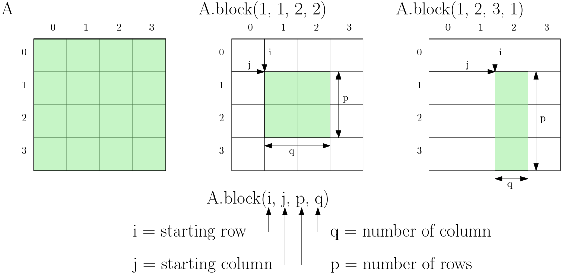
Here, we see the original matrix on the left. In the middle, I discard the first and last row and column, so I start row=1 and column=1, and I have two rows and columns. The example on the right shows a somewhat arbitrary example to help enforce the definitions of these different variables. We say that we start at row=1 and column=2, and we want to expand our view three rows down, with only a single column.
Remember, all of these views don't require memory allocation. Instead, what happens internally is that Eigen uses iterators to only serve the elements we have requested. Iterators are just pointers to data members and so don't store any memory themselves.
OK, with that, we should now be able to look at the next code example and see what is happening here. Try to see if you can make sense of the code, and I'll catch up with you afterwards.
#include <iostream>
#include <Eigen/Eigen>

int main() {
    // 2d structured grid parameters
    const auto numX = 5;
    const auto numY = 5;
    const auto numGP = 2; // number of ghost points

    // domain start and end
    const auto xStart = 0.0; const auto xEnd = 1.0;
    const auto yStart = 0.0; const auto yEnd = 1.0;

    // constant spacing
    const auto dx = (xEnd - xStart) / (numX - 1);
    const auto dy = (yEnd - yStart) / (numY - 1);

    // coordinate vectors
    auto Nx = numX + 2 * numGP;
    auto vectorStartX = xStart - numGP * dx;
    auto vectorEndX = xEnd + numGP * dx;
    Eigen::VectorXd x1D = Eigen::VectorXd::LinSpaced(Nx, vectorStartX, vectorEndX);

    auto Ny = numY + 2 * numGP;
    auto vectorStartY = yStart - numGP * dy;
    auto vectorEndY = yEnd + numGP * dy;
    Eigen::VectorXd y1D = Eigen::VectorXd::LinSpaced(Ny, vectorStartY, vectorEndY);

    // create 2d grid as matrix
    Eigen::MatrixXd x = x1D.replicate(1, Ny);
    Eigen::MatrixXd y = y1D.transpose().replicate(Nx, 1);

    // check x and y
    std::cout << "x:\n" << x << std::endl;
    std::cout << "\ny:\n" << y << std::endl;

    // create non-copy view into grid without ghost cells
    auto xNoGP = x.block(numGP, numGP, Nx - 2 * numGP, Ny - 2 * numGP);
    auto yNoGP = y.block(numGP, numGP, Nx - 2 * numGP, Ny - 2 * numGP);

    // check x and y
    std::cout << "\nxNoGP:\n" << xNoGP << std::endl;
    std::cout << "\nyNoGP:\n" << yNoGP << std::endl;

    // create non-copy view into internal mesh only
    auto xInt = x.block(numGP + 1, numGP + 1, Nx - 2 * numGP - 2, Ny - 2 * numGP - 2);
    auto yInt = y.block(numGP + 1, numGP + 1, Nx - 2 * numGP - 2, Ny - 2 * numGP - 2);

    // check x and y
    std::cout << "\nxInt:\n" << xInt << std::endl;
    std::cout << "\nyInt:\n" << yInt << std::endl;

    // create non-copy view into east and west boundary
    auto xEast = x.block(numGP + numX - 1, numGP, 1, Ny - 2 * numGP);
    auto yEast = y.block(numGP + numX - 1, numGP, 1, Ny - 2 * numGP);
    auto xWest = x.block(numGP, numGP, 1, Ny - 2 * numGP);
    auto yWest = y.block(numGP, numGP, 1, Ny - 2 * numGP);

    // check x and y
    std::cout << "\nxEast:\n" << xEast << std::endl;
    std::cout << "yEast:\n" << yEast << std::endl;
    std::cout << "xWest:\n" << xWest << std::endl;
    std::cout << "yWest:\n" << yWest << std::endl;

    // create solution vector to store a variable on the mesh
    Eigen::MatrixXd phi = Eigen::MatrixXd::Random(Nx, Ny);

    // create views into phi data at boundaries
    Eigen::Block<Eigen::MatrixXd> phiNorthBC = phi.block(numGP, Ny - numGP - 1, numX, 1);
    Eigen::Block<Eigen::MatrixXd> phiSouthBC = phi.block(numGP, numGP, numX, 1);
    Eigen::Block<Eigen::MatrixXd> phiEastBC = phi.block(Nx - numGP - 1, numGP, 1, numY);
    Eigen::Block<Eigen::MatrixXd> phiWestBC = phi.block(numGP, numGP, 1, numY);

    // set boundary conditions, phi=1 at north boundary, everything else to 0
    phiNorthBC.setConstant(1.0);
    phiSouthBC.setZero();
    phiEastBC.setZero();
    phiWestBC.setZero();

    // print out phi
    std::cout << "\nphi:\n" << phi << std::endl;

    // using blocks to compute the laplacian of phi
    auto i = numGP + 1;
    auto j = numGP + 1;
    auto sizeX = Nx - 2 * numGP - 2;
    auto sizeY = Ny - 2 * numGP - 2;
    auto dx2 = dx * dx;
    auto dy2 = dy * dy;

    Eigen::MatrixXd laplacian =
          phi.block(i + 1, j, sizeX, sizeY) / dx2
        - 2.0 * phi.block(i, j, sizeX, sizeY) / dx2
        + phi.block(i - 1, j, sizeX, sizeY) / dx2

        + phi.block(i, j + 1, sizeX, sizeY) / dy2
        - 2.0 * phi.block(i, j, sizeX, sizeY) / dy2
        + phi.block(i, j - 1, sizeX, sizeY) / dy2;

    // print out laplacian
    std::cout << "\nLaplacian:\n" << laplacian << std::endl;

    return 0;
}
This code produces the following output:
x:
 -0.5  -0.5  -0.5  -0.5  -0.5  -0.5  -0.5  -0.5  -0.5
-0.25 -0.25 -0.25 -0.25 -0.25 -0.25 -0.25 -0.25 -0.25
    0     0     0     0     0     0     0     0     0
 0.25  0.25  0.25  0.25  0.25  0.25  0.25  0.25  0.25
  0.5   0.5   0.5   0.5   0.5   0.5   0.5   0.5   0.5
 0.75  0.75  0.75  0.75  0.75  0.75  0.75  0.75  0.75
    1     1     1     1     1     1     1     1     1
 1.25  1.25  1.25  1.25  1.25  1.25  1.25  1.25  1.25
  1.5   1.5   1.5   1.5   1.5   1.5   1.5   1.5   1.5

y:
 -0.5 -0.25     0  0.25   0.5  0.75     1  1.25   1.5
 -0.5 -0.25     0  0.25   0.5  0.75     1  1.25   1.5
 -0.5 -0.25     0  0.25   0.5  0.75     1  1.25   1.5
 -0.5 -0.25     0  0.25   0.5  0.75     1  1.25   1.5
 -0.5 -0.25     0  0.25   0.5  0.75     1  1.25   1.5
 -0.5 -0.25     0  0.25   0.5  0.75     1  1.25   1.5
 -0.5 -0.25     0  0.25   0.5  0.75     1  1.25   1.5
 -0.5 -0.25     0  0.25   0.5  0.75     1  1.25   1.5
 -0.5 -0.25     0  0.25   0.5  0.75     1  1.25   1.5

xNoGP:
   0    0    0    0    0
0.25 0.25 0.25 0.25 0.25
 0.5  0.5  0.5  0.5  0.5
0.75 0.75 0.75 0.75 0.75
   1    1    1    1    1

yNoGP:
   0 0.25  0.5 0.75    1
   0 0.25  0.5 0.75    1
   0 0.25  0.5 0.75    1
   0 0.25  0.5 0.75    1
   0 0.25  0.5 0.75    1

xInt:
0.25 0.25 0.25
 0.5  0.5  0.5
0.75 0.75 0.75

yInt:
0.25  0.5 0.75
0.25  0.5 0.75
0.25  0.5 0.75

xEast:
1 1 1 1 1
yEast:
   0 0.25  0.5 0.75    1
xWest:
0 0 0 0 0
yWest:
   0 0.25  0.5 0.75    1

phi:
  0.680375    0.10794  -0.716795  -0.782382  -0.012834  -0.295083   0.780465    0.70184  -0.124725
 -0.211234 -0.0452059   0.213938   0.997849    0.94555   0.615449  -0.302214  -0.466669    0.86367
  0.566198   0.257742          0          0          0          0          0  0.0795207    0.86162
   0.59688  -0.270431          0  0.0258648   0.542715  -0.860489          1  -0.249586   0.441905
  0.823295  0.0268018          0   0.678224    0.05349   0.898654          1   0.520497  -0.431413
 -0.604897   0.904459          0    0.22528   0.539828  0.0519907          1  0.0250707   0.477069
 -0.329554    0.83239          0          0          0          0          0   0.335448   0.279958
  0.536459   0.271423  -0.198111   0.275105   0.783059  -0.615572   0.941268  0.0632129  -0.291903
 -0.444451   0.434594  -0.740419  0.0485744  -0.433371   0.326454   0.804416  -0.921439   0.375723

Laplacian:
 19.4316  -14.669  42.5039
 2.16125  42.3368 0.325243
18.5877 3.13285 38.8077There is quite a bit to go through, so let's go through this example together. We start by defining the number of points in the x and y direction using the numX and numYvariables on lines 6-7. These are the number of points that include the internal and boundary vertices, but not the ghost cells. Thus, we have 3 internal vertices and 2 vertices on each side. The number of ghost cells numGP is defined on line 8.
The total number of points, thus, in the x and y direction is numX + 2 numGP = 5 + 2 2 = 9 and numY + 2 numGP = 5 + 2 2 = 9, respectively. This is defined on lines 19 and 24 as Nx and Ny, respectively (well, perhaps not the best naming convention ... it has been a long day, bear with me).
We set the start and end location of the domain on lines 11 and 12. This is where we expect our boundary vertices to be located, not the first vertices (which are ghost cells, or rather, ghost vertices). That is, if we have 2 ghost cells, then we expect the third vertex to be on the boundary. If this is the x direction, then the third vertex should be at xStart = 0.0, as defined on line 11.
We compute the uniform spacing on lines 15-16 and call them dx and dy, as per common convention. On lines 20 and 21, we compute the location of the first and last vertex, that is, the location of the first and last ghost cell (vertex). This is for the x direction, and we repeat the same step on lines 25-26 for the y-direction.
Now that we have the total number of points (internal + boundary + ghost vertices), denoted by Nx and Ny, as well as the location of the first and last vertex in the x and y direction, we can use Eigen's LinSpaced function, which is defined for the vector class. This takes three arguments: the number of points, the start location, and the end location.
We call these new vectors x1D and y1D, as they are just one-dimensional vectors, but we want to now create a 2D grid from these. This is what we do on lines 30-31, where we replicate the x1D vector Ny times, while we replicate the y1D vector Nx times. In other words, take the x1D vector, interpret it as a column vector and then repeat it for Ny columns, giving us a [katex]Nx \times Ny[/katex] matrix. The same is true for the y1D vector, except that it is taken as a row vector and repeated for Nx rows.
Thus, for any index pair [katex]i,j[/katex], we can get the x and y coordinates now by indexing the x and y matrix, as defined on lines 30-31.
Now it is time to create some views. On lines 38 and 39, we create a view into the x and y matrix, where we are removing the ghost cells. Thus, these new matrices, which I have called xNoGP and yNoGP, have removed the first and last two vertices from the original matrix so that we are left with only boundary and internal vertices.
Let's look at line 38 in more detail. Here, we defined xNoGP as x.block(numGP, numGP, Nx - 2 numGP, Ny - 2 numGP). Remember, the first two entries are the offset into our original matrix. Since numGP is two in our example, our view starts at row 2 and column 2. Since C++ uses 0-based indexing, this means that row 0 and 1, as well as column 0 and 1, have been removed (as expected, since we have two ghost vertices).
We then have to specify how many rows and columns we want our view to span. I am simply removing the number of ghost cells from the total number here, but I could have also used numX and numY instead. Why didn't I do that? Well, I wrote those examples during the Christmas holiday, and no Christmas is complete without the looming possibility of at least stage 2 diabetes. Sober Tom in January is much more critical of himself than pre-Christmas Tom on a sugar rush ...
In any case, we apply the same logic on line 39 for the y coordinate. On lines 46-47, I do the same but now create a view onto internal vertices only. Thus, my new starting row and column becomes numGP + 1, while the last vertex becomes Nx - 2 * numGP - 2.
Remember, we do this because we may want to loop over only this particular data. In the case of the grid, there may not be a lot of use cases to do that (other than, perhaps, wanting to write out the solution for all the internal vertices, in this case, a view into the boundary and internal vertices may be advantageous). But for flow variables, this is definitely beneficial, and we get back to that in just a second.
Similarly, on lines 54-57, I create views to go over all vertices on the boundary, so that we can conveniently loop over all boundary vertices for the east, west, north, and south boundaries (though I show only east and west here, north and south are done similarly). Again, not very useful, but let's see an example where it would actually make sense to work with these views.
On line 66, I define a generic flow variable phi. It has the same [katex]Nx \times Ny[/katex] dimension as our x and y matrix, and it is initialised with random numbers. Similar to how I created views on lines 54-57 for the x and y matrix into the east and west boundary, we can create similar views for phi into the east, west, north, and south boundary, as seen on lines 69-72.
Then, on lines 75-78, I can now set the values to specific values as I wish, without having to loop over the matrix. Instead of the setConstant(value) function, I could have also used setOnes(), but the setConstant(value) method is more general, hence I have used it here.
OK, let's look at one more cool example of what you can achieve with blocks. I want to compute the Laplacian of phi on the internal domain. That is, I want to compute the second-order gradient. We have to do a bit of setup for this, which is shown on lines 84-89. Mainly, we define the start and end points in both x and y for our internal domain.
The starting row and column are numGP + 1, as defined by the i and j variable (and we will see in a second why I have chosen this particular name), and the last row and column in our domain are the sizeX and sizeY variable (stupendous naming). For convenience, I also define the square of dx ad dy as dx2 and dy2, respectively.
Now comes the magic! On lines 91-98, I define the Laplace operator and store the results in a Eigen::MatrixXd. I am using block() here again to generate views into my phi matrix. As a reminder, the Laplacian in 2D can be defined as:
\nabla^2 \phi = \frac{\partial^2 \phi}{\partial x^2} +\frac{\partial^2 \phi}{\partial y^2} \approx \frac{\phi_{i+1,j}-2\phi_{i,j}+\phi_{i-1,j}}{\Delta x^2} + \frac{\phi_{i,j+1}-2\phi_{i,j}+\phi_{i,j-1}}{\Delta y^2} \tag{12}Comparing that with lines 91-98, especially the i and j indices, we can see how our discretised equation naturally maps to the variables we define within the block() method. Why does this work? Well, we have defined i and j as the first row and column in our ```phi`` matrix that represents an internal vertex.
The vertex to the immediate left is at i-1, and appears in our discretised equation. If we now create a matrix with the same number of rows and columns (as specified by the third and forth argument to block(), which we can see is the same for all block() methods between lines 91-98), only shifted one entry to the left, then we get a matrix where all elements are shifted to the left by one element.
Thus, the first element in the matrix defined by block(i, j, ...) is at i=3, while the first element in block(i - 1, j, ...) is at i=2. Since both matrices have the same dimension, we can add and subtract them as we want. Thus, just by working with views (the block() method), we can create non-copy sub-matrices and use them to compute things on our matrix like gradients without having to write any loops. On top pf that, the generated code is rather expressive and required little documentation.
If you are coming from a Python world, and you use numpy and slicing, then this will feel very similar and, ineed, the core idea behind slicing numpy arrays and creating views into Eigen matrices using block() is the same.
Obviously, if we were to use a 3D grid now, we could no longer use Eigen in the same way. It is only defined for 2D matrices and does not natively extend to N-rank tensors. That makes sense; Eigen is supposed to be a linear algebra library, but at the same time, given the support for 1D vectors, it would be nice to see an extension to arbitrary tensors (and then, please, an experimental Deep Learning module ...).
In any case, I think we have now seen a good few examples of how we can use views and why we want to do that. In a nutshell, views allow us to declutter our code (removing for loops) and write more expressive instructions. These are two good reasons to consider using views when there is a chance to do so!
Interfacing Eigen with other data types
While I would be perfectly happy to accept Eigen as my only library of choice when it comes to writing my own CFD solvers, the truth is that as the complexity of our solver increases, so do the number of dependencies.
Let's consider the following scenario. We use Eigen to store our variables (velocity, pressure, temperature, etc.). At first, we implement an explicit solver and all is working well, until we extend the solver to handle turbulent flows through RANS modelling as well. With RANS support available, all of a sudden we get very small grid cells as dictated by the [katex]y^+[/katex] requirement.
In our previous CFL example, we saw that the time step is computed as:
\Delta t = \frac{CFL \Delta x}{u}\tag{13}Thus, as [katex]\Delta x[/katex] decreases, so does our time step [katex]\Delta t[/katex], since the maximum allowable CFL number will be around 1 for our explicit time integration. Now that we have to deal with painfully small time steps, we decide to implement an implicit time stepping, and so we need support for a linear system of equations solver.
We are in luck, Eigen does have support for that, and so we implement an implicit time stepping procedure, solve the linear system using Eigen, and can support larger time steps now (we will look at Eigen's support for linear systems as well). But, after some point, we want to simulate even larger systems and realise that we need parallel computing.
Eigen does not support parallelisation, and so we are forced to change to a different linear system of equation solver, like PETSc (which we will also cover in this series eventually ... If you are from the future, then it may already be available, lucky you!). However, all of our internal data types assume that we are using Eigen to store our data, so do we have to change our underlying data structure?
No! Eigen was and still is developed by forward-thinking individuals who have already anticipated your need to take your data out of the Eigen ecosphere and dump it into another library. And this is rather simple to do, as we will see shortly.
By the way, Eigen is just following the standard C++ approach here. The entire standard template library (STL) was designed with interoperability in mind. You can always extract the raw data out of a, say, std::vector, and place it inside another object that expects a raw pointer. That is the secret ingredient, under the hood, be it a std::vector or a Eigen::Matrix, data is just stored as a plain C-style array.
In the STL, we can get this raw pointer by calling the data() method on an object like std::vector, and Eigen follows this convention. That is, call data() on an Eigen object like a matrix or vector, and you get the underlying raw pointer. You can use that to pass that now to other libraries.
Equally, Eigen has support to read in raw C-style pointers and map them to native Eigen types. Eigen uses the Eigen::Map type for exactly this purpose. It takes one template argument, which is the type that we want to convert the raw pointer to. We will see this in the next example, so have a look through it first, and then we discuss the code below again.
#include <iostream>
#include <Eigen/Eigen>
#include <vector>

int main() {
    // create a std::vector with 9 entries
    std::vector<double> vec = {1.0, 2.0, 3.0, 4.0, 5.0, 6.0, 7.0, 8.0, 9.0};

    // convert to Eigen vector through Eigen::Map
    Eigen::Map<Eigen::VectorXd> eigen_vec(vec.data(), vec.size());

    // or, create 3 by 3 matrix directly
    Eigen::Map<Eigen::MatrixXd> eigen_mat(vec.data(), 3, 3);

    // print the Eigen vectors and matrices
    std::cout << "Eigen vector:\n" << eigen_vec.transpose() << std::endl;
    std::cout << "\nEigen matrix (not expected order?!):\n" << eigen_mat << std::endl;

    // specify storage order of matrix explicitly, requires full template parameters
    Eigen::Map<Eigen::Matrix<double, Eigen::Dynamic, Eigen::Dynamic, Eigen::RowMajor>> eigen_mat2(vec.data(), 3, 3);
    std::cout << "\nEigen matrix (expected order):\n" << eigen_mat2 << std::endl;

    // let's make sure no data was copied by comparing storage addresses
    std::cout << "\nstd::vector  address: " << &vec[0] << std::endl;
    std::cout << "Eigen vector address: " << &eigen_vec(0) << std::endl;
    std::cout << "Eigen matrix address: " << &eigen_mat(0,0) << std::endl;

    // modifying Eigen will modify std::vector
    eigen_vec(0) = 10.0;
    eigen_mat(1,1) = 20.0;
    eigen_mat2(2,2) = 30.0;

    std::cout << "\nstd::vector:  ";
    for (const auto& v : vec) std::cout << v << " ";
    std::cout << std::endl;

    std::cout << "Eigen vector: " << eigen_vec.transpose() << std::endl;
    std::cout << "\nEigen matrix:\n" << eigen_mat << std::endl;
    std::cout << "\nEigen matrix:\n" << eigen_mat2 << std::endl;

    return 0;
}This code produces the following output:
Eigen vector:
1 2 3 4 5 6 7 8 9

Eigen matrix (not expected order?!):
1 4 7
2 5 8
3 6 9

Eigen matrix (expected order):
1 2 3
4 5 6
7 8 9

std::vector  address: 0x15612b0
Eigen vector address: 0x15612b0
Eigen matrix address: 0x15612b0

std::vector:  10 2 3 4 20 6 7 8 30
Eigen vector: 10  2  3  4 20  6  7  8 30

Eigen matrix:
10  4  7
 2 20  8
 3  6 30

Eigen matrix:
10  2  3
 4 20  6
7 8 30On line 7, I am just defining and initialising a std::vector containing 9 elements. On line 10, I am converting the std::vector to an Eigen::VectorXd using the Eigen::Map class. We can see that the template parameter to Eigen::Map is Eigen::VectorXd, that is, the type we want to convert to. We store the results in the variable eigen_vec.
We can see that the arguments we pass to the constructor of Eigen::Map are the raw pointer (in this case, exposed by calling vec.data() on the std::vector object), as well as the number of elements pointed to by the raw pointer (which we get by calling vec.size()). This provides us with a 1D vector; however, we can also use Eigen::Map to create a matrix object as seen on line 13, where we have to now give the number of rows and columns to the constructor.
When we print out the matrix on line 17, we may notice that the matrix is not in the order we would expect it to be. That is, the first row is 1, 4, 7, followed by 2, 5, 8, followed by 3, 6, 9. We may have wished to create the matrix containing the following rows instead: 1, 2, 3, 4, 5, 6, and 7, 8, 9.
Since Eigen stores matrices in column-major order (meaning we fill the matrix column-by-column, not row-by-row), this is the default behaviour. If we wanted to store the matrix in row-major order, we would need to specify that as a template parameter to the matrix type. This is what we can see on line 20. We have to provide the required first three template parameters (the type, and number of rows and columns, which in this case is set to dynamic so it can be inferred at runtime), but I am also setting the fourth template parameter here.
This parameter is simply Eigen::RowMajor, and tells Eigen to store the data in exactly that way. The default is Eigen::ColumnMajor, so if that is what we want, or are happy with, there is no need for us to define all template parameters. Printing this matrix now on line 21 shows the matrix created in a row-by-row fashion.
On lines 24-26, I am printing the address of the original std::vector and the vector and matrix created in Eigen using Eigen::Map. Since we are dealing with a raw pointer here, we haven't passed around any data, but only the address of where to find that data. Therefore, all are pointing to the same address (data), and so modifying one of these new objects will also modify the original std::vector.
This is exactly what we do on lines 29-31. Here, we modify both the vector and matrix created in Eigen. Afterwards, we print the content of the original std::vector, which has now changed, since it points to the same data as the Eigen arrays. I also print there the created Eigen objects for convenience to see that all objects have the same data.
We didn't actually look at any raw pointers in the code example above; they were all hidden behind the data() method. But just for completeness, let's also look at raw pointers explicitly. The following example shows how we can create a raw pointer in C++ and then pass that to Eigen using the Eigen::Map class:
// use raw pointer instead
int vecSize = 9;
double *vec = new double[vecSize]{1.0, 2.0, 3.0, 4.0, 5.0, 6.0, 7.0, 8.0, 9.0};

// convert to Eigen vector through Eigen::Map
Eigen::Map<Eigen::VectorXd> eigen_vec(vec, vecSize);We can also go the other way around, i.e. getting a raw pointer from an Eigen matrix or vector:
// create Eigen vector
Eigen::Vector3d vecEigen = Eigen::Vector3d::Random();

// convert Eigen vector to raw pointer
double *vecRaw = new double[3];
vecRaw = vecEigen.data();As you can see, you will never be locked-in to use Eigen beyond what you need it for; it will always allow you to interact and flirt with other libraries to live the polygamy lifestyle you crave.
Computing gradients on unstructured grids using the least-squares and related approaches
Two examples ago, I showed you how you can compute the Laplacian, i.e. the second-order derivative (diffusion term) on a 2D structured grid. In this example, I want to expand on this and look at how we can compute gradients, in general, on an arbitrary 2D (or even 3D) grid.
Consider the following cell arrangement:

Here, we have 5 cells given to us. These are all quad elements, but they could be really anything; the shape doesn't matter. What matters it the location of the centroids, that is, [katex]p_0[/katex] to [katex]p_4[/katex], as well as the values stored at the centroid, as indicated by [katex]\phi_0[/katex] to [katex]\phi_4[/katex]. Here, [katex]\phi[/katex] is a generic placeholder again, and could stand for the velocity, density, pressure, temperature, etc.
Now let's make it more real. Let's say we are solving an incompressible flow, and we are using some pressure projection method (e.g. Chorin's exact projection or an inferior approach like the SIMPLE or PISO algorithm). In this method, we obtain a Poisson equation for the pressure field, which has the following form:
\nabla^2 p = S
\tag{14}
Here, [katex]S[/katex] is the source term, which for both exact and approximate (SIMPLE, PISO) projection methods is fairly similar. It has the form of:
S=a\nabla\cdot \mathbf{u}\tag{15}where the only difference is in the choice of [katex]a[/katex]. For Chorin's exact project method, we have: [katex]a=\rho/\Delta t[/katex], and for SIMPLE, PISO, etc., it is the main diagonal of the coefficient matrix from the momentum equation (which also contains the term [katex]\rho/\Delta t[/katex], plus a few additional terms we have to introduce because we decided to butcher the Navier-Stokes equations).
If you want to see how to derive this pressure Poisson equation for the exact and approximate pressure projection methods, you can find all the details in my article on incompressible flows.
Let's discretise Eq.(14) using a finite volume method. For that, we need to first expand the equation into a scalar representation. Given that the example shown in the figure above is 2D, let's expand the pressure Poisson equation into 2D:
\nabla^2 p = \frac{\partial^2 p}{\partial x^2} + \frac{\partial^2 p}{\partial y} = S
\tag{16}
Next, we integrate over a finite volume (which is the same as the volume of our cell), and we get:
\int_V \frac{\partial^2 p}{\partial x^2} \mathrm{d}V + \int_V \frac{\partial^2 p}{\partial y^2} \mathrm{d}V= \int_V S\mathrm{d}V\tag{17}We now apply the Gauss theorem, which turns our volume integral into a integral. We do that because surface integrals are conservative, volume integrals are not. Given that the pressure Poisson equation is derived from the conservation of mass (continuity equation), a conservative discretisation is preferred. If you want a more thorough discussion on that, refer to my write-up on why surface integrals are preferred.
After we apply the Gauss theorem, we end up with the following term:
\int_A \vec{n}\cdot\frac{\partial p}{\partial x}\mathrm{d}A + \int_A \vec{n}\cdot\frac{\partial p}{\partial y}\mathrm{d}A= S
\tag{18}
To see how we end up with this term, you may wish to look at my finite volume discretisation of second-order derivatives write-up. However, as you can see, we end up with the need to evaluate the first-order gradients [katex]\partial p/\partial x[/katex] and [katex]\partial p/\partial y[/katex], and in the following, this is exactly what we will be computing on an arbitrary unstructured grid (the same works, of course, also for structured grids).
This is known in the CFD literature as the least-square gradient computation, and it is something you will find in any major CFD solver.
Let's return to the figure above. Here, you can mentally replace [katex]\phi[/katex] with the pressure [katex]p[/katex]. To compute the gradients of the pressure in the [katex]x[/katex] and [katex]y[/katex] direction, we start with the total differential of the pressure.
Let's look at the total differential in 2D. We can write this in a general form as:
\mathrm{d}f = \frac{\partial f}{\partial x}\mathrm{d}x + \frac{\partial f}{\partial y}\mathrm{d}y\tag{19}Consider an air-conditioning unit. In order to cool down a room, you can change two settings: the temperature of the air coming out from the air conditioning unit, as well as the fan speed at which air is being blown out of the unit. Let's say that the temperature is denoted by [katex]T[/katex] and the fan speed by [katex]s[/katex], then, we can write the total differential for the cooling rate [katex]f[/katex] of our room as:
\mathrm{d}f = \frac{\partial f}{\partial T}\mathrm{d}T + \frac{\partial f}{\partial s}\mathrm{d}s\tag{20}No changes in the temperature or fan speed settings mean [katex]\mathrm{d}T=\mathrm{d}s=0[/katex], and thus, [katex]\mathrm{d}f=0[/katex]. No change in room cooling is observed. The partial derivatives [katex]\partial f/\partial T[/katex] and [katex]\partial f/\partial s[/katex] determine how strongly the cooling rate [katex]f[/katex] is affected by changes in the temperature and fan speed. We can view them simply as scaling factors.
Let's bring that back to our pressure. We can write the total differential for the pressure as:
\mathrm{d}p = \frac{\partial p}{\partial x}\mathrm{d}x + \frac{\partial p}{\partial y}\mathrm{d}y
\tag{21}
Eq.(21) tells us how the pressure field changes as we move freely in the [katex]x[/katex] and [katex]y[/katex] space. No movement in [katex]x[/katex] and [katex]y[/katex], i.e. [katex]\mathrm{d}x = \mathrm{d}y = 0[/katex] means no change in pressure either, that is, [katex]\mathrm{d}p=0[/katex].
Looking at Eq.(21), we can make the following observations:
- It already contains the first-order pressure gradients with respect to the [katex]x[/katex] and [katex]y[/katex] directions that we want to compute, and
- All other quantities are properties we can compute from the mesh and the pressure field directly.
For example, the pressure difference [katex]\mathrm{d}p[/katex] really just is the difference in pressure between two centroids. For example, we can write the pressure difference between cell 0 and 1 as [katex]\mathrm{d}p = p_1 - p_0[/katex]. Looking at the figure above, we already have values for [katex]\phi_0=p_0[/katex] and [katex]\phi_1=p[/katex] given, so we can compute this directly as [katex]\mathrm{d}p = p_1 - p_0 = 0.3 - 0.7 = -0.4[/katex].
Both [katex]\mathrm{d}x[/katex] and [katex]\mathrm{d}y[/katex] represent the distance in the [katex]x[/katex] and [katex]y[/katex] space between two points where we are measuring the pressure difference. We have established that we want to compute the difference in pressure between cell centroids 0 and 1, and we have already obtained [katex]\mathrm{d}p[/katex]. Now, we can simply look at the distance between both centroids and write it for the [katex]x[/katex] and [katex]y[/katex] directions separately.
In the [katex]x[/katex] direction, we have [katex]\mathrm{d}x=\Delta x = x_1 - x_0 = 3.375 - 2.0 = 1.375[/katex]. In the [katex]y[/katex] direction, we have [katex]\mathrm{d}y=\Delta y = y_1 - y_0 = 2.0 - 2.0 = 0.0[/katex]. Thus, returning to Eq.(21), we can see that [katex]\partial p /\partial x[/katex] and [katex]\partial p/\partial y[/katex] are unknown, while [katex]\mathrm{d}p[/katex], [katex]\mathrm{d}x[/katex], and [katex]\mathrm{d} y[/katex] can be computed from the mesh and the flow field.
I have only shown how to compute [katex]\mathrm{d}p[/katex], [katex]\mathrm{d}x[/katex], and [katex]\mathrm{d} y[/katex] for cell 1; however, we can also perform the same computation for cells 2, 3, and 4. Instead of writing Eq.(21) as it is, we can also express it in vector form for all faces as:
\begin{bmatrix}
p_1 - p_0 \\
p_2 - p_0 \\
p_3 - p_0 \\
p_4 - p_0
\end{bmatrix}=
\frac{\partial p}{\partial x}
\begin{bmatrix}
x_1 - x_0 \\
x_2 - x_0 \\
x_3 - x_0 \\
x_4 - x_0
\end{bmatrix} +
\frac{\partial p}{\partial y}
\begin{bmatrix}
y_1 - y_0 \\
y_2 - y_0 \\
y_3 - y_0 \\
y_4 - y_0
\end{bmatrix}\tag{22}
We can further combine both the pressure gradients and the distances in the [katex]x[/katex] and [katex]y[/katex] directions to make this a fully matrix-based operation. We obtain:
\begin{bmatrix}
p_1 - p_0 \\
p_2 - p_0 \\
p_3 - p_0 \\
p_4 - p_0
\end{bmatrix}=
\begin{bmatrix}
x_1 - x_0 & y_1 - y_0 \\
x_2 - x_0 & y_2 - y_0 \\
x_3 - x_0 & y_3 - y_0 \\
x_4 - x_0 & y_4 - y_0
\end{bmatrix}
\begin{bmatrix}
\frac{\partial p}{\partial x} \\[1em]
\frac{\partial p}{\partial y}
\end{bmatrix}\tag{23}
Let's clean up the notation a bit and introduce [katex]\Delta_i \phi = \phi_i - \phi_0[/katex], with [katex]\phi[/katex] being either the pressure [katex]p[/katex], the [katex]x[/katex] or [katex]y[/katex] coordinate. This results in the more compact form of:
\begin{bmatrix}
\Delta p_1 \\
\Delta p_2 \\
\Delta p_3 \\
\Delta p_4
\end{bmatrix}=
\begin{bmatrix}
\Delta x_1 & \Delta y_1 \\
\Delta x_2 & \Delta y_2 \\
\Delta x_3 & \Delta y_3 \\
\Delta x_4 & \Delta y_4
\end{bmatrix}
\begin{bmatrix}
\frac{\partial p}{\partial x} \\[1em]
\frac{\partial p}{\partial y}
\end{bmatrix}\tag{24}
Swapping the left and right-hand side results in:
\underbrace{
\begin{bmatrix}
\Delta x_1 & \Delta y_1 \\
\Delta x_2 & \Delta y_2 \\
\Delta x_3 & \Delta y_3 \\
\Delta x_4 & \Delta y_4
\end{bmatrix}}_A
\underbrace{
\begin{bmatrix}
\frac{\partial p}{\partial x} \\[1em]
\frac{\partial p}{\partial y}
\end{bmatrix}}_x =
\underbrace{
\begin{bmatrix}
\Delta p_1 \\
\Delta p_2 \\
\Delta p_3 \\
\Delta p_4
\end{bmatrix}}_b
\tag{25}
We can further simplify that into symbolic notation as [katex]\mathbf{Ax}=\mathbf{b}[/katex]. Now, the eagle-eyed amongst you will have noted that Eq.(25) contains 2 unknowns (the pressure gradient terms) for 4 equations. The system is over-determined, or over-constrained.
In such cases, we can resort to the least-squares problem, which will give us a best fit through an overdetermined system; that is, in this case, we can compute the best fit for the pressure gradient over all cell pairs.
To do that, let's use the symbolic notation of [katex]\mathbf{Ax}=\mathbf{b}[/katex]. We want to compute [katex]\mathbf{x}[/katex], which is our pressure gradient. Since [katex]\mathbf{A}[/katex] is of the same size as the number of faces within a given cell, it is a small matrix and so our immediate thought may be to compute the inverse and then multiply that to the right so that we get [katex]\mathbf{x}=\mathbf{A}^{-1}\mathbf{b}[/katex].
However, we cannot do that, because [katex]\mathbf{A}[/katex] has dimensions of [katex](nFaces,\,D)[/katex], where [katex]D[/katex] is the dimension of the problem (in our case [katex]D=2[/katex] for a 2D problem). In 2D, there are no elements that have only 2 faces, and in 3D, there are no elements that have only 3 faces. [katex]\mathbf{A}[/katex] can never be a square matrix, and so we cannot invert it.
However, now let's consider the product of a matrix with itself; specifically, it's transpose. Let's look at the result of [katex]\mathbf{A}^T\mathbf{A}[/katex]. In our example, we have a 4-by-2 matrix, so let's see how this would be computed:
\mathbf{A}^T\mathbf{A}=
\begin{bmatrix}
a_1 & a_2 & a_3 & a_4 \\
a_5 & a_6 & a_7 & a_8
\end{bmatrix}
\begin{bmatrix}
b_1 & b_2 \\
b_3 & b_4 \\
b_5 & b_6 \\
b_7 & b_8
\end{bmatrix}=\\[1em]
\begin{bmatrix}
(a_1b_1 + a_2b_3 + a_3b_5 + a_4b_7)  & (a_1b_2 + a_2b_4 + a_3b_6 + a_4b_8) \\
(a_5b_1 + a_6b_3 + a_7b_5 + a_8b_7)  & (a_5b_2 + a_6b_4 + a_7b_6 + a_8b_8)
\end{bmatrix}\tag{26}
Lo and Behold, applying the transpose to our matrix [katex]\mathbf{A}[/katex] has turned our non-square matrix into a square matrix. In fact, our [katex](nFaces,\,D)[/katex] sized matrix has turned into a [katex](D,\,D)[/katex] sized matrix (in our case, with [katex]D=2[/katex], we have a [katex](2,\,2)[/katex] matrix, which is easily and cheaply inverted). Hallelujah, we can compute its inverse again and then place it on the right-hand side. Thus, writing the inverse of [katex]\mathbf{A}[/katex], that is, [katex]\mathbf{A}^{-1}[/katex] on the right-hand side, we obtain:
\mathbf{Ax}=\mathbf{b} \\[1em]
\mathbf{A}^T\mathbf{Ax}=\mathbf{A}^T\mathbf{b} \\[1em]
\mathbf{x} = (\mathbf{A}^T\mathbf{A})^{-1}\mathbf{A}^T\mathbf{b}
\tag{27}
Remember, [katex]\mathbf{x}[/katex] in this case is the vector containing our pressure gradient, that is, [katex]\mathbf{x}=(\partial p/\partial x,\,\partial p/\partial y)^T[/katex]. Eq.(27) is also referred to as the normal equation in the context least-square problems. We now have an equation to solve, and a need to use a linear algebra package to do so. What a coincidence, we can use Eigen for exactly that purpose!
Let's define an arbitrary function for our pressure variable [katex]p[/katex]. We do that so that we can analytically compute the pressure gradient, which we can use to check whether our implementation is correct or not. Let's assume our pressure follows the following function:
p(x, y) = \frac{1}{2}x^2 - 0.1 y^2\tag{28}With this arbitrary function defined, we can compute the derivatives in the [katex]x[/katex] and [katex]y[/katex] direction directly as:
\frac{\partial p}{\partial x} = x \\[1em]
\frac{\partial p}{\partial y} = 0.3y^2\tag{29}
Thus, let's summarise the data for the pressure. The following table shows the pressure value and its derivative with respect to [katex]x[/katex] and [katex]y[/katex] at the various centroids, as seen at the beginning of this section.
| Cell ID | x-coordinate | y-coordinate | |||
|---|---|---|---|---|---|
| 0 | 2 | 2 | 1.60 | 2.00 | -0.40 |
| 1 | 3.375 | 2 | 5.30 | 3.38 | -0.40 |
| 2 | 2 | 0.625 | 1.96 | 2.00 | -0.13 |
| 3 | 0.625 | 1.75 | -0.11 | 0.63 | -0.35 |
| 4 | 3.375 | 3.375 | 0.86 | 2.00 | -0.68 |
Since we are interested in computing the gradient for cell ID 0, we expect our least-square code to compute gradients of [katex](2.0,\,-0.4)^T[/katex] for this cell. The following code defines a Gradient class that will compute the gradient using various built-in methods into Eigen, as well as our least-square approach as seen in Eq.(27). Have a look through the code, and as usual, we'll discuss the code below together.
#include <iostream>
#include <Eigen/Eigen>

class Gradient {
public:
    using VectorType = typename Eigen::Matrix<double, Eigen::Dynamic, 1>;
    using MatrixType = typename Eigen::Matrix<double, Eigen::Dynamic, 2>;

public:
    Gradient(const VectorType &dx, const VectorType &dy) {
        _A.resize(dx.rows(), 2);
        _A.col(0) = dx;
        _A.col(1) = dy;
    }

    // Least-squares method
    VectorType leastSquares(const VectorType &phiDifferences) const {
        MatrixType ATA = _A.transpose() * _A;
        VectorType ATb = _A.transpose() * phiDifferences;
        return ATA.inverse() * ATb;
    }

    // Cholesky decomposition
    VectorType cholesky(const VectorType &phiDifferences) const {
        MatrixType ATA = _A.transpose() * _A;
        VectorType ATb = _A.transpose() * phiDifferences;
        return ATA.ldlt().solve(ATb);
    }

    // LU decomposition
    VectorType lu(const VectorType &phiDifferences) const {
        MatrixType ATA = _A.transpose() * _A;
        VectorType ATb = _A.transpose() * phiDifferences;
        return ATA.partialPivLu().solve(ATb);
    }

    // QR decomposition
    VectorType qr(const VectorType &phiDifferences) const {
        return _A.colPivHouseholderQr().solve(phiDifferences);
    }

    // Single-value decomposition reconstruction
    VectorType svd(const VectorType &phiDifferences) const {
        return _A.bdcSvd(Eigen::ComputeThinU | Eigen::ComputeThinV).solve(phiDifferences);
    }

private:
    MatrixType _A;
};

int main() {
    // difference between phi at the cell centroid and its neighbours
    Gradient::VectorType phi(4);
    phi << 5.3 - 1.6, 1.96 - 1.6, -0.11 - 1.6, 0.86 - 1.6;

    // delta x vector
    Gradient::VectorType dx(4);
    dx << 1.375, 0.0, -1.375, 0.0;

    // delta y vector
    Gradient::VectorType dy(4);
    dy << 0.0, -1.375, -0.25, 1.375;

    // compute least squares gradient
    Gradient grad(dx, dy);

    std::cout << "Least squares gradient: (" << grad.leastSquares(phi).transpose() << ")" << std::endl;
    std::cout << "LU       decomposition: (" << grad.lu(phi).transpose() << ")" << std::endl;
    std::cout << "Cholesky decomposition: (" << grad.cholesky(phi).transpose() << ")" << std::endl;
    std::cout << "QR       decomposition: (" << grad.qr(phi).transpose() << ")" << std::endl;
    std::cout << "SVD      decomposition: (" << grad.svd(phi).transpose() << ")" << std::endl;

    return 0;
}This produces the following output:
Least squares gradient: (  2.00927 -0.461967)
LU       decomposition: (  2.00927 -0.461967)
Cholesky decomposition: (  2.00927 -0.461967)
QR       decomposition: (  2.00927 -0.461967)
SVD decomposition: ( 2.00927 -0.461967)First of all, we can see that all methods produce a gradient for cell ID 0 that closely matches our expected exact gradient of [katex](2.0,\,-0.4)^T[/katex]. It isn't exact, but such is the nature of numerical modelling. I assume a quadratic relationship here for the pressure; if you try even higher orders, e.g. cubic relationships for the pressure, for example, this difference will only get larger.
We can try to define smaller cells (and thus make [katex]\Delta x[/katex] and [katex]\Delta y[/katex] go closer to zero), and if we do, we will observe that our gradient will also become a closer approximation based on the exact value.
You may ask why I bothered to show you so many different ways of computing the gradient, especially as all of their values are, in this case anyways, identical. Well, again, we are dealing with numerical computation here, and some methods are more robust than others. For example, once we start to add poor-quality metrics to the mix, we start to see differences in the methods.
The order in which I have implemented and printed the result to the screen is from the least to the most computationally expensive method. However, as we go from least squares to single-value decomposition (SVD), we also gain stability. So, on unstructured grids with highly skewed cells, for example, I would check which of these methods provides me with the best trade-off between robustness, speed, and accuracy. If in doubt, the QR decomposition is a commonly used one. You have my blessing to use it!
But, to make an informed decision, have a look at Eigen's benchmark of these different decomposition techniques. You can see that Cholesky and LU decompositions are very fast, and typically at least one order of magnitude faster than the singular-value decomposition (SVD).
Looking at the code now, we can see that our gradient class is defined on lines 4-49. The first thing I do (and I commonly like to do for documentation purposes) is to define meaningful and descriptive typedefs (custom variable names) that are intention-revealing. This is done on lines 6-7, which are made public (line 5), meaning that if I ever needed to access this type outside this class, I could.
For example, we pass in the precomputed distances to the constructor on line 10, which are all of type VectorType. This means I will need to construct this outside of my class. As can be seen in my main function between lines 51-75, I use this type on lines 53, 57, and 61 to define vectors that I pass to the Gradient class. I can access these new typedefs with the Class::Type syntax, where I have to specify the class name (e.g. Gradient) and the type I want to use from this class (e.g. VectorType).
If I don't make my typedefs public, then I cannot use them this way. As a rule of thumb, if I need the typedefs outside my class, make it public, otherwise if it is just for internal class documentation purposes, make it private or protected, if your class uses inheritance.
Within the constructor, I first resize the matrix to the correct size, based on the number of rows within the dx vector (I could have also used the dy vector here). The number of rows here corresponds to the number of faces for the current cell for which I am trying to compute the gradient. Thus, if I had a grid with different elements, my _A matrix may have a different number of rows for each cell.
On lines 12 and 13, I simply set the first and second column to the values of dx and dy, which essentially gives me:
A=
\begin{bmatrix}
\Delta x_1 & \Delta y_1 \\
\Delta x_2 & \Delta y_2 \\
\Delta x_3 & \Delta y_3 \\
\Delta x_4 & \Delta y_4
\end{bmatrix}\tag{30}
Return to Eq.(27), we had:
\mathbf{x} = (\underbrace{\mathbf{A}^T\mathbf{A}}_{ATA})^{-1}\underbrace{\mathbf{A}^T\mathbf{b}}_{ATb}\tag{31}Here, using the variable definitions ATA and ATb, we can see how this equation is implemented on lines 18-20 for the least-square approach. If we now look through the various other methods, we see, for example, that the Cholesky and LU decomposition follow a very similar pattern, i.e. see lines 24-28 and 31-35, respectively.
Using either the QR decomposition or single-value decomposition (SVD) on lines 38-40 and 43-45, respectively, we see that we can operate directly on our coefficient matrix _A and the difference vector of our pressure, no need to first compute the transpose and inverse of the matrix.
For the SVD example, you see that we pass these odd looking variables to the bdcSvd() function, which are Eigen::ComputeThinU and Eigen::ComputeThinV. This is specific to SVD and, I thought of diving into this here and showing another cool example you can use Eigen for (reduced order modelling, where SVD plays a critical role), but that example exploded quickly, and it is probably best to save that for a later article.
Without going into the details here, let's just say that using both the Eigen::ComputeThinU and Eigen::ComputeThinV flags will save computational cost, and, we really want to do that as SVD is already rather expensive. As alluded to previously, SVD can easily be an order of magnitude slower than, say, the Cholesky decomposition, and reducing computational cost is probably something we are interested in!
However, I should also state for balance that unless our mesh is moving, we only need to compute the inverse or other operations performed on _A once. This is the call to bcdSvd(). This is expensive, so we could also call this function for each cell once, store the results, and then, during each time step when we need to compute gradients, we would call the solve() function on these precomputed variables.
If the mesh is changing, so will our distances between centroids, and so there is no way for us to store these values. If you are into fluid-structure interactions, I'm afraid this isn't for you.
Before I close this section, let us return briefly to Eq.(18), which was given as:
\int_A \vec{n}\cdot\frac{\partial p}{\partial x}\mathrm{d}A + \int_A \vec{n}\cdot\frac{\partial p}{\partial y}\mathrm{d}A= S\tag{32}Let's finish the discretisation. In the finite-volume method, we replace the surface integrals by summations over all faces that make up a given cell, and so we could write this equation as:
\sum_{i=0}^{nFaces} \vec{n}_i\cdot\frac{\partial p}{\partial x}\bigg|_i A_i + \sum_{i=0}^{nFaces} \vec{n}_i\cdot\frac{\partial p}{\partial y}\bigg|_i A_i= S\tag{33}We have already obtained the pressure gradient, albeit at cell centroids. If we want to have this at the cell faces, we can linearly interpolate them between cell centroids. We are only missing the normal vector and the area of the face. We can compute these from the vertices of the face.
For example, consider the vertices that make up the face between the cells with centroid ID 0 and 1. We have two vertices that are defined as [katex]v_1=(2.75,\,1.25)^T[/katex] and [katex]v_2=(3.0,\,3.0)^T[/katex]. The normal vector, in 2D, can be computed as:
\vec{n}=\frac{1}{\text{mag}(n)}
\begin{bmatrix}
-(v_{2,y} - v_{1,y}) \\
(v_{2,x} - v_{1,x})
\end{bmatrix}\tag{34}
The magnitude is defined as:
\text{mag}(n) = \sqrt{n_x^2 + n_y^2}\tag{35}The area can be computed as:
A=\sqrt{(v_{2,x}-v_{1,x})^2 + (v_{2,y}-v_{1,y})^2}\tag{36}If we wanted to apply that to our example, then we could compute the normal vector (not yet normalised) as:
\vec{n}=\frac{1}{\text{mag}(n)}
\begin{bmatrix}
-(3.0 - 1.25) \\
(3.0 - 2.75)
\end{bmatrix}=\frac{1}{\text{mag}(n)}
\begin{bmatrix}
-1.75 \\
0.25
\end{bmatrix}\tag{37}
The magnitude of the normal vector can be computed as:
\text{mag}(n) = \sqrt{(-1.75)^2 + 0.25^2} \approx 1.77\tag{38}Therefore, the normalised normal vector becomes:
\vec{n}=
\begin{bmatrix}
-0.98 \\
0.14
\end{bmatrix}\tag{39}
Finally, the area for the face becomes:
A=\sqrt{(3.0-2.75)^2 + (3.0-1.25)^2}=\sqrt{0.25^2+1.75^2} \approx 1.77 \tag{40}With that, we have all quantities we need, and we can compute the left-hand side (at least for the first cell) of our pressure Poisson solver. To be clear, let's write this out. We have:
\sum_{i=0}^{nFaces} \vec{n}_i\cdot\frac{\partial p}{\partial x}\bigg|_i A_i + \sum_{i=0}^{nFaces} \vec{n}_i\cdot\frac{\partial p}{\partial y}\bigg|_i A_i= S\\[1em]
\left(\vec{n}_1\cdot\frac{\partial p}{\partial x}\bigg|_1 A_1 + \vec{n}_2\cdot\frac{\partial p}{\partial x}\bigg|_2 A_2 + \vec{n}_3\cdot\frac{\partial p}{\partial x}\bigg|_3 A_3 + \vec{n}_4\cdot\frac{\partial p}{\partial x}\bigg|_4 A_4\right) +\\[1em]
\left(\vec{n}_1\cdot\frac{\partial p}{\partial y}\bigg|_1 A_1 + \vec{n}_2\cdot\frac{\partial p}{\partial y}\bigg|_2 A_2 + \vec{n}_3\cdot\frac{\partial p}{\partial y}\bigg|_3 A_3 + \vec{n}_4\cdot\frac{\partial p}{\partial y}\bigg|_4 A_4\right) = S\\[1em]\tag{41}
For our first cell, we have just computed [katex]\vec{n}_1=(-0.98,\,0.14)^T[/katex] and [katex]A_1=1.77[/katex], we need the pressure gradient at face 1. Let's use a simple linear interpolation:
\frac{\partial p}{\partial x}\bigg|_1 = \frac{1}{2}\frac{\partial p}{\partial x}\bigg|_{cell\, 0} + \frac{1}{2}\frac{\partial p}{\partial x}\bigg|_{cell\, 1}\tag{42}For the moment, we have only computed the gradient for cell 0. In reality, we would compute the gradients for each cell and store them in an array. After we have done this, we can then interpolate gradients to the face centroids and proceed.
Now, you have seen me do this for cell 0; the steps involved to compute the gradient for cell 1 are going to be exactly the same, with just different values for [katex]p[/katex], [katex]\Delta x[/katex], and [katex]\Delta y[/katex].
Instead of redoing all of this, let's be lazy and compute the gradient for cell 1 using the analytic solution instead. The gradient would be slightly different using, for example, our least-square approach (or, for that matter, any of the other methods), but it'll do for this example.
The pressure gradient for cell 1, using the analytic solution, is [katex]\partial p/\partial x=3.375[/katex] and [katex]\partial p/\partial y=-/0.4[/katex]. Using these values, we can write the first term in our discretised equation as:
\vec{n}_1\cdot\frac{\partial p}{\partial x}\bigg|_1 A_1\\[1em]
\vec{n}_1\cdot\left(\frac{1}{2}\frac{\partial p}{\partial x}\bigg|_{cell\, 0} + \frac{1}{2}\frac{\partial p}{\partial x}\bigg|_{cell\, 1}\right)A_1=\\[1em]
\begin{bmatrix}
-0.98 \\
0.14
\end{bmatrix}\cdot
\left(\frac{1}{2}
\begin{bmatrix}
2.0 \\
-0.46
\end{bmatrix}+
\frac{1}{2}
\begin{bmatrix}
3.375 \\
-0.40
\end{bmatrix}
\right)\cdot 1.77=\\[1em]
\begin{bmatrix}
-0.98 \\
0.14
\end{bmatrix}\cdot
\begin{bmatrix}
2.69 \\
-0.43
\end{bmatrix}\cdot 1.77=\\[1em]
[(-0.98\cdot 2.69) + (0.14 \cdot -0.43)]\cdot 1.77 \approx
4.78\tag{43}
This is the first term in our discretised pressure Poisson equation. We can now repeat this for the remaining 7 terms and thus build up the left-hand side for our pressure equation. Repeating this for each cell, we can then build up the entire pressure equation over the entire domain.
Well, I feel this example was more about pressure Poisson solvers, rather than computing gradients in Eigen, but anyways, my daughter needs to be picked up from the nursery now, and I am already 10 minutes late, let's call it a day. In the next section, we get to one of my favourite parts of Eigen: Sparse matrices and the corresponding solving of linear systems of equations.
Working with sparse matrices (and where to best enjoy royal milk tea)
The daughter has been picked up, fed, washed, and played with. I have also taken Asiana flight OZ 521 from Seoul, South Korea, back to the UK, and what was a micro-leap for you from the last paragraph to this one is a jetlag-induced battle for me that Twinings Earl Grey tea just doesn't seem to have a response for.
In South Korea, I discovered this new drug called Royal Milk Tea, and for the past year, I had about one injection per day of either 데자와 or 호우섬. In comparison, Twinings Earl Grey is just a sleeping pill now, and it is perhaps this influence that is responsible for the words flowing through my keyboard onto your screen. It has been a long flight ...
On that topic, timeout will have you believe that they found the 5 best places to enjoy a nice cup of royal milk tea in Seoul. Bullshit, the best places for a nice royal milk tea are any of the small coffee franchises you'll find about every 100 meters.
My favourite is Mega coffee, purely because it is about a stone's throw away from our korean appartment, though others are available, and of course, there is a dedicated sub-reddit for it, which I'll let you enjoy at your leisure.
High up on that list must be Mass coffee, but more for its unfortunate name/design. Can you spot what is wrong with it in the following picture?
And no, this article is not sponsored by any of them. Why would Korean coffee shop franchises sponsor an article about linear algebra packages for CFD? (I think this is still the topic of this article; let's see where this rant goes).
In any case, the best place is cafe Bali Hai, where you can stalk me once a week for a nice cup of royal milk tea and waffles. Stop by and say hi, and perhaps I can interest you in some pair programming over a nice warm cup of tea!
What a view onto the road! OK, seriously, how have I spent almost 2 hours writing this introduction, we haven't even gotten to the matrices yet. Shall we do that now? Really? Fine, I suppose sparse matrices are fun, too! Let's look at them for a change.
You'll be happy to learn that working with sparse matrices is really just the same as working with normal matrices in Eigen. The only difference is how they are treated internally, as we have touched upon at the beginning of this article.
As a short recap, sparse matrices make use of the fact that most of the entries in the matrix are zero, and so, these are not stored, which reduces the matrix size considerably, typically by as much as 99% and more for large grid sizes. There are different storage types for sparse matrices, which we reviewed in my sparse matrix article, which you may want to consult if you want/need a better understanding of this type of matrix.
The following code example shows how we can work with sparse matrices. As usual, I'll give you a chance to go through it, and then we discuss it below the code.
#include <iostream>
#include <Eigen/Eigen>

int main() {
    // create a 3 by 3 matrix, with size set at runtime
    Eigen::SparseMatrix<double> mat1(3, 3);

    // insert values, for example, make it an identity matrix
    mat1.insert(0, 0) = 1;
    mat1.insert(1, 1) = 1;
    mat1.insert(2, 2) = 1;

    // optimsie storage for performance (optional, but recommended)
    mat1.makeCompressed();

    // create a sparse vector of size 3
    Eigen::SparseVector<double> vec1(3);

    // set values in vector
    vec1.insert(0) = 1;
    vec1.insert(1) = 2;
    vec1.insert(2) = 3;

    // we can still apply normal matrix-vector arithmetic
    auto vec2 = mat1 * vec1;

    // we can also still aply reduction operations
    auto traceManual = mat1.diagonal().sum();

    // printing matrices and vectors
    std::cout << "sparse matrix 1:\n" << mat1 << std::endl;
    std::cout << "sparse vector 1:\n" << vec1 << std::endl;
    std::cout << "sparse vector 2:\n" << vec2 << std::endl;
    std::cout << "trace(mat1): " << traceManual << std::endl;

    // vector 1 shows internal state. To cast to normal vector, print the following way:
    std::cout << "vector 1:\n" << Eigen::VectorXd(vec1) << std::endl;

    return 0;
}This will produce the following output:
sparse matrix 1:
1 0 0
0 1 0
0 0 1

sparse vector 1:
(1,0) (2,1) (3,2)

sparse vector 2:
1
2
3

trace(mat1): 3
vector 1:
1
2
3Hopefully, this output does not come as a surprise. But let's look at the code for a moment. First of all, we have included the Eigen header on line 2, which really is just a header file that will include both the dense and sparse matrix classes for us. But, if we only wanted support for sparse matrices, we could have also just included the sparse matrices using the Eigen/Sparse header.
On line 6, we create a SparseMatrix. Notice how we only have to apply a single template argument here, i.e. the storage type for each coefficient (doubles in this case). Since sparse matrices do not store zero elements but rather only non-zero coefficients, there is no concept of a matrix size in the traditional sense, i.e. we don't have a variable that stores the number of rows and columns, and thus, no template parameter for these either.
If this does not make sense, think of a sparse matrix as a container, or storage class, that simply stores all the coefficients in the matrix that are non-zero. It has additional functions that will allow you to interact with this class as if it were a normal matrix; that is, if you query it for the value at, say, row 2 and column 4, it will check if a corresponding value exists at this entry. If it has a value stored here, it will return it, otherwise it will return zero.
That's all that the sparse matrix class is doing: providing some structure so that we can interact with this data class as if it were a matrix, but not storing any zero entries in the matrix to reduce size considerably.
On line 6, I should point out that we do specify the size of the matrix in a traditional sense, i.e. here we are saying that we expect this matrix to have 3 rows and 3 columns. This is purely used for checking, i.e. if we try to insert a value now at row 4 and column 4, there is no problem for the sparse matrix class to do so, but it would check if that is greater than the size we specified. If it is, it will complain.
One of the main differences to working with dense matrices is how we set value. This is seen on lines 9-11. Here, we call the insert(row, col) method on the sparse matrix object, which will, well, insert values into our matrix. What this call actually does is to store the value we give on the right-hand side, and then store some additional pointers so the matrix knows in which row and column that value exists.
One important limitation of the insert(row, col) method is that it expects no value to be present at the specified row and column. If you call the insert(row, col) method multiple times, you will just create new entries to the right of the matrix. For example, if you have a 3-by-3 matrix and you have already inserted at row 0 and column 0, a subsequent call to insert(0, 0) will just put that place at row 0 and column 1.
This is probably not what you want or need to be aware of. If you want a safe insertion, use the coeffRef(row, col) method instead. It will insert a new value if nothing is stored yet at the corresponding row and column. If there is already a value, it will return a reference to that value, and so you can update it.
You would call the coeffRef(row, col) method if your matrix changes from iteration to iteration. For example, if you discretise the momentum equation with a first-order upwind scheme, then your matrix may change from iteration to iteration. To see why, let's use a 1D example, where we discretise the non-linear term with a first-order upwind method as:
u^{n}\frac{\partial u^{n+1}}{\partial x} \approx \text{max}(u^n_i, 0)\frac{u^{n+1}_i - u^{n+1}_{i-1}}{\Delta x} + \text{min}(u^n_i, 0)\frac{u^{n+1}_{i+1}-u^{n+1}_i}{\Delta x}\tag{44}We now write this in coefficient form as:
\underbrace{\left[\frac{\text{min}(u^n_i, 0)}{\Delta x}\right]}_{a_E}u^{n+1}_{i+1} + \underbrace{\left[\frac{\text{max}(u^n_i, 0)}{\Delta x} - \frac{\text{min}(u^n_i, 0)}{\Delta x}\right]}_{a_P}u^{n+1}_{i} + \underbrace{\left[\frac{-\text{max}(u^n_i, 0)}{\Delta x}\right]}_{a_W}u^{n+1}_{i-1} = 0 \\[1em]
a_E\cdot u^{n+1}_{i+1} + a_P\cdot u^{n+1}_{i} + a_W\cdot u^{n+1}_{i-1} = 0\tag{45}
The corresponding entries in the coefficient matrix are:
\begin{bmatrix}
a_p & a_E &  & & \\
a_W & a_P & a_E &  & \\[1em]
 &  & \ddots &  &  \\[1em]
 & & a_W & a_P & a_E \\
 & & & a_W & a_P \\
\end{bmatrix}
\begin{bmatrix}
u^{n+1}_0 \\
u^{n+1}_1 \\[1em]
\vdots\\[1em]
u^{n+1}_{nx-1} \\
u^{n+1}_{nx}
\end{bmatrix}=
\begin{bmatrix}
0 \\
0 \\[1em]
\vdots\\[1em]
0 \\
0
\end{bmatrix}\tag{46}
Since the coefficients [katex]a_E[/katex], [katex]a_P[/katex], and [katex]a_W[/katex] now depend on the velocity from the previous time step [katex]n[/katex], that is, [katex]u^n_i[/katex], which changes as the solution updates, the coefficients within our matrix will change as well.
Thus, if we use Eigen to set up our coefficient matrix and we know it is changing from iteration to iteration, then we need to use coeffRef(row, col) instead, so that we do update coefficients rather than inserting them at the next possible location (which is an odd design choice, but there you go).
For completeness, I should also add that if all you want is to read the value from a sparse matrix, that is, you don't want to update it, then you can also use the read-only method coeff(row, col). This will give you the corresponding value at that location, but you cannot change it. Use this method for safety if you only need to access values without needing to change them.
On line 14, we compress the matrix for performance reasons. It is an optional step, which, for this simple toy example, won't have any effect, but for larger systems that you may want to assemble, it is definitely something you want to do.
Creating a sparse vector and inserting values works just the same, and this is demonstrated on lines 17-22. After we have defined both a sparse vector and matrix, we can perform normal matrix vector operations on them, as shown on lines 25 and 28.
You can do the same operations on sparse matrices as you can on dense matrices, though, for the most part, you will be using sparse matrices and vectors to solve linear systems of equations, which we will get to in the next section.
You'll notice that when you print the sparse matrix and vector on lines 31 and 32, you will get something that doesn't really look like a matrix or vector. Instead, what you get is the internal sparse representation of these objects.
If you want to see them as normal (dense) vectors and matrices, you'll have to convert them first, as shown on line 37 for the sparse vector, and the same can be done for mat1 if you convert it to a dense matrix as Eigen::MatrixXd(mat1). You would only really want to do this for debugging purposes, never in production, as you are now storing all 0 elements again.
Hopefully, this makes the use of sparse matrices and vectors clear. As long as you remember that insert(row, col) will insert values while coeffRef(row, col) will insert values if there is no entries for the specified row and column and otherwise return a reference to that value (which can be updated), you knwo the most important aspect of working with sparse objects in Eigen.
To show you why this is useful, we'll need to put this into practice using a real-life example. I'll see you in the next section, which thankfully does not involve another 15-hour flight for me!
Using Eigen to solve linear systems of equations
In this section, I want to show you the real use cases for sparse matrices, as alluded to before. To do that, we will consider the steady-state heat diffusion equation, which is one of those nice little model equations we academics like to use in class just so that no one realises we have no idea how to discretise the Navier-Stokes equations.
Well, I hope that this website does prove that I do perhaps know how to do that, and I have to say that my colleagues do as well, but let's just say I have seen and spoken to a range of academics, some even professors, who teach CFD, even how to code it, but have no idea how to actually do it. It is interesting to see the world of academia once you are no longer a student.
In any case, I have upset the Japanese in the previous section by talking about Korean's cultural misappropriation of milk tea (which is a traditional Japanese tea), let's not add the global community of CFD academics to that list. I don't want to go into witness protection just because I write about linear algebra libraries ...
Back to business, the 1D steady-state, heat diffusion equation is written as:
\Gamma\frac{\partial^2 T}{\partial x^2}=0\tag{47}We want to discretise this equation and bring it into the form of [katex]\mathbf{Ax}=\mathbf{b}[/katex], where [katex]\mathbf{x}=T[/katex], and [katex]\mathbf{A}[/katex] being the coefficient matrix in front of our discretised temperature equation. We are going to use a finite-volume discretisation in this example.
I actually already have discretised this equation and explained how to bring it into the desired [katex]\mathbf{Ax}=\mathbf{b}[/katex] form. If you are interested in this derivation, you can find this step-by-step derivation here: How to write a CFD library: Discretising the model equation
If we discretise this equation, then, for internal cells, we end up with the following discretised equation:
T^{n+1}_{i+1}\left[\frac{\Gamma A}{\Delta x}\right] + T^{n+1}_{i}\left[\frac{-2\Gamma A}{\Delta x}\right] + T^{n+1}_{i-1}\left[\frac{\Gamma A}{\Delta x}\right] = 0
\tag{48}
Here, I use the dummy index [katex]i[/katex] to represent which cell is currently being looked at, but we can also use the other type of indexing, commonly found in the finite volume literature of [katex]P[/katex], [katex]E[/katex], and [katex]W[/katex] for the current, east, and west cell. The discretised equation in this form becomes:
T^{n+1}_{E}\left[\frac{\Gamma A}{\Delta x}\right] + T^{n+1}_{P}\left[\frac{-2\Gamma A}{\Delta x}\right] + T^{n+1}_{W}\left[\frac{\Gamma A}{\Delta x}\right] = 0
\tag{49}
The following sketch shows how these cells are arranged in our 1D grid.
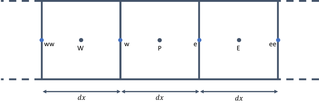
Once we approach the boundaries, we have to modify the discretised equation. To see this, consider the following sketch of the left end of the domain:
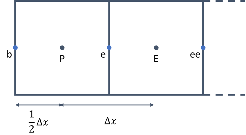
Here, we can see that we no longer have a value of the temperature at [katex]T^{n+1}_{i-1}[/katex] (or [katex]T^{n+1}_{W}[/katex]). Instead, we know the value at the boundary, which I have indicated here with the letter [katex]b[/katex]. If we indeed know the value at this point (in other words, we have a dirichlet-type boundary condition), then we can rewrite the discretised equation at point [katex]P[/katex], and we obtain the following equation:
T_{i+1}^{n+1}\left[\frac{\Gamma A}{\Delta x}\right]+T_i^{n+1}\left[\frac{-3\Gamma A}{\Delta x}\right]=T_b\left[\frac{-2\Gamma A}{\Delta x}\right]\tag{50}Or, using the location subscripts [katex]P[/katex], [katex]E[/katex], and [katex]W[/katex], as seen before, we can also write this as:
T_E^{n+1}\left[\frac{\Gamma A}{\Delta x}\right]+T_P^{n+1}\left[\frac{-3\Gamma A}{\Delta x}\right]=T_b\left[\frac{-2\Gamma A}{\Delta x}\right]
\tag{51}
This is for the left end of the domain; for the right side of the domain, we get the following discretised form:
T_i^{n+1}\left[\frac{-3\Gamma A}{\Delta x}\right]+T_{i-1}^{n+1}\left[\frac{\Gamma A}{\Delta x}\right]=T_{b}\left[\frac{-2\Gamma A}{\Delta x}\right]\tag{52}Again, we can write it with the location identifier [katex]P[/katex], [katex]E[/katex], and [katex]W[/katex] instead and arrive at:
T_P^{n+1}\left[\frac{-3\Gamma A}{\Delta x}\right]+T_W^{n+1}\left[\frac{\Gamma A}{\Delta x}\right]=T_{b}\left[\frac{-2\Gamma A}{\Delta x}\right]
\tag{53}
OK, so now that we have the discretised form, we need to implement that into our solver. Again, I have written about this source code as well, so you may want to look at my write-up for this 1D heat diffusion code for some background, which was developed in the context of creating our very own linear algebra library.
I have taken the same code and only replaced the parts where we are going to use Eigen now. I'll let you go through this code again first, and then we can discuss it below.
#include <iostream>
#include <cassert>

#include <Eigen/Eigen>

// solve the heat equation implicitly of the form dT/dt = gamma * d^2 T/ dx^2
// over a domain L using the conjugate gradient methdod
// initial condition: 0 everywhere
// boundary condition: T(0) = 0, T(L) = 1
int main() {
  // input variables
  const double gamma = 1.0;
  const unsigned numberOfCells = 100;
  const double domainLength = 1.0;
  const double boundaryValueLeft = 0.0;
  const double boundaryValueRight = 1.0;
  const double dx = domainLength / (numberOfCells);

  // vectors and matrices
  Eigen::SparseVector<double> coordinateX(numberOfCells);
  Eigen::SparseVector<double> temperature(numberOfCells);
  Eigen::SparseVector<double> boundaryConditions(numberOfCells);

  Eigen::SparseMatrix<double> coefficientMatrix(numberOfCells, numberOfCells);

  // initialise arrays and set-up 1D mesh
  for (unsigned i = 0; i < numberOfCells; ++i) {
    coordinateX.insert(i) = i * dx + dx / 2.0;
    temperature.insert(i) = 0.0;
    boundaryConditions.insert(i) = 0.0;
  }

  // calculate individual matrix coefficients
  const double aE = gamma / dx;
  const double aW = gamma / dx;
  const double aP = -2.0 * gamma / dx;

  // set individual matrix coefficients
  for (unsigned i = 1; i < numberOfCells - 1; ++i) {
    coefficientMatrix.insert(i, i) = aP;
    coefficientMatrix.insert(i, i + 1) = aE;
    coefficientMatrix.insert(i, i - 1) = aW;
  }

  coefficientMatrix.insert(0, 0) = -3.0 * gamma / dx;
  coefficientMatrix.insert(0, 1) = aE;
  coefficientMatrix.insert(numberOfCells - 1, numberOfCells - 2) = aW;
  coefficientMatrix.insert(numberOfCells - 1, numberOfCells - 1) = -3.0 * gamma / dx;

  // set boundary conditions
  boundaryConditions.coeffRef(0) = -2.0 * aW * boundaryValueLeft;
  boundaryConditions.coeffRef(numberOfCells - 1) = -2.0 * aE * boundaryValueRight;

  // solve the linear system using the conjugate gradient method
  Eigen::ConjugateGradient<Eigen::SparseMatrix<double>, Eigen::Lower | Eigen::Upper> CGSolver;
  CGSolver.compute(coefficientMatrix);
  CGSolver.setTolerance(1e-10);
  CGSolver.setMaxIterations(1000);
  temperature = CGSolver.solve(boundaryConditions);
  auto getIterations = CGSolver.iterations();

  // the obtain temperature profile is a linear one of the form T(x) = x. Thus, we can compare it directly against
  // the coordinate vector (which in this case acts as an analytic solution)
  auto difference = temperature - coordinateX;
  auto L2norm = difference.norm();

  // ensure that temperature has converged to at least single precision
  assert(L2norm < 1e-8);

  std::cout << "Simulation successful in " << getIterations << " iterations, final residual: " << L2norm << std::endl;
  return 0;
}This code produces the following output when I run it:
Simulation successful in 99 iterations, final residual: 3.87226e-15Since this is a simple model equation, and it is steady-state, and even 1D, we can let this converge down to machine precision (around [katex]10^{-16}[/katex]). Let's look at the code then together.
First, we define some common variables that relate to the simulation setup and mesh on lines 12-17. We include here the values of the temperature we want to reach on the left and right sides of the domain. As you can see, I use values of 0 and 1 here, indicating that we are dealing with non-dimensional temperature values, which we will use to our advantage at the end of the simulation.
On lines 20-24, I set up the required matrices and vectors, although strictly speaking, the coordinateX isn't really required here, I just create it here for completeness. We could have also made it a normal (dense) vector, e.g. using the Eigen::VectorXd type, there is no right or wrong here.
To make sense of the naming, if we consider the lienar system of equation [katex]\mathbf{Ax}=\mathbf{b}[/katex], then the coefficient matrix [katex]\mathbf{A}[/katex] is defined on line 24 and given the name coefficientMatrix, the solution vector [katex]\mathbf{x}[/katex] is our temperature sparse vector, as defined on line 21, and the right-hand side vector [katex]\mathbf{b}[/katex] is defined as boundaryConditions on line 22.
As we have seen from the discretised equation for the internal cells, i.e. Eq.(48), we do not have any contribution on the right-hand side, which is always zero here. However, once we approach the left and right side of the domain, we do end up generating some entries in our right-hand side vector, and for that reason, I have given the right-hand side vector [katex]\mathbf{b}[/katex] the explicit name boundaryConditions to make that clear and evident.
We then initialise our sparse vectors (and use the same loop to also compute the location of each cell's centroid) on lines 27-31. I use the insert(row) method here on each sparse vector, as this is the first time calling each vector, though I could have used coeffRef(row) here just as well.
I then go on to compute the coefficients for our internal domain, which I want to place in my coefficient matrix [katex]\mathbf{A}[/katex]. This is done on lines 34-36.
Notice that I have gotten rid of the area [katex]A[/katex] here (see Eq.(48)), as I assume that it is constant (and, in fact, given that this is a 1D discretisation, there is no concept of a face area, and I can make it as large or small as I want. A common choice is to set [katex]A=1[/katex], in which case it will vanish from the discretisation).
I then insert these [katex]a_P[/katex], [katex]a_E[/katex], and [katex]a_W[/katex] coefficients into my matrix on lines 39-43, but I skip the first and last row in my matrix, as these will need to be modified according to our boundary treatment.
I treat these boundaries next, by inserting values into our coefficient matrix into the first and last row. This is done on lines 45-48, and corresponds to the discretisation shown in Eq.(51) and Eq.(53). Since we also have a contribution on the right-hand side vector [katex]\mathbf{b}[/katex], we need to set that as well, which is done on lines 51-52.
With these steps done, we have assembled the coefficient matrix [katex]\mathbf{A}[/katex] and right-hand side vector [katex]\mathbf{b}[/katex], and all that is left to do is to throw some linear algebra solver at this system to compute an approximation to our solution vector [katex]\mathbf{x}[/katex], which in this case is our temperature vector.
All of this is done on lines 55-60. We first set up a linear system of equations solver on line 55. In particular, we use the Conjugate Gradient algorithm here, which is a pretty common choice for these types of elliptic equations.
If you look at the setup, you may wonder what the template parameters are. The first template parameter tells Eigen what type of matrix to expect. Since we defined our coefficient matrix on line 24 as Eigen::SparseMatrix, this is what the conjugate gradient solver should be expecting to receive, and so we state that here with the first template parameter.
The second is more interesting. Here, the second template parameter is set as Eigen::Lower | Eigen::Upper. First of all, the pipe symbol, i.e. |, indicates that we are dealing here with a concept known as a bitmask in C++. It is a concept you don't see frequently, and so if this is a new syntax to you, you may be excused.
A classic example of where you may want to use a bitmask is file writing. The C++ header fstream handles all file writing and reading to and from the disk. When we want to open a file, we may first create a file as std::ofstream file, which can be used to output a file. Then, we can call the open() method on this std::ofstream object as ```file.open("solution.dat").
This will open the file in writing mode, meaning that if the file already exists, it will overwrite the previous file. If, however, we wanted to tell the function to append to any existing files, we can indicate that with the second, optional parameter. For example, we can write file.open("solution.dat", std::ios::app), which will now append data instead.
But, you may want to further refine this open command and now require that all data be written in binary. If you still want to append data, which in turn should be written as binary data, then we would be in trouble if bitmasks didn't exist. But they do, and so what we can do is chain different configurations together as file.open("solution.dat", std::ios::app | std::ios::binary).
This will now append data and write it in binary representation. There are additional flags we could set here, and if you must know, you can look them up in the C++ reference here: std::ios_base::openmode.
Back to our example, on line 55, we specify the following options: Eigen::Lower | Eigen::Upper. We are telling Eigen that we have provided both the upper and lower triangle of the coefficient matrix. If we wanted, we could have simply provided only the upper triangle, meaning we would only have to set [katex]a_P[/katex] and [katex]a_E[/katex] coefficients. Since [katex]a_E=a_W[/katex] for internal nodes, Eigen could then infer the lower triangular part from the upper triangular part.
I have given both the upper and lower part, that is, we have written both [katex]a_E[/katex] and [katex]a_W[/katex] coefficients into our coefficient matrix [katex]\mathbf{A}[/katex], and I tell this to the conjugate gradient solver which now knows how to retrieve data from our sparse matrix (remember, a sparse matrix is just a storage container with some special behaviour to interpret stored data as a matrix).
In a real production run, you may want to only discretise either the upper or lower matrix and then save 33.3% on storage (since we are going to lose one of the three diagonals in our matrix). For educational purposes, I have left all of them in.
On line 55, we can also supply a third, optional parameter, which is the preconditioner. The preconditioner will modify our linear system of equations, i.e. [katex]\mathbf{Ax}=\mathbf{b}[/katex], in such a way that the solution for [katex]\mathbf{x}[/katex] is obtained with fewer iterations without affecting the solution accuracy.
Though this is where the limitations of Eigen start to show, as we don't really have any good preconditioners to use from. The three types that we have available are:
Eigen::IdentityPreconditionerEigen::DiagonalPreconditionerEigen::IncompleteLUT
The identity preconditioner isn't doing anything (great choice! Thanks Eigen!). It is like writing a calculator which offers the option to add a 0 to each calculation. The diagonal preconditioner is also better known as the Jacobi preconditioner, and the IncompleteLUT (lower-upper triangle) is probably the best (and only viable?!) choice available to us. You can try to add any of these as the third template parameter.
The incompleteLUT preconditioner drops the number of iterations to 0, meaning that the preconditioner essentially already finds the solution by itself, which can happen for these simple types of problems. But once you add complexities, and variable starts to depend on one another, preconditioners will not solve, but merely reduce the number of iterations required.
OK, we then go to line 56, where we use the compute(sparseMatrix) method on our conjugate gradient variable that we defined on line 55. The argument to this function is the coefficient matrix itself, and so, the name compute is perhaps not the best choice here. Something like setMatrix(matrix) may have been a better choice.
The reason Eigen uses the name compute(matrix) here is that, apart from setting the coefficient matrix, this method is doing a few more things, including the application of the preconditioner to our linear system of equations. Thus, there actually is some computations going on here, explaining the name, but if we don't have any preconditioner (as in our example), then this name is somewhat misleading.
On line 57, we set the tolerance for our conjugate gradient algorithm. We say that once the norm of the temperature is changing by less than [katex]10^{-10}[/katex] between two conjugate gradient iterations, we have reached a converged solution. On line 58, we supplement this setting with a max allowable number of iterations, and tell the solver that it should not be doing more than 1000 iterations, regardless of whether a solution could be obtained or not.
We should always set a max number of iterations to avoid a deadlock in which the solver isn't converging. This can easily happen with some more complicated linear solvers, especially when we start to use multigrids as preconditioners, but that is a whole different kind of problem; let's not get lost in that.
If you don't have anything else to go by, use 1000 iterations as a max number of iterations, and refine as necessary.
On line 59, we do some magic. We compute the solution of our linear system by calling the solve(b) method on our conjugate gradient variable. The parameter b is the right-hand side vector, i.e. the boundaryConditions vector in our code. We then inquire how many iterations it took to reach convergence, which we do on line 60.
Finally, I do exploit the fact here that the heat diffusion equation provides us with a linear temperature profile once converged, as long as there are no source terms in our domain. Our domain goes from [katex]x=0[/katex] to [katex]x=1[/katex], as we defined a domain length of 1 on line 14 and implied a start of the domain at [katex]x=0[/katex]. Furthermore, we set the boundary conditions for our temperature vector to [katex]T=0[/katex] on the left boundary (i.e. at [katex]x=0[/katex]) and [katex]T=1[/katex] on the right boundary (i.e. at [katex]x=1[/katex]).
Thus, once our temperature array has converged to a steady-state solution, we would expect that the temperature array and the x-coordinate have the same values at the cell centroids. I use this fact here on lines 64 and 65, where I first compute the difference between the two vectors (which should go to zero), and then compute the norm on this difference vector.
I check that we have converged to at least single precision on line 68 (i.e. [katex]10^{-8}[/katex]), which is reasonable, given that we set our convergence tolerance to [katex]10^{-10}[/katex], i.e. 2 orders of magnitude tighter.
This example does show how we can easily integrate Eigen into our implicit CFD solver environment. If I wanted to write a general-purpose CFD solver, I would probably not use Eigen due to its limitations in terms of what solvers are available. But, for something small where I don't want to be spending hours fine-tuning my linear solver setup, Eigen may just do the trick.
As a rule of thumb, I would say that if you are not looking at parallelising your code, Eigen is a solid choice. Once your problem size grows and you need your linear system of equations solver to grow with your problem sizes, you probably want to consider some alternatives (and we will look at libraries specifically designed for just solving linear systems of equations in this series, so don't worry, we will eventually get around to this topic as well).
At this point, we have seen all there is to Eigen, at least, all that is relevant to us. Eigen can do quite a bit, and there certainly are things we have not discussed that may be useful to your particular application, but for the most part, you will be using the things we have covered in this article.
However, before we close this section, I want to show you one more thing that I found quite cool when I first learned Eigen. In fact, the next section will show you an example of how to use Eigen in a completely different way to solve a common CFD problem.
Computing the flux Jacobian using automatic differentiation
Let me take you on a journey. The year is 2018, a Tuesday morning, just after Easter. I just passed my PhD viva, and, as is customary in the UK, I was presented with and feasting over my victory sandwiches, which I have since seen in every PhD viva where I have been either the internal or external examiner, both at my and other universities.
Stuffed and in a good mood, I found myself talking to my supervisors after the viva about potential post-doc positions. The interest was there, from both sides, but the money wasn't. There was an attempt to apply for funding, but that was unsuccessful. I was told they would try a few more options, and I should just stay put.
As I was just freshly engaged, with my better half working in Seoul about 10,000km away (for you Americans, that is a looooong distance), and me with no current source of income (nor fixed address), I thought I may just nest myself in her one-bedroom studio appartment for a few months, even though my tourist visa would only allow me to stay for 3 months. But that was a problem for future Tom, not present Tom.
So, put I stayed, for about 6 months, though in that time, no funding would materialise. To be able to stay for 6 months, I had to do some travelling, though, apparently, if you are on a tourist visa and you are entering a country without any return flight, this is suspicious (who would have thought), and so the check-in assistant at Osaka airport made me sign a declaration stating that I am aware that I have to leave the country after my visa expires or legal actions may be taken against me.
I was disappointed, after all, Germany and Japan used to work very well together, and I was hoping for better treatment, but I suppose we have lost that special connection since 1945 ... Now I was that German refugee trying to illegally enter an asian country, I think that must have been a first.
Without any funding on the horizon, and being tired and frustrated of waiting (as well as a domestic dispute that, apparently, I cannot just stay home and program games (I was really deep into game programming at that time), while my wife (yes, we got married in the meantime) was working).
So, I had to look for positions and applied for one at the German Aerospace Center (DLR), which happily welcomed me back home from my extended period abroad. The year was still 2018, 2 years after the Brexit referendum, but before any Brexit agreement was signed, and so my interview consisted mostly of geopolitical questions, infused with a few questions about multigrids, parallelisation, and C++ programming.
The interview took place on a Friday afternoon. I was travelling back from South Korea the day prior and was still a bit jetlagged, but apparently they enjoyed the interview so much that they spent 4 hours talking to me, instead of the usual 1 hour. I got the job the following week, accepted, moved to Braunschweig and had a fantastic 14 months there.
I say fantastic, because on the job is where I was first introduced to Eigen. Love at first sight. Initially, I didn't notice that I fell in love with the library, but at some point, I realised that I cannot live without the library in any of my other programming projects anymore.
I used Eigen for everyday, 3D linear algebra stuff, similar to the examples we have looked at in this article. But then, one day, I came across the file in which we were computing the flux Jacobian, and I didn't quite comprehend what we were doing here. To understand that, let's look at the flux Jacobian for a second.
Let's assume we are using the Euler equation. For simplicity, we are going to use the 1D Euler equation, which we can write as:
\frac{\partial \mathbf{U}}{\partial t}+\frac{\partial \mathbf{F}}{\partial \mathbf{x}}=0
\tag{54}
We have the vector of conserved variables [katex]\mathbf{U}[/katex] as:
\mathbf{U}=
\begin{bmatrix}
\rho \\[0.5em]
\rho u\\[0.5em]
\rho E
\end{bmatrix}
\tag{55}
The fluxes [katex]\mathbf{F}[/katex] are given as:
\mathbf{F}=
\begin{bmatrix}
\rho u \\[0.5em]
\rho u^2 + p \\[0.5em]
u(\rho E + p)
\end{bmatrix}
\tag{56}
A common task we need to do is to form the Flux Jacobian [katex]\partial\mathbf{F}/\partial\mathbf{U}[/katex], that is, how do the fluxes change with respect to the conserved variable vector?
For example, for compressible flows, we like to use Riemann solvers, as they are the gold standard for treating discontinuities (e.g. shock waves), across which flow properties change instantaneously on the macroscale (on the microscale, over a few atomic diameters, changes are smooth again).
And, if you are an OpenFOAM developer, you must be suffering from R-SAD (Riemann Solver Avoidant Disorder). Seriously, how do we still not have Riemann solvers in OpenFOAM in the 21st century? rhoCentralFoam shows that this can be done, and this shouldn't be a difficult feature to implement.
Wait, what? OpenFOAM was developed at Imperial College? Oh boy, that certainly explains things ... If you haven't read my Imperial College review, now may be a good time to catch up (or not, it has no impact on the current discussion whatsoever)
Let's look at the Roe Riemann solver, a quite popular Riemann solver which was developed by Philip Roe in 1981. Roe would move to Cranfield University in 1984 and stay until 1990, and be, to the best of my knowledge, the course director for the MSc in CFD, a course created by the godfather of Riemann solvers, Eleuterio Toro.
Some of you may know that I am the course director for the same course (and if you read this in the future, I may no longer be the course director, it seems we have a shelf lives of only a few years, after which, Cranfield finds some other, new, exciting things for us to work on (for example, the QS working group (that will only make sense if you read the Imperial College rant))).
Suffice it to say, knowing the history of the course, I don't feel that I am a match for my former colleagues. I mean, they have essentially paved the way for compressible flow CFD; meanwhile, I have a CFD blog. And, as Milo Edwards would say, 1 blog is one too many (though he uses that in the context of podcasts, let's not split hairs).
In any case, Riemann solvers, Roe, let's get back on track. One of the key principles of Roe's Riemann solver is a local linearisation step. Let's look at the Euler equation again, i.e. Eq.(54). Here, the fluxes [katex]\mathbf{F}[/katex], as shown in Eq.(56), have a non-linear dependence on the velocity [katex]u[/katex] (the second entry has the term [katex]\rho u^2[/katex], i.e. we multiply [katex]u[/katex] with itself, making it non-linear).
Our goal is to linearise these fluxes. Why, you may ask? Well, we are missing a bit of knowledge here about Riemann problems in general, but let's just say that if we wanted to solve the non-linear Riemann problem exactly, we would have to do so using an iterative approach, which is expensive.
If we can, however, linearise our system of equations, we can remove the need for iterating, which makes our system we solve very cheap. And if there is one thing we love in CFD, it is reducing computational cost through any means possible.
To further understand what Roe is doing with his Riemann solver, let's review the chain rule again, and let me give you an example that may help you understand why the chain rule is so important.
Let's say I want to model how fuel flow [katex]f[/katex] to an aircraft engine changes with altitude [katex]h[/katex]. The mathematical question I am trying to answer here is, what is [katex]\mathrm{d}f/\mathrm{d}h[/katex]? This may be difficult to measure and calculate directly. However, there are other quantities, like speed, that are affected by the aircraft's altitude and will have an effect on the fuel flow.
For example, if we reduce the fuel flow to the engine, our velocity will drop. If we increase the fuel flow to our engine, then the speed will increase. I think we can all agree on that. In other words, there is a very clear connection between the velocity [katex]u[/katex] and the fuel flow [katex]f[/katex], and so evaluating the derivative [katex]\mathrm{d}f/\mathrm{d}u[/katex] is not difficult.
And, if you are like me, as a student, I had a phobia of differentials, and so to make this point very clear, let's say we measure that the fuel flow is 850 kg/hour at a speed of 500 km/h. If we decrease the velocity to 400 km/h, we measure a fuel flow of 680 kg/hour. With these numbers, we can numerically compute our derivative as:
\frac{\mathrm{d}f}{\mathrm{d}u} = \frac{f_1 - f_0}{u_1 - u_0} = \frac{850 - 680}{500 - 400} = \frac{170}{100} = 1.7\tag{57}Remember, all that the [katex]\mathrm{d}[/katex] symbol tells us is that we are looking at differences (between two points/states/etc.). This is what I have used in the equation above, e.g. replacing [katex]\mathrm{d}f[/katex] by [katex]f_1-f_0[/katex]. Mathematically speaking, the derivative becomes exact as our denominator difference (here the velocity difference) goes to zero, but if we assume a linear relationship, we do get a good estimate, even if [katex]\mathrm{d}u[/katex] is further away from zero, as is the case here.
In any case, we have computed [katex]\mathrm{d}f/\mathrm{d}u[/katex], what have we gained? Not much, yet. But we can now link the velocity to the altitude. We can ask, how does velocity change with altitude, if otherwise all other parameters are the same? Well, from aerodynamics 101, we know that lift is computed as:
L=\frac{1}{2}C_L\rho u^2 S\tag{58}Lift is a function of both u (our velocity) and the density ([katex]\rho[/katex]). The density will change with different altitudes, which we can compute from the international standard atmosphere (ISA). As we fly higher, the air will decrease in density, and so with all other quantities remaining the same, the velocity will increase. This makes sense; fewer air molecules mean lower density, but also less drag, and so a greater velocity.
Let's use some example calculation again and say that at a height of 25,000 feet, we have a density of [katex]0.55\,kg/m^3[/katex]. At a height of 30,000 feet, we may have a density of [katex]0.45\,kg/m^3[/katex].
Since we assume all other quantities in the lift equation to remain constant, we can simply form the ratio of the lift equation at these two different altitudes and find an equation for the velocity as a dependence on the density. This is shown in the following derivation:
\frac{L_{25,000\,ft}}{L_{30,000\,ft}} = \frac{\frac{1}{2}C_L\rho_{25,000\,ft}u_{25,000\,ft}^2S}{\frac{1}{2}C_L\rho_{30,000\,ft}u_{30,000\,ft}^2S}\\[1em]
1 = \frac{\rho_{25,000\,ft}}{\rho_{30,000\,ft}}\frac{u_{25,000\,ft}^2}{u_{30,000\,ft}^2}\\[1em]
1=\frac{0.55}{0.45}\frac{u_{25,000\,ft}^2}{u_{30,000\,ft}^2}\\[1em]
\frac{0.45}{0.55}=\frac{u_{25,000\,ft}^2}{u_{30,000\,ft}^2}\\[1em]
u_{25,000\,ft}^2=\frac{0.45}{0.55}u_{30,000\,ft}^2\\[1em]
u_{25,000\,ft} = \sqrt{\frac{0.45}{0.55}u_{30,000\,ft}^2}\tag{59}
So, if we know the velocity at 30,000 feet to be, say 200 m/s, then we can compute the velocity at 25,000 feet as:
u_{25,000\,ft} = \sqrt{\frac{0.45}{0.55}200^2} \approx 181\,m/s\tag{60}With these numbers, we can now find, again, a simple way to establish how the velocity changes with altitude. We can express that as a derivative again as [katex]\mathrm{d}u/\mathrm{d}h[/katex], and we can compute this with the numbers we have produced as:
\frac{\mathrm{d}u}{\mathrm{d}h}=\frac{u_1-u_0}{h_1-h_0}=\frac{200-181}{9144 - 7620}=\frac{19}{1524} \approx 0.0125\tag{61}I have converted these feet into meters ([katex]25,000\, ft = 7620\, m[/katex] and [katex]30,000\, ft = 9144\, m[/katex]), to be consistent with our units (as velocity is given in meter per second, not feet per second).
So, let's step back for just one second and see what we have achieved. We wanted to know how fuel flow changes with a change in altitude, that is, [katex]\mathrm{d}f/\mathrm{d}h[/katex]. However, we found this difficult to obtain, and so, instead, we found other derivatives that relate to both [katex]f[/katex] and [katex]h[/katex], which were easy to form.
Using the chain rule, we can now bring all of this together. The chain rule just states that we can chain different derivatives together, as long as these are consistent. So, in our case, we can write our derivative [katex]\mathrm{d}f/\mathrm{d}h[/katex] as a function of the velocity as:
\frac{\mathrm{d}f}{\mathrm{d}h}=\frac{\mathrm{d}f}{\mathrm{d}u}\frac{\mathrm{d}u}{\mathrm{d}h}\tag{62}We have already computed these derivatives on the right-hand side, and so, we can now compute how the fuel flow changes as a result of a change in altitude as:
\frac{\mathrm{d}f}{\mathrm{d}h}=\frac{\mathrm{d}f}{\mathrm{d}u}\frac{\mathrm{d}u}{\mathrm{d}h}=1.7\cdot 0.0125=0.02125\tag{63}I said that we have to apply the chain rule consistently. What I mean by that is that the denominator to the left must appear in the numerator to the right in the product of our chain rule. The first term has [katex]u[/katex] in its denominator, and so it must appear in the numerator to its right (i.e. the second term), which it does. If we wanted, we could extend this chain rule arbitrarily.
For example, we saw that the velocity really changes with density, and so we could evaluate the derivative [katex]\mathrm{d}u/\mathrm{d}\rho[/katex], and we also said that the density changes with height, that is, [katex]\mathrm{d}\rho/\mathrm{d}h[/katex]. So, we could have generalised our chain rule to:
\frac{\mathrm{d}f}{\mathrm{d}h}=\frac{\mathrm{d}f}{\mathrm{d}u}\frac{\mathrm{d}u}{\mathrm{d}\rho}\frac{\mathrm{d}\rho}{\mathrm{d}h}\tag{64}The key takeaway here is that the chain rule allows us to replace derivatives that are otherwise difficult to obtain by a product of derivatives that are, all on their own, easy to compute.
To put this onto more firm grounding, consider the following function:
f(x)=\sqrt{1-x^2}\\[1em]
f(x)=(1-x^2)^{1/2}\tag{65}
We could now look back at our high-school definitions of how to find the derivative of this function, where we first differentiate the inner term and then the outer. We would obtain the following derivative:
f'(x)=\frac{1}{2}(1-x^2)^{-1/2}2x\\[1em]
f'(x)=\frac{x}{\sqrt{1-x^2}}
\tag{66}
However, we could also use the chain rule here to make our lives easier. To do that, we define a new function [katex]u[/katex], which we substitute into our original equation. This gives us:
u = 1-x^2\\[1em]
f(x) = \sqrt{u}\tag{67}
So, we want to find how our function [katex]f(x)[/katex] changes with respect to [katex]x[/katex], that is, we want to find [katex]\mathrm{d}f/\mathrm{d}x[/katex]. As we saw, we can directly evaluate this expression, or, we can use the chain rule again. To do that, we first need to know how our function [katex]f(x)[/katex] changes with [katex]u[/katex], and then how [katex]u[/katex] changes with [katex]x[/katex]. We can write this as:
\frac{\mathrm{d}f}{\mathrm{d}x}=\frac{\mathrm{d}f}{\mathrm{d}u}\frac{\mathrm{d}u}{\mathrm{d}x}\tag{68}Let's compute the first derivative. We have:
\frac{\mathrm{d}f}{\mathrm{d}u}=\frac{\mathrm{d}}{\mathrm{d}u}\sqrt{u}=\frac{\mathrm{d}}{\mathrm{d}u}u^{1/2}=\frac{1}{2}u^{-1/2}=\frac{1}{2\sqrt{u}}\tag{69}Next, let's see how [katex]u[/katex] changes with [katex]x[/katex]. This gives us:
\frac{\mathrm{d}u}{\mathrm{d}x}=\frac{\mathrm{d}}{\mathrm{d}x}(1-x^2)=2x\tag{70}As per the chain rule, we can now put both of these derivatives together, and we obtain:
\frac{\mathrm{d}f}{\mathrm{d}x}=\frac{\mathrm{d}f}{\mathrm{d}u}\frac{\mathrm{d}u}{\mathrm{d}x}=\frac{1}{2\sqrt{u}}2x=\frac{x}{\sqrt{1-x^2}}\tag{71}This is exactly what the derivative should be, as we already saw in Eq.(66). So, to recap, again, the chain rule allows us to decompose a derivative into easier-to-model parts.
How does that relate to the Roe Riemann solver? Let's look at the Euler equation again:
\frac{\partial \mathbf{U}}{\partial t}+\frac{\partial \mathbf{F}}{\partial \mathbf{x}}=0\tag{72}As we discussed, we have a non-linear term in our fluxes [katex]\mathbf{F}[/katex], that is, we have a term where we multiply the velocity by itself ([katex]\rho u^2[/katex]). Roe is now linearising the fluxes using the following chain rule:
\frac{\partial \mathbf{U}}{\partial t}+\frac{\partial \mathbf{F}}{\partial \mathbf{U}}\frac{\partial \mathbf{U}}{\partial \mathbf{x}}=0\\[1em]
\frac{\partial \mathbf{U}}{\partial t}+\mathbf{A}_{Roe}(\mathbf{U})\frac{\partial \mathbf{U}}{\partial \mathbf{x}}=0\tag{73}
Here, [katex]\mathbf{A}_{Roe}(\mathbf{U})=\partial \mathbf{F}/\partial \mathbf{U}[/katex] is the so-called flux Jacobian. This equation is still exact. That is, if we had an analytic solution for the Navier-Stokes equation, then both this equation and the original equation would give us exactly the same answer, and this equation is still non-linear. So we haven't gained anything yet.
This is where Roe introduced the approximation by saying that the flux Jacobian [katex]\mathbf{A}_{Roe}(\mathbf{U})[/katex] can be treated as a constant coefficient matrix, if we do that, then we can essentially treat [katex]\mathbf{A}_{Roe}(\mathbf{U})[/katex] as some form of coefficient, multiplying the conserved variable derivative vector, i.e. [katex]\partial \mathbf{U}/\partial \mathbf{x}[/katex]. Since [katex]\mathbf{U}[/katex] is linear, making [katex]\mathbf{A}_{Roe}(\mathbf{U})[/katex] a constant coefficient matrix will make the modified equation a linear equation.
To indicate that [katex]\mathbf{A}_{Roe}(\mathbf{U})[/katex] is constant, it is typically replaced by the notation [katex]\mathbf{A}_{Roe}(\mathbf{\tilde{U}})[/katex]. So, now that we have a linear equation, we can avoid expensive iterations to solve our Riemann problem, at the cost of having introduced a linearisation to a non-linear problem. As long as our grid resolution is good enough to resolve flow structures, however, this linearisation step does not pose any limitations in practice. In fact, the Roe Riemann solver is one of the most widely used ones, and probably for a good reason.
So, let's then turn our attention to the flux Jacobian [katex]\partial \mathbf{F}/\partial \mathbf{U}[/katex]. This can be computed as:
\frac{\partial \mathbf{F}}{\partial \mathbf{U}}=
\begin{bmatrix}
0 & 1 & 0 \\[1em]
\frac{\gamma-3}{2} u^2 & (3-\gamma) u & \gamma - 1 \\[1em]
u \left(\frac{\gamma-1}{2} u^2 - H\right) & H - (\gamma-1) u^2 & \gamma u
\end{bmatrix}, \quad
H = \frac{E + p}{\rho}\tag{74}
The pressure can be computed as:
p = (\gamma - 1) \left( E - \frac{1}{2} \frac{(\rho u)^2}{\rho} \right) = (\gamma - 1) \left( E - \frac{1}{2} \rho u^2 \right)\tag{75}Here, [katex]\gamma[/katex] is the ratio of specific heats, which for air is [katex]\gamma=c_p/c_v=1.4[/katex]. We can now form this flux Jacobian directly, but this is only for a 1D flow. What happens if we have a 2D or 3D flow? Then we have to re-derive this flux Jacobian. What if we want to solve the compressible Navier-Stokes equations, not just the inviscid Euler equations? We have to re-derive the flux Jacobian. And what happens if we start to have source terms to include additional physics? You guessed it, we have to re-derive the flux Jacobian.
Now, don't get me wrong, this can be done, but if I told you you can avoid all of that and simply go about computing your fluxes and then call a magic function on your fluxes [katex]\mathbf{F}[/katex] that would give you the derivatives, would you not rather do that? Well, my friend, Eigen lets you do exactly that!
To do this, Eigen uses a concept known as automatic differentiation. It hasn't really gained a lot of traction in the field of CFD (I am sure there still are many CFD practitioners who have never come across the term automatic differentiation), but, if we look a bit at other fields, like machine learning, for example, automatic differentiation is such an important concept that we cannot do anything without it. Automatic differentiation is to machine learning what solving a linear system of equations is to CFD.
To understand how we can use automatic differentiation in Eigen, we first should review what it does under the hood, so we have a shared understanding of this magical tool.
Let's consider an arbitrary function [katex]f(x)[/katex]. As a CFD engineer, or any engineer for that matter, we are commonly tasked with finding the derivatives of a specific function, i.e. [katex]\mathrm{d}f(x)/\mathrm{d}x[/katex]. There are two methods we can use that we should all already be familiar with:
- If [katex]f(x)[/katex] has a symbolic representation, then we can obtain a symbolic formula for the derivative. For example, the symbolic function [katex]f(x)=x^2[/katex] has the derivative of [katex]f'(x)=2x[/katex]. We can now compute the derivative [katex]\mathrm{d}f(x)/\mathrm{d}x[/katex] at any point in [katex]x[/katex] exactly, using our analytic/symbolic formula.
- If [katex]f(x)[/katex] does not have a symbolic function, but we have data points, e.g. from measurements (similar to our fuel flow example, where we had fuel flow and velocity measurements), we can compute the derivative numerically, typically through the use of the Taylor series. This is the basis for the finite difference method.
Automatic differentiation uses a different approach. It states that any computation can be broken down into a set of smaller operations. Once broken down sufficiently, all that we are left with are basic operations for which we know how to form the derivative. To find the overall derivative of an entire expression, we use the chain rule to put all derivatives together.
Let's look at a concrete example. Let's go back to our function we looked at previously:
f(x)=\sqrt{1-x^2}\\[1em]
f(x)=(1-x^2)^{1/2}\tag{76}
We know that the derivative can be computed as:
f'(x)=\frac{1}{2}(1-x^2)^{-1/2}2x\tag{77}Ok, but let's now assume that all we have is the function [katex]f(x)[/katex], and we want to find the derivative at a specific location of [katex]x[/katex] (that could be, for example, at the cell centroid, or at faces, etc.).
For the sake of argument, let's say we want to evaluate the function at [katex]x=0.25[/katex]. We can compute the derivative as:
f'(x=0.25)=\frac{1}{2}(1-x^2)^{-1/2}2x=\frac{1}{2}(1-0.25^2)^{-1/2}2\cdot 0.25 \approx 0.25819889\tag{78}We will use that to compare our results from the automatic differentiation later, but I should stress here again that we don't generally have this analytic derivative available.
So, we need to break down this function into elementary operations, for which we do know how to find the derivative. The breakdown of:
f(x)=(1-x^2)^{1/2}\tag{79}can be written in the following way:
- [katex]x=0.25[/katex]
- [katex]u(x)=x^2[/katex]
- [katex]v(u)=1-u[/katex]
- [katex]f(v)=v^{1/2}[/katex]
If we can find the derivatives of these individual functions, then we can form the derivative [katex]\mathrm{d}f/\mathrm{d}x[/katex] as a combination of the derivatives as a chain rule. This can be written as:
\frac{\mathrm{d}f}{\mathrm{d}x}=\frac{\mathrm{d}f}{\mathrm{d}v}\frac{\mathrm{d}v}{\mathrm{d}u}\frac{\mathrm{d}u}{\mathrm{d}x}\frac{\mathrm{d}x}{\mathrm{d}x}\tag{80}What we then do, in automatic differentiation, is to keep track of both the function value for each operation, as well as the derivative for that elementary operation. Later, we will simply multiply all derivatives together and get our final derivative.
So, let's compute the derivative with automatic differentiation. I'll start at the back. We have already set [katex]x=0.25[/katex]. The derivative [katex]x[/katex] with respect to [katex]x[/katex] is 1, and we write this as [katex]x'=1[/katex].
For the second term, it gets a bit more interesting. Here, we want to differentiate [katex]u[/katex] with respect to [katex]x[/katex], that is, we want to compute [katex]\mathrm{u}/\mathrm{d}x[/katex] for [katex]u(x)=x^2[/katex]. We can write this function as well as [katex]u(x)=x\cdot x[/katex]. This is a simple multiplication, and, for multiplications, we can use the product rule to find the derivative. It is given for two arbitrary variables [katex]a[/katex] and [katex]b[/katex] as:
(ab)'=a'b + ab'\tag{81}In our example, we have [katex]a=b=x[/katex], and so, we could also write this as:
(xx)'=x'x + xx'\tag{82}We already know what [katex]x[/katex] is, that is, the value we have specified at the beginning, where we want to evaluate the derivative at, i.e. [katex]x=0.25[/katex]. We also know its derivative, which we computed in the previous step, i.e. [katex]x'=1[/katex]. So, we can insert these values into the product rule and get:
(xx)'=x'x + xx'=1\cdot 0.25 + 0.25 \cdot 1 = 0.5\tag{83}Well, that makes sense, doesn't it? If we look at the underlying elementary operation, i.e. [katex]x^2[/katex], we could find the derivative ourselves as [katex]2x[/katex]. If we insert the value of [katex]x=0.25[/katex], then we get a value of [katex]0.5[/katex], which is exactly the same as we have computed with our automatic differentiation step.
Now we need to keep track of this derivative. We store this derivative as [katex]u'=0.5[/katex], and we also evaluate the function itself now. We have [katex]u(x)=x^2=0.25^2=0.0625[/katex]. To recap, we have thus far found the following function values:
x=0.25\qquad u=0.0625\tag{84}They have the corresponding derivatives of:
x'=1\qquad u'=0.5\tag{85}And now, we just go through the rest of our expression and rinse and repeat. Our next expression is [katex]v(u)=1-u[/katex]. We know the value for [katex]u[/katex], which we just computed as [katex]u=0.0625[/katex]. Thus, we can compute the value of [katex]v[/katex] as [katex]v(u=0.0625)=1-0.0625=0.9375[/katex].
For the derivative, we need to differentiate the expression [katex]1-u[/katex] with respect to x. If we differentiate 1 with respect to [katex]x[/katex], well, we are differentiating a constant, which doesn't change, so the result is 0. In other words, [katex]\mathrm{d}1/\mathrm{d}x=0[/katex]. So, we only need to focus on the second part, that is, [katex]-u[/katex].
Since the dependent variable of [katex]v(u)[/katex] is [katex]u[/katex], we need to differentiate it with respect to [katex]u[/katex]. So, the question is, what is [katex]-u[/katex] differentiated with respect to [katex]u[/katex]? Well, [katex]\mathrm{d}-u/\mathrm{d}u=-1[/katex]. So, in this step, we have found that [katex]v=0.9375[/katex] and [katex]v'=-1[/katex].
One more to go. The final expression is [katex]f(v)=v^{1/2}[/katex]. Let's find [katex]f(v=0.9375)[/katex] first. Inserting [katex]v[/katex], we get: [katex]f(v)=0.9375^{1/2}\approx 0.96824584[/katex]. What about the derivative?
Well, we can find that using standard rules for differentiation of an exponent:
f'(v)=\frac{1}{2}v^{-1/2}=\frac{1}{2\sqrt{v}}\tag{86}Inserting the value for [katex]v=0.96824584[/katex], we obtain the following derivative for [katex]f'(v)[/katex]:
f'(v=0.96824584)=\frac{1}{2\sqrt{0.96824584}}\approx 0.50813275\tag{87}Ok, let's recap what we have obtained. We got the following derivatives:
x'=1\qquad u'=0.5\qquad v'=-1\qquad f'= 0.50813275\tag{88}We could also write these derivatives with respect to the variables that we have differentiated them by:
\frac{\mathrm{d}x}{\mathrm{d}x}=1\qquad \frac{\mathrm{d}u}{\mathrm{d}x}=0.5\qquad \frac{\mathrm{d}v}{\mathrm{d}u}=-1\qquad \frac{\mathrm{d}f}{\mathrm{d}v}=0.50813275\tag{89}Remember our chain rule? We had:
\frac{\mathrm{d}f}{\mathrm{d}x}=\frac{\mathrm{d}f}{\mathrm{d}v}\frac{\mathrm{d}v}{\mathrm{d}u}\frac{\mathrm{d}u}{\mathrm{d}x}\frac{\mathrm{d}x}{\mathrm{d}x}\tag{90}So, let's insert all of these simpler derivatives and chain them together to get the final derivative we are seeking. We get:
\frac{\mathrm{d}f}{\mathrm{d}x}=1\cdot 0.5\cdot -1\cdot 0.50813275 = -0.254066375\tag{91}Let's compare that against the derivative, which we have computed using the analytic function. There, we obtained f'(x)=0.25819889. That's pretty close, and the main reason we are not seeing a better agreement is that we have truncated the numbers somewhat. But, you see, whenever we have a computation to perform, we can keep track of the computation itself and then compute the derivative for each elementary operation.
So, let's implement this simple function into Eigen using automatic differentiation, to ease us in. We will get to the Jacobian example afterwards, but for now, let's implement [katex]f(x)=\sqrt{1-x^2}[/katex] into Eigen and see how well it can perform the derivative. The code is shown below, and we will discuss it afterwards together in detail.
#include <iostream>
#include <Eigen/Dense>
#include <unsupported/Eigen/AutoDiff>

// AutoDiff scalar type
using ADScalar = typename Eigen::AutoDiffScalar<Eigen::VectorXd>;

int main()
{
    ADScalar x;
    x.value() = 0.25;
    x.derivatives() = Eigen::VectorXd::Unit(1, 0);

    ADScalar f = Eigen::sqrt(1.0 - Eigen::pow(x, 2));

    std::cout << "f(x):  " << f.value() << std::endl;
    std::cout << "df/dx: " << f.derivatives()(0) << std::endl;

    return 0;
}This code produces the following output:
f(x):  0.968246
df/dx: -0.258199Let's compare that with our analytic results first, which we have calculated by hand. The function value is [katex]f(x=0.25) = 0.968246[/katex], no surprise here. And, for the derivative? We get [katex]f'(x)=-0.258199[/katex]; that is exactly the same (down to the last digit) as our analytic derivative, where we obtained [katex]f'(x)=-0.25819889[/katex]. Accounting for round-off differences, these numbers are identical, and that is the power of automatic differentiation!
But let's now turn our attention to the code itself to understand what is happening here. We import the necessary includes first. As I have no use for sparse matrices or vectors here, i.e. in this example I'm only using dense vectors, I included the Eigen/Dense header on line 2, but I could have also included the usual Eigen/Eigen header.
On line 3, I am exposing Eigen's automatic differentiation. What you'll see is that it lives in the unsupported/Eigen/AutoDiff header. The name is somewhat misleading. I did find bugs in their automatic differentiation module, and they fixed it pretty quickly. So, perhaps, the header maybeSupported/Eigen/AutoDiff would have been more accurate, but what do I know.
In any case, they do have a few extra bits and bobs implemented for which they have, apparently, no plans to bring this over to the main code base, and if you want to browse through the different things they have implemented, you can browse through the source code yourself.
You'll find additional iterative solvers (like GMRES, amazing!), wrappers for OpenGL (perhaps not as relevant here, though we will touch upon that later in this series, and we will learn how painful OpenGL is (if I hate myself enough to come up with a CFD example (everytime I touch OpenGL I losse about a year of life expectancy))), Splines, and Polynomials, to name but a few.
Usually, I am quick to point out how great Eigen's documentation is, but in the case of the unsupported headers, the unsupported status seems to have been applied to some of the documentation as well. For example, looking at the numericalDiff header file, it reads:
"It is very easy for you to write a functor using such [proprietary and free] software, and the purpose is quite orthogonal to what we want to achieve with Eigen."
Say what? Did I mention the French are behind the development of Eigen? That, perhaps, explains things. Let's not speak of it again ...
OK, retour à notre code, we define a scalar on line 6, which is essentially just a double. But, it is a very special kind of scalar; this is a scalar that can hold both a number like any other scalar and a derivative. Looking at the type of this ADScalar, as I have named it, it is of type Eigen::AutoDiffScalar, which, in turn, takes one template argument, which is Eigen::VectorXd.
We have looked at Eigen::VectorXd before, and we know that Xd in VectorXd stands for a dynamically-sized vector (that is, the X), where the entries in the vector are stored as double. That is all good, but why is our ADScalar a vector?
Well, the ADScalar has to not only hold our value, but also the derivatives. And, in theory, we can have an arbitrary number of derivatives. For example, in our example, we have just one independent variable, and we take our derivatives with respect to that. This is also indicated by our function, i.e. [katex]f(x)[/katex], where [katex]x[/katex] is the only independent variable.
But if we are dealing with the Navier-Stokes equation, then we have multiple independent variables. For example, the velocity in the x-direction can be written as [katex]u = f(t,x,y,z)[/katex], that is, the velocity component [katex]u[/katex] has 4 independent variables, and so it can have 4 different derivatives, that is, [katex]\partial u/\partial t[/katex], [katex]\partial u/\partial x[/katex], [katex]\partial u/\partial y[/katex], and [katex]\partial u/\partial z[/katex].
For this reason, our ADScalar must store a vector, and we typically use here the dynamically-sized vector Eigen::VectorXd so that we don't have to worry about the exact number of entries in our vector, which will later hold the values of our derivatives. The size of the vector will be the same as the number of independent variables.
But, just to be clear, if you wanted to, you could replace Eigen::VectorXd here for Eigen::Matrix, as we only have a single derivative. If we had 2, 3, or more, then we could also write Eigen::Matrix, Eigen::Matrix, or Eigen::Matrix, where the last example is the same as just writing Eigen::VectorXd.
OK, so now that we have created this cool new type, let's apply that to a simple calculation. On line 10, I define a scalar x. Remember, x is our independent variable, and so this has to be treated as an ADScalar, and we will see in a second why. We might be tempted to just use a double instead, after all, all that we are assigning to the value of x is the location at which we want to evaluate the derivative, right?
Yes, this is correct, but we declare it as an ADScalar and we give it some special properties so that Eigen knows that this is our independent variable. It might not make sense to us, but Eigen somehow needs to be told what is and what isn't an independent variable, and this is how they have decided to handle things. Sacrebleu ...
OK, so on line 11, we call the value() method on our x scalar, which allows us to set the value for [katex]x[/katex]. In our case, [katex]x=0.25[/katex]. But then, we proceed with our Eigen magic and call the derivatives() method on x as well. If you recall, when we computed the derivative manually through the chain rule, we had one term that states [katex]\mathrm{d}x/\mathrm{d}x=1[/katex]. In other words, [katex]x[/katex] differentiated with respect to itself is 1.
Now, we call the derivatives() function on our scalar x (e.g. our independent variable), and we set that equal to Eigen::VectorXd::Unit(1, 0). What is going on here? The call to Unit(1, 0) tells Eigen that we want to create a unit vector, which has a length/size of 1 (first argument, that is, how many independent variables we have), and we tell it the index which should be set to 1 (which, in this case, is index 0).
This is somewhat confusing, but let me expand on this and give you an additional example. Let's say we now have two independent variables, so that our function becomes [katex]f(x,y)[/katex] and we want to compute derivatives with respect to [katex]x[/katex] and [katex]y[/katex]. In this case, our ADScalar type remains the same. Remember, we gave the template argument of Eigen::VectorXd, which will dynamically grow with the number of derivatives to evaluate.
So, we would then create two ADScalar for both x and y, and then, proceed with the following lines:
x.derivatives() = Eigen::VectorXd::Unit(2, 0);y.derivatives() = Eigen::VectorXd::Unit(2, 1);
Here, we are now specifying to the Unit() method that we want to create a unit vector of size/length 2, and in the case of the x scalar, we set the first index to 1 (that is the second argument, i.e. index 0 is set to 1), while for y, we have the same length but we set the second index to 1 (that, is the second argument, which is set to 1).
We can write this in equation form to see what [katex]x[/katex] and [katex]y[/katex] represent here mathematically. We have:
x = \left[\frac{\partial x}{\partial x},\frac{\partial x}{\partial y}\right] = [1, 0] \\[1em]
y = \left[\frac{\partial y}{\partial x},\frac{\partial y}{\partial y}\right] = [0, 1] \tag{92}
In a nutshell, all that we are specifying here is what the derivatives of our independent variables are with respect to each other. It is always the same pattern, i.e. we always use the Unit(size, indexAtWhichVectorIsOne) method to let Eigen now how the independent variables differentiate with respect to each other, and so later, when Eigen is doing the automatic differentiation for us, and comes across [katex]\mathrm{d}x/\mathrm{d}x[/katex], or [katex]\mathrm{d}y/\mathrm{d}y[/katex] in the chain rule, it knows how to treat this specific value.
Hopefully, this is clear; this is probably the most difficult part to understand about automatic differentiation in Eigen, but other packages will have to implement this somehow as well.
A quick survey shows that AutoDiff, for example, handles that a bit nicer. In their case, we would specify that x is an independent variable by writing double X = derivative(f, wrt(x), at(x,y,z));. I think we can all agree this is a bit cleaner and more expressive than setting the unit vector.
Or, take FADBAD. Here, we simply write x.diff(0, n), which is not as expressive, but just as intuitive once we know that n specifies the number of independent variables, and 0 here is the index we assign for x, i.e., we are saying that x is our first independent variable. If we also had y, then we could write y.diff(1, n).
I think both of these packages are much cleaner in the design, but there you go. Did I mention Eigen was developed by the French? (OK, OK, I stop now, I don't want to provoke a travel ban to France) ...
So, we have told Eigen that x is our independent variable, by setting the derivative with respect to itself to 1. Now we can use it like any other scalar, and this is what we do on line 14.
Here, we define a new ADScalar, i.e. our function f, which makes sense because we areactually interested in the derivative of f. Here, we compute the value of f, which itself depends on x, and after we have done that, Eigen will have computed all derivatives of our fundamental arithmetic operations.
You see, Eigen achieves that by essentially writing their own math library. They had to implement all the basic operations like addition, subtraction, multiplication, and division, and then add support for derived operations like taking the power, or square root, as we can see on line 14 (where we don't use C++'s default std::sqrt and std:::pow functions, which are found in the cmath header, but rather, Eigen's own implementation of these functions).
After we have done that, getting the function value and its derivative is as simple as calling the value() and derivative()(0) methods on f. We have to specify which derivative we want. In our case, there is just 1 independent variable, and so its derivative will be stored at the first index on our derivative vector.
If we had a function like f(x,y), then we would get its derivative with respect to x with f.derivatives()(0) and with respect to y with f.derivatives()(1), respectively. This assumes that we set the unit vector as Unit(2, 0) for x, and Unit(2, 1) for y, where we can see that the second argument specifies at which location/index we store the derivative for that independent variable in our vector (which is the same index we then supply to the derivative()(index)) function).
Hopefully, this simple example made sense. I thought it would be good to start with something easy to understand, before jumping into the Jacobian computation example. But, having finished our simple example, let's have a look then at our Jacobian computation. Have a look through the code and see if you can make sense of it now. As per usual, we'll discuss it below the code again.
#include <iostream>
#include <Eigen/Dense>
#include <unsupported/Eigen/AutoDiff>

// compile-time constants
constexpr int NVAR = 3;   // rho, rho*u, E
constexpr double GAMMA = 1.4;

// AutoDiff scalar type
using ADScalar = typename Eigen::AutoDiffScalar<Eigen::VectorXd>;

// Vector types
using ADVector = typename Eigen::Matrix<ADScalar, NVAR, 1>;
using Vector   = typename Eigen::VectorXd;
using Matrix   = typename Eigen::MatrixXd;

// compute inviscid fluxes for Euler equation
ADVector eulerFlux(const ADVector& U)
{
    ADScalar rho  = U(0);
    ADScalar rhou = U(1);
    ADScalar E    = U(2);

    ADScalar u = rhou / rho;
    ADScalar p = (GAMMA - 1.0) * (E - 0.5 * rho * u * u);

    ADVector flux;
    flux(0) = rhou;
    flux(1) = rhou * u + p;
    flux(2) = u * (E + p);

    return flux;
}

int main()
{

    // primitive variables u (velocity), rho (density), E (energy), p (pressure), and H (enthalpy)
    double u = 1.0;
    double rho = 1.0;
    double E = 2.5;
    double p = (GAMMA - 1.0) * (E -0.5 * rho * u * u);
    double H = (E + p) / rho;

    // store primitive variables as a vector U
    Vector U(NVAR);
    U << rho, rho * u, E;

    // create an auto-diff vector holding the same values as U + derivatives
    ADVector U_ad;

    // set the values of U_ad to the same values as U, initialise the derivatives
    for (int i = 0; i < NVAR; ++i)
    {
        U_ad(i).value() = U(i);
        U_ad(i).derivatives() = Vector::Unit(NVAR, i);
    }

    // compute fluxes with auto-diff variables, now F_ad knows how it changes with respect to U
    // We can use that to get the derivative of F with respect to U, i.e. dF/dU
    ADVector F_ad = eulerFlux(U_ad);

    // compute the flux jacobian, that is, dF/dU
    Matrix Jacobian_ad(NVAR, NVAR);

    // compute each row separately. Since Eigen uses column vectors by default,
    // we need to transpose each vector to fill by rows
    for (int i = 0; i < NVAR; ++i)
        Jacobian_ad.row(i) = F_ad(i).derivatives().transpose();

    // compute flux jacobian from symbolic expression (for comparison)
    Matrix Jacobian(NVAR, NVAR);
    Jacobian(0,0) = 0.0;
    Jacobian(0,1) = 1.0;
    Jacobian(0,2) = 0.0;

    Jacobian(1,0) = (GAMMA - 3) / 2 * u;
    Jacobian(1,1) = (3.0 - GAMMA)*u;
    Jacobian(1,2) = GAMMA - 1.0;

    Jacobian(2,0) = u * ((GAMMA - 1.0) / 2.0 * u * u - H);
    Jacobian(2,1) = H - (GAMMA - 1) * u * u;
    Jacobian(2,2) = GAMMA * u;

    // print to screen
    std::cout << "State U:\n" << U.transpose() << "\n\n";
    std::cout << "Automatic differentiation Flux Jacobian dF/dU:\n" << Jacobian_ad << std::endl;
    std::cout << "\nSymbolic Flux Jacobian dF/dU:\n" << Jacobian << std::endl;
    std::cout << "\nDifference between auto-diff and symbolic evaluation:\n" << Jacobian - Jacobian_ad << std::endl;

    return 0;
}This code produces the following output:
State U:
  1   1 2.5

Automatic differentiation Flux Jacobian dF/dU:
   0    1    0
-0.8  1.6  0.4
-3.1  2.9  1.4

Symbolic Flux Jacobian dF/dU:
   0    1    0
-0.8  1.6  0.4
-3.1  2.9  1.4

Difference between automatic-differentiation and symbolic evaluation:
0 0 0
0 0 0
0 0 0First of all, let's look at the output. We see that we have computed the Jacobian both manually and using automatic differentiation. We are also computing the difference between the two, and we can see that subtracting one from the other provides us with a zero matrix, not only indicating that the derivatives were correctly calculated with automatic differentiation, but also highlighting again that automatic differentiation is exact down to machine precision.
OK, the includes are the same, and then, on lines 6 and 7, I define that we have some constant values we want to use during compilation. I make them constexpr, which indicates to the compiler that they are not just constant at runtime, but also at compile time, and so I can use them as template parameters.
In real code, I would hide all of that in its own class, but I thought that automatic differentiation is already difficult enough to understand, so I have kept the complexity of the rest of the code as low as possible.
In any case, I use good old C-style programming here, where all uppercase letter mean global, constant variables. This is bad practice, but I have only done that because using lower-case letters will clash with some compilers, as a gamma variable already exists somewhere in the code that is included in the compilation (a pretty good reason not to use global variables).
I mention it here because I don't like the design, but I have opted for this to make the rest of the code easier to understand. In any case, I have given you my justification; you may now begin to throw your tea at your screen in anger.
On line 10, we define an ADScalar again. This is exactly the same as what we had before, so hopefully this doesn't need additional explanation. On line 13, we are now defining an ADVector, which contains ADScalar as its template parameter. We use this ADVector to later hold our conserved variables [katex]\mathbf{U}[/katex] and fluxes [katex]\mathbf{F}[/katex], e.g.
\mathbf{U}=
\begin{bmatrix}
\rho \\
\rho u\\
E
\end{bmatrix},\qquad
\mathbf{F}=
\begin{bmatrix}
\rho u \\
\rho u^2 + p \\
u(E + p)
\end{bmatrix}
\tag{93}
There is no need to do that, i.e. we could have also stored each entry as an individual ADScalar, but using an ADVector just allows us to group things nicely together.
Lines 14 and 15 just define a normal vector and matrix object, which we will use later to store normal function values and to construct our Jacobian matrix.
I'll skip lines 18-33 for now, which computes the fluxes from the conserved variables vector, and instead, look at the main function, starting at line 35.
I first define some primitive variables, that is, our velocity, density, pressure, energy, and enthalpy. These are all set or computed on lines 39-43. In a real code, we would be computing all of these values in our solver, and then arrive at this point, where we would get values for all of these quantities for each cell.
On line 46, I am just defining a normal vector to hold our conserved variables, which is our [katex]\mathbf{U}[/katex] vector. On line 47, I set the values for each entry in the vector, which is consistent with the definition given in Eq.(93) for [katex]\mathbf{U}[/katex].
Now, on line 50, I create essentially a copy of this vector, but I am using here the ADVector, indicating that I now want to compute derivatives. Let's look carefully at lines 53-57, as these will be key in understanding how we compute the Jacobian.
First of all, we loop over NVAR variables, which in our case is 3. We already saw that the [katex]\mathbf{U}[/katex] contains three entries, and so we now assign the values from this normal conserved variable vector U to our ADVector. This is done on line 55. Since the U_ad vector is of type ADVector, we need to call the value() method first if we want to assign function values to specific indices in the vector.
On line 56, we set each derivative in the U_ad vector to a Unit() vector, again to communicate to Eigen that we want U_ad to be our vector containing all independent variables. Why? Well, let's look at the definition of the flux Jacobian again:
J=\frac{\partial \mathbf{F}}{\partial \mathbf{U}}\tag{94}We differentiate here our fluxes with respect to entries in our conserved variable vector [katex]\mathbf{U}[/katex]. Thus, on line 56, we state that each derivative has NVAR independent variables. Then, we just give each entry in U_ad an index at which to store their derivative, i.e. at location i, as shown on line 56. This is exactly the same thing that we have done before, though here we are just storing all independent variables within a vector.
Again, if you have understood this part, then there should be nothing more surprising in the rest of the code. On line 61, we call our eulerFlux function, which we have defined on lines 18-33, so now it is time to return to this function.
On lines 20-22, we get the individual entries from our conserved variable vector U_ad. Since this is an ADVector, the individual values we retrieve have to be specified as ADScalar.
On lines 24 and 25, we compute the primitive variables of velocity and pressure, and then, together with the other variables extracted on lines 20-22, we compute the corresponding fluxes on lines 28-30. Here, the flux vector itself is of type ADVector, as we later want to compute the derivatives of these fluxes with respect to the input variable, i.e. U_ad. This function essentially just implements Eq.(55) and Eq.(56).
We return from that function on line 32, where the fluxes are given back to the main function. These are then stored on line 61 in the F_ad flux vector, which itself is of type ADVector. Since it was computed with respect to the conserved variable vector U_ad, which in turn had its derivatives set to 1 for each independent variable, we can now compute the derivatives of F_ad with respect to U_ad.
To do that, we first construct a matrix on line 64, which we call Jacobian_ad. It has dimensions of (NVAR, NVAR). On lines 68 and 69, we fill this matrix. We loop over each row, and then set each row equal to the derivatives of each entry in F_ad.
To make this clear, let me write out the Jacobian in full for our example:
J=\frac{\partial \mathbf{F}}{\partial \mathbf{U}}=
\begin{bmatrix}
\frac{\partial F_1}{\partial U_1} & \frac{\partial F_1}{\partial U_2} & \frac{\partial F_1}{\partial U_3} \\[1em]
\frac{\partial F_2}{\partial U_1} & \frac{\partial F_2}{\partial U_2} & \frac{\partial F_2}{\partial U_3} \\[1em]
\frac{\partial F_3}{\partial U_1} & \frac{\partial F_3}{\partial U_2} & \frac{\partial F_3}{\partial U_3} \\[1em]
\end{bmatrix}
\tag{95}
So, on line 69, when we call F_ad(0), for example, we retrieve the first entry in our flux vector, i.e. [katex]\rho u[/katex]. If we call the derivatives() method on F_ad(0), we get the first row in Eq.(95). Notice that we don't specify any index after the call to derivatives(), as we have done before. We don't want to retrieve individual components from our derivative vector; rather, we want to get all derivatives at the same time.
By default, Eigen stores vectors as column vectors; therefore, we need to call the transpose() method on the derivatives, so that it becomes a row vector. We can then insert this row vector into the first row, as indicated by the left side of the assignment on line 69, where we call Jacobian_ad.row(i).
We do that for each row, where we compute the derivatives with respect to the individual entries in the flux vector. Once this is done, our Jacobian is fully computed.
Lines 72-83 simply compute the Jacobian manually, and we use that on lines 86-89 to check that both Jacobians, i.e. the automatic differentiation and the manually computed one, are the same.
We got there, congratulations, this is the end. I hope you were able to follow this example. As I said, automatic differentiation can be a very useful tool if we want to compute derivatives exactly, and forming the Jacobian is just one such example. You may find that you have many different areas in which you could use automatic differentiation for yourself.
Be that as it may, I think I have exhaustively talked about Eigen, how we can use it in our own codes, and hopefully, this article serves as enough of an incentive to start using Eigen in your own codes. It is just a fantastic piece of software and may it bring you just as much joy as it has to me over the years of using it.
Summary
If you need some support for linear algebra operations, then look no further than Eigen. Its header-only nature makes it extremely easy to adopt, which, at the same time, allows it to liberally make use of templates, which, in turn, makes it extremely fast.
Eigen is not just a tool to multiply vectors and matrices together (although it really shines on this front), but it has support for so much more. From a rudimentary, but usable and production-ready linear system of equation solver, based on Krylov-subspace methods, to support for automatic differentiation. Anything that requires some form of manipulation of vectors and matrices seems to be covered by Eigen.
It truely is the Swiss Army Knife of libraries when it comes to developing CFD solvers, and if you have no use case for Eigen, then you are either not using C++ (good luck to you my friend, I wish you all the best on you adventurous journey!) or your solver is so simple that it likely cannot do anything more than 1D or 2D channel flows. We have to start somewhere, but eventually our solvers will grow, and at that point, having Eigen at our disposal will have a huge impact on development.
Having said that, I am well aware that there are other pieces of software that will do parts of what Eigen can do, and we will review some of them later in this series as well. So, it is possible to write an entire CFD solver for more complicated geometries without using Eigen. But, in my experience, I have found Eigen to be such a versatile and easy-to-incorporate with other libraries that, whenever I do end up using it, my life seems to be much easier.
I have made my case; now it is up to you to decide if you want to adopt Eigen for your own projects. I rest my case.
Acknowledgements
Special thanks to Tarun Ramprakash for helping me to improve this article! Check out how you can contribute, too.

Tom-Robin Teschner is a senior lecturer in computational fluid dynamics and course director for the MSc in computational fluid dynamics and the MSc in aerospace computational engineering at Cranfield University.