Stop treating CFD like a blackbox
If you've studied CFD but you still don't know why a simulation works (or fails), you're not alone. Reading textbooks and running commercial solvers rarely builds real intuition. The fastest way to truly understand CFD is to write your own solver.
Building intuition
Whether you want to become a better CFD user or develop solvers professionally, implementing CFD from scratch requires you to confront the physics, numerics, and trade-offs that matter in real simulations.
Theory to Code
This website exists to take you from theory to working CFD code, showing you how to implement equations you'll see in textbooks, one equation at a time, without taking shortcuts, while applying modern software engineering practices so your code is clean, extensible, and trustworthy.
Want to get started today?
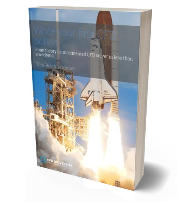
Join the CFD community with over 1,000+ like-minded people and get a free ebook that walks you through writing your first CFD solver in less than a weekend, even if you've never written one before. I'm not a big CFD corporation, just a passionate developer and academic who clearly has too much time. I won't spam you, and you can unsubscribe at any time.

This series explores a collection of libraries that will make writing CFD solver easier, faster, and more fun.

If you are new to CFD, start here. This series covers all the key concepts you need to become a CFD expert, from A to Z.

This series teaches you how to automate compiling, linking, dependency management, testing, and installation of your CFD solvers and libraries with CMake.
I do! And I love CFD. Hi, I'm Tom, I am a former CFD software developer and now a senior lecturer in Computational Fluid Dynamics at Cranfield University (UK).
I wrote my first CFD solver in 2012; since then, I have written many more, and I have worked on a commercial CFD solvers as well as on open-source and in-house CFD codes.
When I learned about CFD, the textbooks that were available to me mostly talked about equations (with very little explanation), and I was struggeling to put these equations into code.
I eventually managed to get my solvers to work, and when I did, I started to develop a deep and intuitive understaning for CFD.
I can't be the only one who wants to understand CFD in-depth, and so, this is why I have created this website, to help you learn in minutes what took me years to master.
If you are new to CFD and interested, I hope that this website will give you the theoretical and practical understanding you need to master CFD, which goes beyond the class room and classical textbooks.
This website was created on a sleepless night in May 2023. It was 4am, I went downstairs, sat down, wrote my first article, and I haven't stopped writing since.
If just one person finds the writing helpful, then it was all worth it. Thanks for stopping by!
All the best,
Tom

Do you want to learn how to put the Navier-Stokes equations into code and write your own solver?
Sign up for my newsletter, and you get my eBook Write your first CFD solver - From theory to implemented CFD solver in less than a weekend for free!