The complete guide to linear system of equation solvers (Ax=b) in CFD
In our series thus far, we have looked at how to derive the governing equations of fluid mechanics, we have discretised them, and we have looked at numerical schemes to solve our discretised terms, with different orders of approximation and stability.
When we discretised our equations using an explicit time integration, we saw that we get very easy to implement discretised equations, but we are limited by the CFL condition, which restricts the timestep at which we can advance our solution in time. For scale-resolving turbulent simulations, this may be OK, as our time step may be limited by physical processes.
In general engineering, however, we replace turbulence by RANS models and want to obtain solutions to complex problems in as little time as possible. The only way to do this is to use an implicit discretisation, where we have no limit on the CFL condition, and we can march our solution to convergence as quickly as we would like.
All implicit equations have one thing in common: We have to solve a linear system of equations of the form , where is a coefficient matrix which is constructed from the equation we are solving, as well as the numerical schemes we use to discretise our equation. is the solution vector we are solving for and contains any non-implicit contributions, as well as boundary conditions.
In this article, we will first develop a unified view for how we can write any explicit and implicit equation as a linear system of the form of . We will then look at the properties that are important when we want to solve . With that knowledge in mind, we will go through and derive classical methods to solve these systems, starting with Gaussian elimination and the LU decomposition, and we will look at why these methods aren't really useful for CFD problems.
We then venture into the methods that are actually used in CFD: starting with matrix-free methods like the Jacobi and the various Gauss-Seidel forms, we see how they can solve the system effectively, but with a high computational cost. We then peek inside the Krylov subspace and see that we can find a solution to with relative ease by reformulating this problem into a geometric problem, where represents a surface on which we want to find a minimum.
Specifically, we will look at the method of Steepest Descent, as well as the family of the Conjugate Gradient algorithms (Conjugate Gradient, Bi-Conjugate Gradient, and Bi-Conjugate Gradient Stabilised). As there is no proper derivation of these methods in the literature, you'll find one here.
This discussion is augmented by preconditioning to even further reduce computational costs, as well as a completely different approach known as the multigrid approach, where we focus on smoothing errors, rather than solving directly. We do solve this linear system at some point, but for the most part, we are working on the error, and a full derivation for that is, of course, also provided.
Now, this is a long piece of text, likely requiring a few sittings to go through it, but if you want to know how a real CFD solver works under the hood, there is no way around these topics. Any CFD solver you will either have worked with or will work with in the future will have the methods implemented that are mentioned in this article.
Bring a strong cup of tea; you will need it. Are you ready to go?
In this series
[custom_category_posts_list category_slug="10-key-concepts-everyone-must-understand-in-cfd"]
In this article
- Introduction
- Direct methods
- Matrix-free methods
- Krylov subspace methods
- The multigrid approach
- Preconditioning
- Extension of linear system of equations solver to non-linear systems
- Summary
Introduction
I have a confession to make. For the longest time, I have avoided linear systems of equations like the pest. Even when I had to solve them, like the Pressure Poisson equation, I used whatever method was quickest to implement, without giving much thought towards convergence properties or performance. I was very happy to wait for a month for the simulations to finish, and I was living a happy life without matrices in my life.
I think this has to do with my (professional) upbringing; as a student, you are very impressionable, and one thing I often heard is that linear system of equations solvers, i.e. those that solve , are, well, linear. The governing equations of fluid mechanics are non-linear, and so, the reason was that, as we have to linearise the system of equations, we are losing some non-linearity.
Well, this is true, but we are able to recover the non-linearity through an iterative procedure (something which we will touch upon at the end of this article), and while it will cost additional iterations, the convergence rate that you will obtain from solving usually offsets this additional cost.
In this article, I want to give you an introduction to methods to solve that I was always lacking. The combination of fearmongering by some of my professors and the sense of comfort explicit methods gave me meant that I never really felt compelled to look into implicit systems in earnest. But once I did, I regretted having waited for so long.
In this article, I want to equip you with all the necessary knowledge so that you can integrate implicit solvers, i.e. those that solve , into your CFD codes.
Before we jump into all of the various methods to solve , let us first look at how this linear system of equations comes about, and then we will look at methods to solve it!
A unified view on how Ax=b is constructed and solved
In the following, I want to give you a unified view on how is constructed. I haven't seen this written anywhere (perhaps it is and I just haven't seen it), but after I saw linear systems from this unified perspective, I felt that I had a much better and deeper, intuitive understanding of how to construct explicit and implicit time integration schemes.
To start us off, we need to talk about explicit and implicit time integration. An explicit time integration scheme is one where, after discretisation, only one unknown is left in the discretised equation. We can solve for this unknown explicitly. Conversely, an implicit time integration scheme is one where, after discretisation, more than one unknown is obtained, and we are only able to solve this through a linear system of equations, i.e. by solving .
Let's take a simple, 1D equation to see what I mean. Let us discretise the following unsteady heat-diffusion equation:
Let's discretise that with a simple first-order Euler method in time, and a second-order central scheme in space. We will denote the unknown (next) time level by , while all variables at the current time level are known. Therefore, we obtain the following equations:
- Explicit time integration:
- Implicit time integration:
We see that the only difference is at which time level we evaluate the temperatures on the right-hand side, i.e. either at or at . The next step is to collect all unknowns on the left-hand side of the equation, all knowns on the right-hand side of the equation, and then to write the equation in coefficient form. This is done in the following way for both schemes:
- Explicit time integration:
- Implicit time integration:
A common notation here is to introduce coefficients , , and for the coefficients in-front of , , and , respectively, with and standing for east and west. Furthermore, all of the known quantities on the right-hand side can be put together into a single value, which we will denote as . Doing so gives us the following system of equations:
We can then write the coefficients as:
- Explicit time integration:
- Implicit time integration:
Since this Eq.(6) is given in terms of , we will obtain this equation for each node in our mesh. So, if we have nodes in our 1D mesh, then we will obtain Eq.(6) for 5 different nodes.
We have to take special care at boundaries, that is, how we impose values on the left and right sides of the domain. We can either impose Dirichlet, Neumann, or Robin boundary conditions, and how to do that, including for linear systems like the ones we are currently looking at, is the subject of the next article on boundary conditions.
Let's say we want to impose Dirichlet boundary conditions on the left and right side of the domain; that is, we want to impose a fixed temperature on the left and right sides of the domain. Let's say we set the temperature to on the left boundary of the domain, and on the right boundary of the domain. If we want to do that, the trick here is to set and , as well as and . To make this clear, on the left side of the domain, at the boundary, we impose:
On the right side of the domain, we have:
If we insert these values back into Eq.(6), we obtain (now using to write the equation for both left and right sides of the domain):
I have gone over this a bit quickly, but I have a much more in-depth discussion for how to apply these types of boundary conditions in the next article in the section How to implement boundary conditions for implicit time integration. Give that a read if you want to have a more thorough explanation.
With these boundary conditions defined, we can now write all of the equations, for each node , in matrix form, that is, we can write what we have just discretised as . Let's stay with the example of using 5 nodes. This means we have 2 nodes on the boundary and 3 nodes on the internal domain. A sketch of this domain is shown in the following:

For the 1D domain, noting that , we can now write our linear system as:
We can now insert values we have for our coefficients , , and , as well as for the right-hand side vector . For the first and last row, we have to apply our boundary conditions, that is, , , and . This is true for both explicit and implicit time integrations. Let's do this now. For both explicit and implicit time integrations, we obtain the following linear systems of equations:
- Explicit time integration:
- Implicit time integration:
To see that this really does represent our original equations, you can take any row in the coefficient matrix, multiply that by the solution vector , which represents the temperature in our example, and set that equal to the right-hand side vector . For example, taking the third row in both cases results in:
- Explicit time integration:
- Implicit time integration:
I have given both versions here, i.e. with explicit indices , and with . If we can now make the mental substitution of , then we see that the above equations really are the same as Eq.(4) and Eq.(5).
OK, so now we need to solve our linear system of equations. From linear algebra, we know that we can solve by inverting the coefficient matrix and then left-multiplying it with the equation, i.e.:
Here, is the identity matrix, i.e. containing ones on the main diagonal and zeros everywhere else. Let's look at the explicit time integration case first. Our coefficient matrix is:
Since we only have elements on the diagonal, we can easily invert this matrix with the following rule:
Here, are the entries in the inverted matrix, i.e. at row and column . Since both row and column indices are always the same, we will always pick the value on the diagonal. The values of are coming from the diagonal of the original coefficient matrix . With this rule, we can now invert the coefficient matrix as:
We can also write our discretised system for now as , this becomes:
Again, taking the third row as an example, we can write out the discretised equation as:
Again, if we can mentally replace in this case, then we realise that this is really just Eq.(2), which we saw at the very beginning. We can easily rearrange Eq.(2) to look like Eq.(22). So, all of this discussion of bringing Eq.(2) into the form of , inverting the coefficient matrix, and then solving for seems a bit over the top, doesn't it?
Hold on to that thought, we will be coming back to that in just a second! But, before we do, let's also look at the implicit time integration case quickly. Here, the coefficient matrix was given as:
In this case, we have elements both on the diagonal and on the off-diagonal. Because of these off-diagonal entries in , we can no longer find the inverse, i.e. , in the same way as we did with the explicit time integration case. Thus, we are forced to compute it properly, and, as it turns out, once we have large systems, this becomes impossible.
Just to bring home this point: The number of nodes or cells in your mesh determines the size of your coefficient matrix. If you have 1 million cells in your mesh, your matrix will have 1 million rows and columns. Inverting a 1 million by 1 million matrix, even if most of the entries are zero, is essentially impossible, and we have to potentially do that at each timestep and/or iteration.
To add insult to injury, 1 million cells, in the context of CFD, is a pretty small simulation. You may have some simple test cases that have only a few hundred thousand cells. For example, a classical 2D airfoil simulation will probably have about 100,000 cells. But any 3D engineering applications that are of industrial interest can easily reach the hundreds of millions of cells. In one case, I am aware of a company routinely running 1 billion cells per simulation.
If you are planning to write a CFD solver for these types of applications and you propose to invert the matrix at each iteration, I think you may be shot. Don't know, but that feels about right. Don't do it.
There are now essentially 2 things we can do: either we try to numerically approximate the inverse of , or we just try to find a corrective algorithm that will try, starting from some initial guess , to find a solution that satisfies our original system of equations . Typically, we do the latter.
The rest of this article is essentially dedicated to exploring these methods, which find the solution of in an iterative procedure. These iterative procedures mainly differ in their approach to solving the linear system, but some are better than others in terms of convergence and stability.
Thankfully, we have a lot of experience with all of these different methods, and while the literature is filled with all sorts of different algorithms, there really are just a few that we need to know about. These are the ones you will find in actual CFD solvers. All of the other methods may have some relevance outside the field of CFD, but we do not need to take a great interest in them.
Before we start looking at some matrix properties, I wanted to come back to my unified view, which I was telling you about before. I showed you that both explicit and implicit time integrations can be represented as . Typically, when we write an explicit solver, we would probably not write the explicit system in this form, simply because it takes more lines of code and complexity.
But there is one very important reason why I would encourage you to even write your system like that. If you do, you can use any matrix vector library that will do all of the computation for you. That, on its own, may not be necessarily an advantage, but if that library offers parallelisation support, you can use that without having to think about parallelising the code yourself.
And, if you do decide to support implicit time stepping at some point in the future, well, the infrastructure will already be there in your code; you just have to rederive the system of equations for that particular discretisation. Well, even that can be automated by packages like Sympy, Maple, or even Matlab's symbolic toolbox.
Hopefully, this makes sense. So, if you see , just know that this really represents the governing equation you are trying to solve. Change the coefficient matrix or the right-hand side vector , and you solve a different equation. With that out of the way, let's start looking at some matrix properties.## Matrix properties
At this point in the discussion, we have to talk about matrices. If you just think of them as a 2D storage container, oh boy, you are in for an awakening. People have filled entire books about matrices alone. Believe me, people have made a lot of effort trying to study and demystify matrices. So, in this section, we will look at some of the their properties.
Dense and sparse matrices
Let's start off easy and look at the two structures a matrix can be in. A dense matrix is one in which all, or almost all, entries in the matrix are non-zero. In contrast, a sparse matrix contains mostly zeros, where typically only the diagonal and some off-diagonals contain non-zero entries. The off-diagonals are shifted from the diagonal of the matrix either to the right or down. The following sketch shows this, where a cross indicates that this entry is a non-zero value.

If we go back to our example in the previous section, we had the following matrix for the implicit time integration:
This matrix contains elements only on the diagonal (either or ), while the two off-diagonals contain the entries . So, this is a sparse matrix, and all of our matrices that arise in CFD (as part of discretising our governing equations) will be sparse. Sparse matrices themselves are a topic you could do an entire PhD on (if you were that committed), and we will touch upon some key properties in a second.
Lower and Upper triangular matrices
In the analysis that will follow, we will make heavy use of lower (L) and upper (U) triangular matrices. If you already know, or have heard, of the LU decomposition, that is what the letter stands for.
Since we can add matrices together, that means that we can decompose them into as many matrices as we want. A common decomposition is to split a matrix into its lower, upper, and sometimes also diagonal parts, as shown in the following sketch for a dense matrix:

We can thus say that if we are dealing with a matrix , we can write this matrix as well:
Sometimes, we write this decomposition simply as:
If we do that, then the diagonal matrix has been either absorbed into the upper or lower triangular matrix.
Symmetric and non-symmetric matrices
Now that we can decompose our matrix into its lower and upper triangular matrix, we can easily check if our matrix is symmetric or not. A symmetric matrix is one where all the elements are mirrored along the diagonal of the matrix. That means that if I have a matrix entry , the coefficient in a matrix at row 2 and column 4, it will be the same as , i.e. the coefficient at row 4 and column 2. We can generalise this as .
Since the transpose of a matrix is essentially just flipping a matrix at its diagonal, we can say that the transpose of a symmetric matrix is just the matrix itself. In mathematical terms, we can write:
And, since we have introduced the decomposition into the lower and upper triangular parts already, we can also look at what happens if we transpose either the lower or upper triangular matrix. In this case, I refer to the lower and upper triangular matrices which do not contain the diagonal, i.e. the is treated separately.
If we take the lower triangular matrix and transpose it, we flip it at the diagonal. So it will now occupy the space where the upper triangular matrix is. If the matrix is symmetric, then both of these will have the same values, i.e. the transpose of the lower triangular matrix is the same as the upper triangular matrix. The same is true for the transpose of the upper triangular matrix, which is the same as the lower triangular matrix. We can write this as:
How matrices are stored
For a dense matrix, we do have to store the entire matrix, i.e. each coefficient . There is no way around that. For small problem sizes, that isn't a problem, but consider that a matrix will have entries. The matrices that we will look at will all be square matrices, so . This means that our matrix will contain entries. So, if I have a mesh with 10 cells, my matrix will contain entries. If I double the number of cells to 20, then my matrix will contain .
Thus, the number of elements we have to store grow exponentially (to the power of 2), and if we are dealing with 1 million elements in our mesh, well, we have to store . We don't do that, especially if our matrix is sparse. If we had a sparse matrix which contains one diagonal, and, for the sake of argument, let's say we also store 6 off-diagonal entries. Then, we store entries in the diagonal term, and a few less in each off-diagonal.
If we look back to our dense vs. sparse matrix sketch above, we saw that the diagonal in the sparse matrix contains 8 entries, while there are two off-diagonals that contain 7 entries and two off-diagonals that contain 4 entries. So, the further the off-diagonals are away from the diagonal, the fewer entries they will have, but in our example, if the off-diagonals have a few elements missing compared to the diagonal (which has entries), then they will still have close to entries.
Let's just assume that each off-diagonal also stores . Then, we store one diagonal + 6 off-diagonals, so entries in total. If we stored that in a dense matrix, where each zero would be stored as well, we said that we would be needing to store entries. If we take the ratio, then we can estimate how many elements in that matrix will actually be non-zero. We have:
So, we only need 0.0007% of the matrix; the remaining 99.9993% are just zeros. For this reason, we really want to store sparse matrices in a different form, not as a full, dense matrix.
There are a few different forms for how we can store sparse matrices, and conceptually, the easiest to understand is the coordinate matrix, as shown in the following image:
We need to store the row, the column, and the value at this location. We do that by storing all of this information in three separate vectors. If we are now evaluating a matrix vector product of the form , where is the matrix and is a vector, then we will have to multiply each row of with the full vector . If we say that we count rows with index and columns with index , then we can say that each row will perform the following computation:
So, if we wanted to evaluate this with a sparse matrix, which we store in coordinate form, we would have to check, for each row, if any values are actually stored. So, referring to the figure above, if we are in row 5, we see that there are no entries here. There is also no 5 in our row vector, as shown to the right of the matrix. Thus, we can say that, since there is no data here, the result of the summation in Eq.(30) is zero.
However, if we go to row 3, for example, then we do have a value at column location . Since we start with a zero index, corresponds to the fifth column, and so we have to multiply this by the fifth entry in the vector , i.e. .
So, when we evaluate Eq.(30), we have to check now, for each value , if it exists. If it does, great, we can perform the computation. If it doesn't, then we set . In reality, we would implement the summation as shown in Eq.(30), though, as this would be very wasteful.
Let's go back to our previous example of the 1 million by 1 million coefficient matrix. Here we said that we had entries. So, we would not be checking times if an entry existed, that would be just as bad as storing the matrix itself. To make this clear, let's look at the example of evaluating .
To make this a concrete example, let's use some numbers. I will be using the same matrix as shown above in the figure, but I have come up with a very creative vector, if I may say so myself, that we'll use to multiply our matrix with (i.e. the vector ). The resulting vector can then be calculated as:

Look at Eq.(30) again, for each row in the vector , we have to sum over all of the products of and , where the coefficients in are non-zero. For the first row, we see that the third column has a non-zero value of 9, so we multiply that by the third entry in , which is 3, and so the corresponding product is . We add that to at the first row.
Since we do not have any additional coefficient in in the first row, we do not add anything else to in the first row. Well, this is just matrix vector multiplication, hopefully this is something you have heard before. And if not, you must be a child under the age of 18.
I recently had to update my privacy policy, and I used one of those privacy policy generators, that asks you a few questions and then customises the privacy policy for you. I looked through it, and according to that privacy policy, children (which were counting as those that are under the age of 18), are not allowed to consume the content on this website.
Well, what harm is there in a 17-year-old, a day away from their 18th birthday, to learn about matrix-vector multiplication, I ask? I didn't quite see the point. I removed that paragraph and now anyone from the age of 0-99+ is allowed to consume my content to their heart's content. You are welcome.
In any case, now that we have an example, let's implement that into code. I have written a small Python script that will do this for us. Have a look through it, I'll explain it below if it is not clear.
1 2 3 4 5 6 7 8 9 10 11 12 13 14 15 16 17 18 19 | # coordinate matrix form rows = [1, 3, 0, 2, 4] columns = [1, 4, 2, 3, 3] data = [2, 5, 9, 1, 6] number_of_non_zero_elements = len(data) # vector b, which we use in matrix vector multiplication b = [1, 2, 3, 4, 5, 6] # result vector c, which is initialised to 0 everywhere c = [0, 0, 0, 0, 0, 0] for i in range(0, number_of_non_zero_elements): row_id = rows[i] column_id = columns[i] c[row_id] += data[i] * b[column_id] print(c) # this prints: [27, 4, 4, 25, 24, 0] |
First, we are going to set all values in to zero. This is important, as we will be adding results to this vector now, and we may be adding more than once to the same location in . Then, we will loop over the number of elements in the coefficient matrix . If we look at the example calculation above, we had 5 entries in total in , so our loop length would be 5 (number_of_non_zero_elements), and not , which is the size of the matrix shown (with 6 rows and 7 columns).
Then at each loop iteration, we get the current row, the current column, and the value at that location. We now also get the value in our vector, specifically at the same location as our column location that we got from our matrix. We multiply these values together, and then add to , specifically at the same row location we received from the matrix. We need to add this value to whatever was previously stored in this vector, since we may have more than one value per row stored in .
As you can see, the results that are being printed are the ones we would expect. Now, this is a quick and dirty example, by just hardcoding the rows, columns, and data entries, but we could also make this a bit cleaner by creating a CoordinateMatrix class, which stores these arrays. If we then overload the multiplication operator, i.e. the * operator, then we could write our matrix vector product as c = A * b. Wouldn't that be nice? Well, that isn't really a big issue in Python, and we could achieve this by writing:
1 2 3 4 5 6 7 8 9 10 11 12 13 14 15 16 17 18 19 20 21 22 23 24 | class CoordinateMatrix: def __init__(self): self.rows = [] self.columns = [] self.data = [] def __mul__(self, b): c = [0] * len(b) for i in range(0, len(self.rows)): row_id = self.rows[i] column_id = self.columns[i] c[row_id] += self.data[i] * b[column_id] return c A = CoordinateMatrix() A.rows = [1, 3, 0, 2, 4] A.columns = [1, 4, 2, 3, 3] A.data = [2, 5, 9, 1, 6] b = [1, 2, 3, 4, 5, 6] c = A * b print(c) # prints [27, 4, 4, 25, 24, 0] |
If this makes sense, then congratulations, you have mastered the most difficult bit already about sparse matrices and how we store them. However, the coordinate form is not as efficient as some other sparse matrix storage formats, and so we don't actually use this format in practice, at least not for the actual matrix vector multiplication.
The format you will most likely use when you are dealing with sparse matrices is the compressed sparse row, or CSR format. Now, I did already talk about the CSR format in depth in my article on sparse matrices in CFD application, which you may want to consult. In that article, I also show how we can implement this format into a C++ code. But I want to give a brief overview here as well, so that you understand the basic concept.
The CSR format is conceptually very similar to the coordinate matrix form (sometimes also abbreviated as the COO form). The following figure shows how we store a matrix in CSR form:
We have again three arrays that we are storing, but we store different information here. Arguably, the information that we do store is organised in a way that isn't as clear as the coordinate form, and there are good reasons for it. So, let's look at this storage form and then discuss why this is better.
First up, we have the index pointer array, and it has the same length as the number of rows + 1. We will get to this array in a second. We also have an indices array, which will give us the column indices of where values are stored, and then we have a data array again, which stores the actual non-zero values.
OK, so we have a indices array, which will give us the column index, but where is the array giving us the corresponding row entry? Well, it is encoded in the index pointer array. The index pointer array, we said, had a length of the number of rows + 1. We can use this fact and say that if we want to get some information about, say, row 0, or 4, all I have to do is to go into the corresponding location within the index pointer array.
OK, so let's do that. At location 0, within the index pointer array, we have a value of 0. We also need to get the next entry in this array (and for that reason, this array has one additional entry compared to the number of rows), which is 2. The location in the index pointer array that we access, in our case, was the first location (i.e. index 0), that corresponds to the first row (again, with index 0). So whatever information we are reading will be relevant for row 0.
We read the value at location 0, plus the next entry, and we got the values 0 and 2 from the index pointer array. The difference between the two is . This tells us that there are 2 non-zero elements for row 0. We can see that this is the case from the figure above. So, we already know that we are in row 0; now we need to get the column locations (or indices). This is where the indices array comes in.
The index pointernot only tells us how many entries there are in the corresponding row, but it will also give us the indices we have to use to get the column locations from the indices array. Which indices did we read? Well, we know that there are 2 non-zero elements in row 0, and, the index pointer at location 0 is 0 as well, so it tells us that we have to go into the indices array at location 0 (this is what we read from the index pointer array), and then we have to read 2 entries from this array.
These two entries in the indices array are 0 and 2, so we know that in row 0, there are two non-zero elements at columns 0 and 2. We can again confirm that this is correct from the figure above. We do the same trick to retrieve the non-zero values from the data array, i.e. we go to location 0 and read the next two entries here, which are 8 and 2. So, we know that at row 0 and column 0, we have a value of 8, and at row 0 and column 2, we have a value of 2.
Let's do that again for location 4 (i.e. the fifth entry) in the index pointer array. So, for row 4, we get index pointer[4]=3. The next entry in the same array gives us index pointer[5]=6. This means that there are 6-3=3 entries in row 4. Thus, we have to go into the indices array, at location 3, and then read the next three values, which will give us the corresponding column indices/locations.
If we do that, we get indices[3]=2, indices[4]=3, and indices[5]=4. The corresponding non-zero values are data[3]=7, data[4]=1, and data[5]=2. Looking at the figure above, we can again see that this is correct.
Well, if we look at this format, we may be asking, why is this so much better than the coordinate matrix format? Well, for starters, we no longer store the row index explicitly. So we have already reduced the storage requirements somewhat. I'd argue that this is not really that much of a problem, for the applications that we have in mind (CFD), the coordinate format would require, perhaps, 50% more storage. So, yes, it would be larger, but not that much. If performance is our main driving force, though, CSR is an easy optimisation.
In any case, there is a much bigger advantage for CSR. In the coordinate matrix form, we were not required to store the non-zero values in any particular order. This is very lucrative when we are building the matrix, and we don't know yet exactly how our sparse matrix will look. So we can always easily append a row and column index with an associated non-zero matrix coefficient, and it doesn't matter in which order we append that.
We saw from our coordinate matrix example before that there wasn't any particular order in which the rows were stored. For the CSR matrix, though, the storage order is important, and we have to store all values row-by-row. This means that when we get data from RAM and load that into our CPU, all values that are stored in one row will likely be within a cache line. As a result, when we perform the matrix vector multiplication, we will have fewer cache misses and so overall faster computation of our matrix vector product.
If you want to see how to implement sparse matrices using the CSR format, you can check out the implementation, as well as some additional thoughts on the CSR format in the sparse matrices in CFD application article.
Some libraries that compute sparse matrix vector products may actually allow you to first assemble your matrix as a coordinate matrix (which means you can easily add non-zero values at arbitrary locations). Once you are done, the library may then lock the matrix and transform it into a CSR format to make it more memory efficient. So, the coordinate matrix is still useful, but for performance reasons, we prefer CSR.
I hope you can see now why we really want to store sparse matrices in a different format. If you understand both the coordinate and compressed sparse row format, you know the most important ones. There are other formats available, but they essentially do the same thing; they may just store different arrays and thus retrieve data differently.
The Krylov subspace
If you are designing websites, it is customary to select a primary colour and a secondary colour for contrast. These are the only colours you will then use throughout the entire website design. Combine that with a background colour, and you have everything that you need. Can you guess which primary colour I have picked? While this website is now much more toned-down, it used to be a lot more aggressively pink (mainly because I used wordpress and I just couldn't figure out (or couldn't be asked?!) how to make the website, well, less pink).
In my case, I have settled for a cold, dark blue, but you may read this in the future where I have changed my mind again and adopted a tropical colour scheme, who knows. Next time you visit a website, look out for the primary and secondary colour (there is no real secondary colour on this website, at least not in the version that was live when I wrote this).
So, if we pick any colour from the rainbow of colours, we can form a subset of colours. In my case, this website uses the subset of colours which are white, dark grey, and dark blue. But we can pick any other colours as well; there is no limitation on what we can pick, apart from the colours having to look good together.
Contrast a subset now with a subspace. A subspace is similar to a subset, but if I combine two elements from a subspace, I do get a different element that lives in the same subspace. So, if we go back to our colour example, a subspace of colours would be any shades of a specific colour. So instead of settling, for example, only for the colour of blue, I could select shades of blue, which would form both a subset and a subspace.
If I combine two shades of blue, I get another shade of blue. I can repeat this process with any shade of blue, and I will always get some form of blue back. Now, if I throw in the colour green, I will lose my subspace. Blue and green will give me a different colour when combined; it will no longer be purely blue. However, blue and green still form a subset of all the colours.
So, a subset can be any set of a larger collection, and there really aren't any rules. Anything is allowed, much like the very liberal choices my neighbour makes about her clothes. I'd argue a towel is not a subset of clothes that can be worn, but she has invented the towel one-piece no one has asked for (and, my window blinds are permanently shut as a result).
A subspace, then, is like a subset, but with some rules or structure. In this case, a combination of elements within a subspace needs to produce a new element in the subspace. Let me give you a different example, which is a bit more mathematical. Let's look at the following vector:
If I asked you to produce two vectors, at random, you may give me:
Excellent choice, really putting your creativity here on display. Let's see what happens when we add these together, i.e. we compute . We get:
Did you notice something about these vectors? Both and are, first of all, subsets of all the vectors in three-dimensional space. Mathematically speaking, we can say that and are part of (the three dimensional space), or . If we want to say that and are a subset of , then we would write:
But, and do not just form a subset, they also form a subspace! Both and have , that is, the third component of the vector is zero. Since both vectors only contain and elements, we can say that both and live inside the xy-plane. And, what happened when we added and together? The resulting vector was also part of the xy-plane.
Thus, and are not just a subset, but they are also a subspace! Let's look at them for a moment:
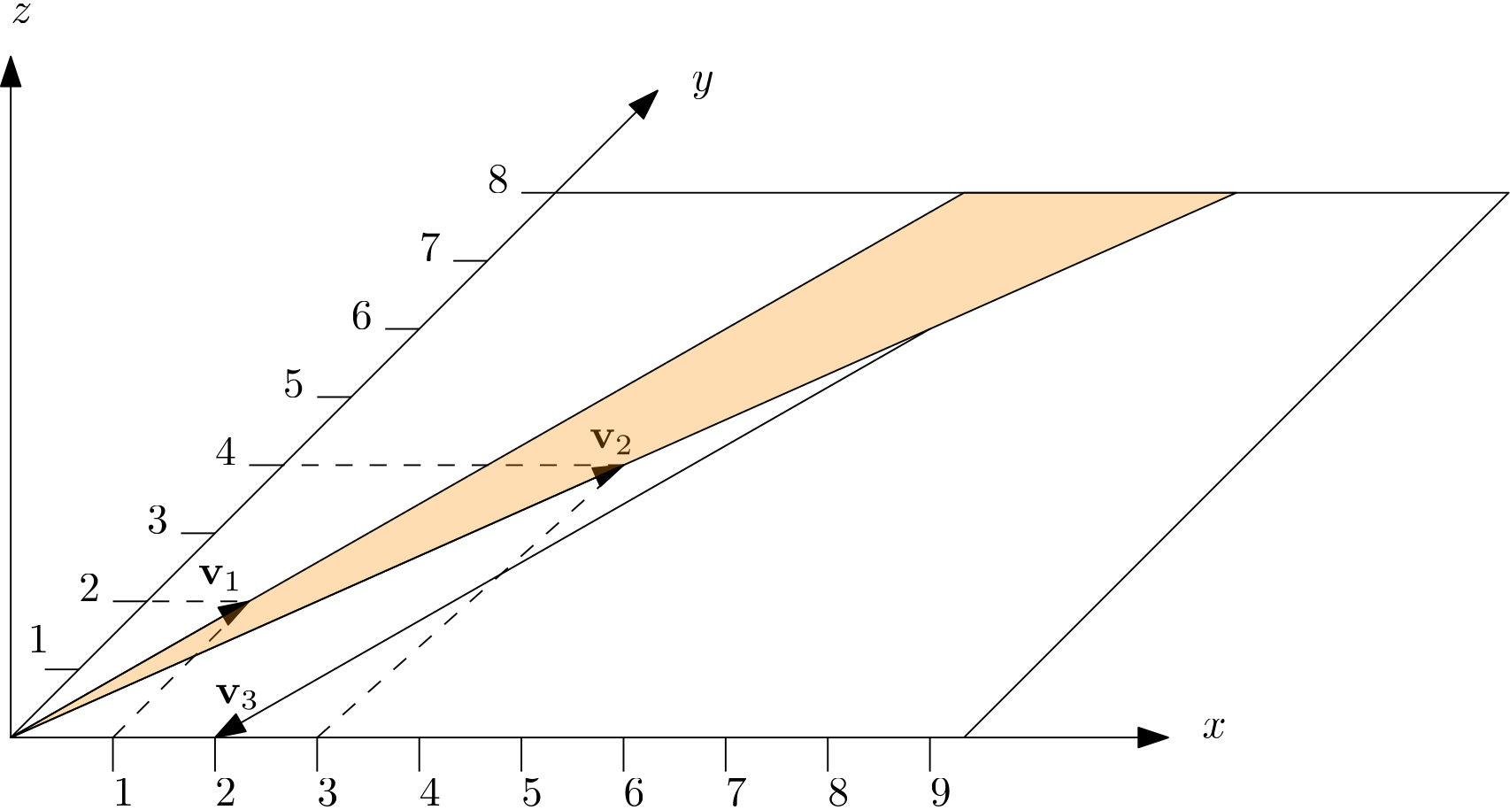
We can see that both and are indeed in the xy-plane, and we can see that they span the area shown in orange. Does this mean and only form a subset of the subspace (i.e. we can only reach the parts shown in orange)? Not quite. As long as two vectors are linearly independent, we can reach any point in the xy plane!
We can see that both vectors are linearly independent in the figure. If they are not linearly independent, then they would both point in the same direction. For example, a vector with coordinates and another vector with would not be linearly independent. If we divide the second by 2, we get the first vector, so they are linearly dependent.
Let's show that and are linearly independent. We can create any vector in the xy plane as a linear combination of and as:
For example, with and , we have:
We can see this vector in the figure above, and we can confirm that this vector is not just part of the orange area, but indeed outside it. Thus, using and alone, we can form the entire subspace, i.e. we can reach any point in the xy plane. We just have to find the values for and , that's all.
Mathematically speaking, we can write this subspace as:
Here, the span keyword states that and form the entire subspace. As we saw, we can reach any point in the subspace as a linear combination of these two vectors. The right-hand side states that any real numbers () and form a vector , which is part of the three-dimensional space .
Let's step back and see why this subspace definition is important. Let's say we want to draw a map of a city. The city exists in three-dimensional space, and some cities will have rather large elevation changes. So, we could draw an isometric projection of the city, show all of the elevation changes, as well as the city itself. But that's not what we normally do, is it?
Instead, we can say that we project the entire 3D city onto a 2D subspace, and then we draw the city here. This simplifies our task to draw the city on a 2D piece of paper. So, certain tasks become easier in a subspace.
With this in mind, let us now turn to the Krylov subspace and why this is so important. Imagine the following scenario: You and your friend have reached fame beyond your wildest imagination, and you are making a trailer for your new and upcoming show. You both decide that jumping out of an airplane with a parachute would be a good idea, and then doing the promotion while falling through the sky. The twist: Your friend decided to prank you.
One by one, people jump out of the airplane as planned. But then, the pilot comes up to you and says, "Your friend told me you always wanted to be a pilot, have fun!" and then he jumps out as well. You are left on your own, and you have no idea how to fly a plane. Sounds a bit far-fetched? This actually happened in Germany. If you want to see what happened, see here: Part1 and Part2 (you may want to use auto-generated subtitles/voice-over). As they say, German sense of humor ...
But let's put ourselves in the same position. We have no idea how to fly the airplane, but we need to learn how to fly it, and fast! What would you do? Well, we humans are incredibly good at observing things and drawing conclusions. So, our natural instinct is to manipulate an unknown system and then see how this system responds. In this case, the unknown system is the aircraft, and so a sensible thing to do may be to push the controls forward and to pull them back to see how the aircraft responds.
We notice that pushing the controls forward, the aircraft starts to lower the nose, and we start to lose altitude. As we pull back on the controls, the aircraft raises the nose again, and we increase in altitude. So we have recorded two responses of the system based on our inputs. Let's now formalise this. Let's say that we have a state vector that stores our input. Let's call this vector . So, we push or pull the controls, and this will change the inputs to the vector .
This vector stores the pitch (pulling or pushing the controls), the roll (turning the aircraft left or right), and the yaw (also turning the aircraft left and right but with the rudder pedals). From flight dynamics, we know that equations do exist which describe the motion of an airplane based on changes to its state (roll, pitch, and yaw). But let's say we don't know that.
However, as we saw at the beginning of this article, we can write any equation as a matrix vector product of the coefficients from the equation and the independent variables, e.g. roll, pitch, and yaw. See Eq.(12), for example, where we wrote our partial differential equation as a matrix vector product. So, we can conclude that if we have a vector containing roll, pitch, and yaw, we can multiply that by some matrix , which will then give us the response of the aircraft.
So, we pull back on the controls (we change ), and, as we already discussed, this results in the aircraft pitching the nose up. Thus, , that is, the response of the aircraft to changes in our inputs, is that the nose is raised and we start to climb. Now, here comes the next part, and this is critical. What happens to the aircraft when we are in this state of having a raised nose?
Well, if we release the controls, the aircraft will lower the nose by itslelf and go back into a state of equilibrium, this is just how aircrafts are designed (except for military jets). How can we express that in mathematical terms? We said that raising the nose and gaining altitude was a response from our aircraft as a change in , so we recorded that as . The response of the aircraft to this state is, well, . So, we check the response of the aircraft to a state in which we brought it before.
We can also write this as: . What happens next? So, we have raised the nose, which was our input . Then, we released the controls, and the aircraft started to pitch down again. This was the aircraft's response to our input, and this was . And now, the aircraft will initially pitch down a bit too much, and so we will actually start the descent. This is the aircraft's response to its own previous response to our change in control input.
We can write this as . It will now pitch up again, so it is the response to the previous state, and this could be captured as , and so on. This motion is known as the phugoid, and it is shown in the following figure:
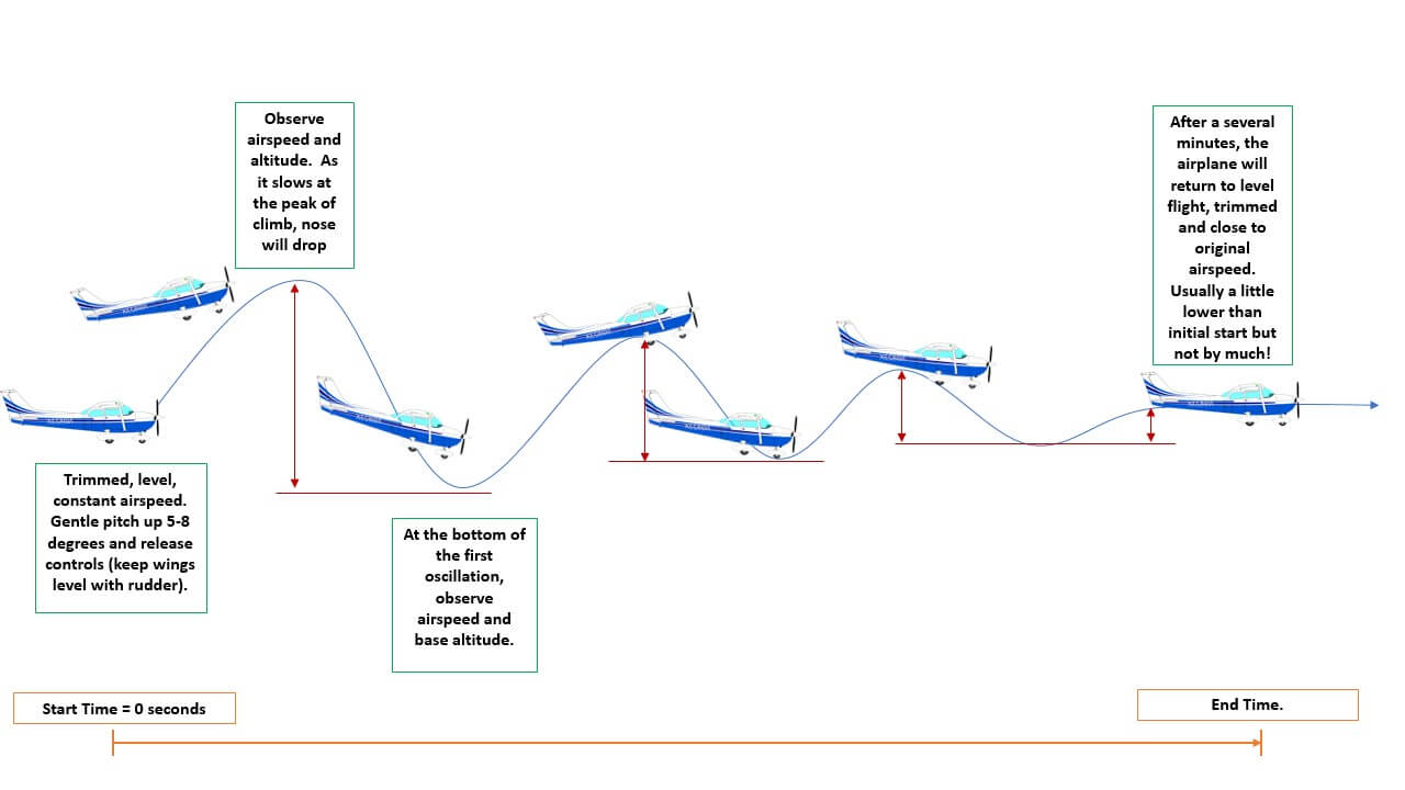
One of the perks of working at a university with its own airport (and its own set of research aircraft) is that we do get to fly these types of manoeuvres, and it never gets boring! Depending on your weight and balance, you can either fly a stable or unstable phugoid (where the oscillation is damped or amplified). In both cases (but in particular in the unstable mode), you get close to 0g, something which is best experienced and difficult to describe.
In any case, let's take a step back, again, and see what we have done. We have played with the controls, and we have gotten a sense for how the aircraft will react to our inputs (), as well as to its own inputs, i.e. those states produced from our initial input (). We can do the same thing by turning the controls, pushing the rudders, changing the throttles, pressing buttons, etc. and then record what happens.
All of this will help us understand how the aircraft behaves. That is, we don't know anything about the internal working of the aircraft (we don't know the matrix ), but we can test how the aircraft responses to our inputs (we can observe what the results are of and subsequent reactions of the aircraft ).
Thus, our input and all of the multiplications with form a subspace that represents how our aircraft responds. The matrix is just a normal matrix, but not all matrices are part of the subspace in which the responses live. For example, if we allowed any matrix to be part of the subspace, that means that we may pull back on the controls, and instead of raising the nose, we now operate the throttles with the controls.
This is not an expected behaviour, but if we did not have a subspace, i.e. if we said any matrix can be used here, then we would get random and unexpected behaviour. Earlier, I said that a subspace has a certain structure, which differentiates it from a subset. The structure here is that changes to our pitch will always result in either nose up or nose down, but it will not suddenly operate the throttles, or the radio, or the windscreen wipers, etc.
Just for completeness, changes in pitch can, under certain circumstances, result in roll as well (pitch and roll are coupled in reality). If we fly near the stall speed, one wing may stall before the other, leading to a loss in lift on one side and an asymmetric lift distribution, which induces a roll. This, unfortunately, still leads to many accidents in general aviation (small aircraft flown for recreational purposes).
If we wanted to express that and its product with form a subspace, then we can write this as:
Again, in plain english, this definition just states that each change to our inputs and the response of the aircraft to these inputs has a predictable outcome. We can also show that with the same xy plane example we saw earlier. Let's define a matrix as:
Now we say that . Then, we can write this matrix as:
Let's create a specific matrix with concrete numbers. We can really just take any values here for , , , , , and , the choice won't matter. I am defining the following matrix:
Let's now also define an arbitrary vector . Any vector will do here, and I am defining:
Let's compute first. This gives us:
This newly computed vector has a value of zero indeed for the third (z) component. Thus, application of our original vector to our matrix results in a vector that is within the xy-plane. We could say that one of the properties of is that it will project vectors onto the xy-plane.
We can compute the product of with the newly created vector, i.e. . This results in:
The resulting vector is still in the xy-plane, and so repeated applications of to will produce additional vectors that are within the xy-plane. Thus, we can say that repeated products of with will span the entire xy-plane, that is:
Notice that itself is not part of the subspace, so I have removed it from the span. When I say span, think of the entire xy-plane. In the figure we looked earlier, we saw that the vectors and spanned (created) an area in the xy-plane which I had shown in orange. But, we saw that we could reach any point in the xy-plane by using a linear combination of and .
This is what I mean by span: we map out an area (which in this case is a subset of the entire xy-plane), but, through linear combinations of these vectors, we can reach any other point on that plane. and alone are enough to go to any point on this xy-plane.
As it turns out, there is one subspace that is of great importance to us, which is the Krylov subspace. This is formally defined as:
Why is this so important? Well, let's look at the inventor of this subspace. Alexei Nikolaevich Krylov was a naval engineer, and he tried to compute some characteristic behaviours of ships. He lived in a time in which ship dynamics wasn't that well understood, and the combination of ships with the fluid dynamics of waves and wind wasn't all that well understood.
So, what did Krylov do? Well, he cheated. He came up with a simplified form of the dynamics which still captured the essence of the problem, but reduced the problem significantly, so that he could find suitable approximations. A true engineer!
Let's think about another analogy. Some years ago, I travelled through Stansted Airport in the UK, with a fairly well-known, low-cost airline. No need to provide free advertisement here, so let's call this airline Brian Air.
I arrived in good time, and I was hungry, so I went to the only place that was back then selling hot food: Burger King. I don't remember which burger I ordered, but my choice didn't have any influence anyway, as I only received the bun with the meat patty. No sauce, no salad, no flavour.
If you asked me, "Is this a burger?", I would have probably said yes, although that wouldn't have been a happy yes. So, we can say that this burger, bereft of flavour, would be part of the subspace of burgers, as it had the essential building blocks (bun + patty), but not much more.
Bringing this back to Krylov's cheating: Burger King sold me a burger, and they technically gave me a burger (they offered me something resembling a burger from the burger subspace), so they cheated, too. They could have made an effort and prepared the burger according to their instructions, but they were taking some shortcuts.
Krylov's cheating was slightly different, in that he looked at the problem of ships and tried to capture the essence of the problem (much like the bun and patty captures the essence of a burger). Specifically, he was interested in the stability and vibration of ships, and the problem he was trying to solve was very similar to the phugoid motion of the aircraft going up and down that we looked at.
So, Krylov was interested in studying the general system that describes the rigid body motion of the form:
Here, is the mass matrix and is the stiffness matrix. If we have external forces on the system, these can be expressed by , otherwise we have . For example, Krylov wanted to know something about ship vibrations, so he needed to study some form of eigenvalue problem. To do that, he had to use an assumption of what would look like. A common approach back then, and still today, is to use the so-called normal mode ansatz.
This approach states that a vibration can be expressed through an exponential function of the form:
Here, is some constant vector, which tells us something about the modes, while is the angular frequency. We are using complex numbers here, so we have used here as well, and if you hate complex numbers, don't worry, we will get rid of them in a second. is the time.
Our goal is to insert our assumption for (our normal mode ansatz) into Eq.(47). To do that, we need to find the second derivative of with respect to time. Let's do this first. We get:
Since we are using complex numbers here, we know that by definition, and so we have by definition as well. Using this, we can simply our second-order derivative to:
If we insert this now into Eq.(47), and assuming that we have , then we get:
We can factor out the term which gives us:
Since the right-hand side is zero, we can divide by to get rid of it (and, with that, we lose any trace of complex numbers, hooray!), which gives us:
We rewrite this equation as:
We now define and obtain:
Since is the angular frequency, it is probably of great importance, and so we want to know the values of . Here, can have many values, and these are our eigenvalues. For example, the smallest eigenvalue may tell us something about the dominant frequencies that will be relevant for studying the stability of ships.
So, how do we compute them? There are different ways of doing it, and they are not really of great importance here, but one approach could be to multiply by the inverse of the matrix, which would give us:
Let's look at the left-hand side in some more detail. We have the multiplication of . Here, is a matrix, while is the mode vector. Thus, the product is a vector. Let's call this vector . Thus, we now have to evaluate the product of . Let's say the solution to this is given by the vector . If we replace the matrix with (we just change the symbol, not the meaning of the matrix itself), then we are solving:
This is the equation we have to solve if we have the general linear system of equations of the form , which we have now seen a few times already. So, you see, Krylov was interested in ship dynamics, but the fundamental problem he had to solve was , or rather, how to form the product of .
Here is the trick, or what I have referred to as cheating. Krylov didn't form the inverse of (or ). No, instead, he formed a subspace of matrix vector products of the form
All of these multiplications were much easier to perform, but it turns out that these matrices he was investigating behaved roughly the same way as the original matrix (i.e. he was making burgers consisting of only a bun and a patty, instead of burgers with additional flavours like sauce, onions, tomato, etc.)
This was his trick, and many methods in the field of linear algebra were developed on top of his subspace idea. For example, you may come across methods like the Lanczos or Arnoldi method; these methods are built on top of the Krylov subspace and allow us to approximate with great ease and acceptable accuracy the dominant eigenvalues in a matrix.
Why approximate? Well, the algorithms themselves are exact, so if we applied them to the original matrix , for example, we would get all eigenvalues computed exactly. But that would be computationally inefficient (and, in fact, in most cases, also not possible). So, instead, these algorithms make use of the Krylov subspace, which makes problems much smaller and therefore easier to compute.
You can think of Lanczos and Arnoldi as two burger-preparing experts at Burger King; if they only use a bun and a patty to make any burger on the menu, well, then they are going to be extremely fast at their work. Regardless of the burger that is ordered, their preparation time is always the same!
If I was the acting manager, I would take notice at how quickly Lanczos and Arnoldi are working and, heck, I may even promote them to supervisors as they are clearly doing something right! Well, but if I were the acting manager and then eat one of the burgers they have prepared, I would realise that yes, they are fast, but not accurate; they have approximated a burger, but it is not exactly what I would have expected!
Lanczos and Arnoldi give us an approximation of the eigenvalues based on the simplified Krylov subspace which still captures the essence of the original problem. They are fast, but approximate. For our applications, that is fine, we don't care a great deal about all eigenvalues; typically, we only care about the dominat eigenvalues, that is, the smallest and largest eigenvalues.
Without looking at the algorithms in detail here, Arnoldi is a general algorithm we can always apply to a matrix to find its eigenvalues. Lanczos is a specialisation that works only for symmetric matrices.
So, in summary, the Krylov subspace makes the computation of certain quantities of interest, like the Eigenvalues, really easy. On top of that, a linear system of equations solver for can be constructed by exploiting the Krylov subspace idea. Doing so will lead to a number of algorithms that are simply known as Krylov subspace methods. We'll get to those later, but for now, let's look at why eigenvalues are important to us!
The role of eigenvalues in linear algebra
First of all, eigenvalues are not really of importance to us in the sense that we want to compute them, but more in the sense that knowing the eigenvalues of certain matrices will typically tell us something about the convergence speed.
The first important property is the so-called spectral radius. The spectral radius of a matrix is the largest eigenvalue of . We use the letter to define the spectral radius and write its definition as:
Here, we may have many eigenvalues, but we only care about the largest eigenvalue. So, for example, if we had:
Then . Later, when we deal with coefficient matrices , we will be interested in the spectral radius of these coefficient matrices. As it turns out, we have the following conditions:
Thus, if the largest eigenvalue is less than 1, that is, our spectral radius is , our iterative system will converge. If it is greater than 1, it will diverge, and if it is 1, then we have neither convergence nor divergence.
Furthermore, the smaller the largest eigenvalue is, the faster the convergence will become. So, ideally, we want to construct coefficient matrices that have extremely small eigenvalues.
Another property of our coefficient matrix is linked to the so-called condition number. As long as our matrix is symmetric positive definite (a property we will look at in the next section), we can compute the condition number of our coefficient matrix as the ratio of its largest and smallest eigenvalues. This is given as:
Why is this condition number important? It tells us something about convergence again. The smaller the condition number is (the closer the minimum and maximum eigenvalues are together), the faster the convergence becomes. Thus, we would like to construct coefficient matrices which have very narrowly spread eigenvalues to have condition numbers close to 1. This will give us the fastest convergence.
This will then later lead to the idea of preconditioners, where we replace our original coefficient matrix by an equivalent matrix that will give us the same results, but one that has a much smaller condition number.
So, in summary, we don't necessarily need to compute eigenvalues when we solve a linear system of equations of the form , but we need them if we want to analyse the convergence rate of our algorithms to approximate the solution . Thankfully, all of that has already been done, so we have a good idea of which method works well and which converges the fastest, so we don't have to do this every time we solve a linear system of equations!
Definite matrices
All matrices we will generate as part of our discretisation process will necessarily be square matrices. The number of rows and columns is the same, and it is set to the number of cells, or vertices, depending on where we store our solution variables.
When we talk about the definiteness in a linear algebra sense, we look at our matrix , and what it would do to a vector if we multiplied it in the following form:
The product of gives a column vector. If we multiply that by a row vector, i.e. , then we get a scalar. Based on the values we obtain, we can characterise our matrix into the following forms:
A matrix is said to be positive definite if:
That is, any vector multiplied in the above form with a vector containing not only zeros will produce a scalar greater than zero. If a matrix is positive definite, then all of its eigenvalues are real and greater than zero. This is an important property we will later use.
A matrix is said to be negative definite if:
A matrix is said to be positive semidefinite if:
And, finally, a matrix is said to be negative semidefinite if:
Some matrices may be symmetric, that is, taking the transpose of the matrix does not change the matrix itself, and we have . When we talk about definite matrices, we typically assume the matrix to be symmetric. This isn't the case for all coefficient matrices that we will obtain; the upwind scheme, for example, will destroy symmetry.
But equations without convection (for example, the pressure Poisson equation) can be created in a symmetric form. It depends on how we impose boundary conditions, but it is possible to obtain a positive definite matrix during the discretisation.
This is important, as some algorithms assume Symmetric, Positive Definite (or SPD) matrices when we deal with linear algebra solvers that try to find an approximation to . If these matrices are not SPD, then the algorithms will break down. For example, the Conjugate Gradient (CG) method requires SPD matrices, and it will stop working for matrices that look different.
I don't know how many times I have implemented a matrix that looked alright (SPD), which I then tried to solve with a CG algorithm, only to then realise that the boundary conditions, or something else, were breaking the symmetry. For these cases, we have generalisation of the CG algorithm, like the Bi-Conjugate Gradient Stabilised (BiCGStab) method, which can work with non-symmetric matrices, but I am getting ahead of myself.
The important take away here is that some matrices are positive definite (and symmetric), and if they are, we can write bespoke algorithms for them for fast convergence. And with that, I'd say we have looked at all the matrix properties that will be of importance to us. Let us now turn to solution algorithms to solve matrices.
Direct methods
A direct method is one where we seek to solve exactly. We can either create directly, or manipulate in such a way that computing the unknown vector becomes trivial.
In our introductory example, we obtained the following coefficient matrix for our explicit time integration:
Since we only have diagonal entries, we can easily invert this and write:
Now we can calculate with ease. In fact, whenever we look at an explicit discretisation, we have an equation of the form:
Here, denotes any term that was in the discretised equation that we brought onto the right-hand side. But we can see that we multiply everything on the right-hand side here with ; this is .
For implicit time integrations, isn't easily invertible, as we already saw, and so now we have to start looking at solving somehow. In this section, we will look at direct methods, though these are usually not used in production codes as they are too slow. Some are better than others, and some of these we will come across again later when we deal with preconditioning, so even if we don't use direct methods in CFD directly, we use them in modified forms.
Gauss Elimination
The first, and probably most well-known, algorithm is the Gaussian elimination process. You'll likely have come across that already in high school, and perhaps you have already forgotten it. If you have done CFD for some time, you may say that you have never used the Gaussian elimination in any CFD solver. That is true, there are good reasons, as we will see, that we don't use the Gaussian elimination in practice, but this algorithm forms the basis for a lot of other algorithms that we do use.
Thus, let us have a look at how Gaussian elimination works, so that we will be comfortable when we need it in subsequent sections. Our goal is to solve , but without forming the inverse of . If we could easily and cheaply compute , then we would not need this article, i.e. everything we discuss in this article discusses how to solve without .
The way the Gaussian elimination achieves that is by manipulating and until it becomes trivial to solve the system. The goal here is to make an upper triangular matrix, so, if we have given as:
Then, we want to bring this into a modified (upper triangular matrix) form as:
Here, we have not changed row 1, but all rows below will now have modified coefficients, as indicated by , , and , respectively. If the matrix is given in this form, we can write the full system of as:
Notice here that if we have to change rows 2 and 3 in the matrix, we also have to make changes in the matrix. If we have done that, and we look at the last row in Eq.(73), we can write out the equation for the last row as:
Solving this for and we get:
If we now look at the second row in Eq.(73), we can write this as:
Since we already have computed in the previous step, we can write this equation as:
Now, this equation only contains a single unknown, and so we can solve for as:
We can do the same now for the first row to find , and in this way, we have a solution for the unknown vector from our linear system of equations without having to form . Since we obtain values in the vector from the back to the front (starting at in our example and going to the first entry), we call this step the backward substitution.
OK, so how do we get both and into this modified form? Well, this is best illustrated with an example. Let's say we want to solve the following system:
Our matrix here could have been obtained, for example, for the discretisation of the pressure Poisson equation, i.e. it has the same entries on the diagonal and off-diagonals. It is a sparse matrix, but with only 3 points, this sparsity does not really show. In any case, let's say we want to solve this equation now using Gaussian elimination.
We want to bring into an upper triangular form. First of all, we write and into a compact form as:
We leave the first row as it is and go to the second row. If we want to get an upper triangular matrix, that is, one where all the entries below the diagonal of are zero, we need to eliminate all of the values below the diagonal. We achieve that by adding or subtracting multiples of the first row.
So, if we want to produce zeros in the first column, we have to subtract multiples of the first row from all rows below. If we want to produce zeros in the second column, then we have to subtract multiples of the second row from all rows below it, and so on.
So, let's look at the second row. We want to get rid of the first entry (first column) in the second row, which is 1. I said that if we want to get rid of elements in the first column, we have to subtract multiples of the first row. We could write this in pseudo maths as:
I like to call this also business math, or finance math. If you have ever seen textbooks on finance that claim "we can do math as well", you know what I mean. In any case. We want to get rid of the entry in the first column of the second row, so we can write the equation
Here, 1 is the first entry from row 2, and we subtract the first entry from row 1, multiplied by some value, so that this becomes zero. So, if we take , we get:
So, we have to now multiply all entries in the first row by and subtract that from the second row. In our compact system, we can write this as:
We have to do the same for all rows below it until we have zeros everywhere, except for row 1. As it turns out, the last row already contains a zero here, so we don't have to do anything, and we can move on to the next row.
Now, we are in row 2, and so we want to produce zeros in the second column below row 2. This means the second entry in the third row, which has a value of 1, needs to be eliminated. So, the question again becomes, what do I have to multiply my second row by so that when I subtract it from the third row, the entry in the second column will become zero for the third row?
We can write this again as an equation:
If we pick , then we satisfy the above equation. To verify this, let's write this out:
OK, so let's multiply the second row by and subtract that from the third row. This will result in:
As we can see, by eliminating entries in the first and second column below the diagonal, we have obtained an upper triangular matrix. So let's write our modified system in full:
Using the backward substitution, we can now find the values of . Let's do that. The last row can be written as:
Solving this for gives us:
So, we know the first entry in . We can use that knowledge and write the equation in the second row as:
Inserting and solving for , we get:
And so, we know that . Now that we know this value, we can go to the first row and write it out as:
Inserting , we have:
Thus, with determined, we have found the solution to as . We can verify that by computing the product :
Comparing the result with our right-hand side vector , given as , we can see that the solution we found for produces the same right-hand side vector, and all of that without ever having to compute .
And that is the Gaussian elimination. We get an exact solution for all entries in , and so, you may say, great, this method is solid, and we can use that for every linear system of equations of the form . Well, yes, we can, but it turns out that the Gaussian elimination is just too expensive to perform.
Let's look at the cost. Let's generalise our matrix and say it has entries. In the example we looked at, we had . First, we have to loop through all rows (except the first one), which will take us operations. Then, for each row, we have to go through each column and subtract the first row (if we want to write zeros into the first column, or the N-th row, if we want to write zeros into the N-th column).
So, we loop over each row, which costs operation, but for each row, we have to loop over columns, so the total computational cost for that is of the order of . This is only to bring the matrix into upper triangular form, but then, we also have to perform the backward substitution. This requires us to loop over rows again, increasing our computational cost to .
This is a problem. Why? Well, let's add some numbers to make this more real. Let's say we have and we implement the Gaussian elimination algorithm. We solve our system, and for the sake of argument, let's say we time how long it takes for our algorithm to perform this computation, and we get 1 second as the answer.
So, if we use , and we have a cost of , then we can say that operations are equivalent to 1 second of computational cost.
OK, so instead of having a matrix with entries, let's say we have . The computational cost would be . If we said that required 1 million operations, which took 1 second to solve, then we can say that will require 1 billion operations. If we divide 1 billion by 1 million, we get 1000 as a result, and so we can say that by increasing the number of points by a factor of 10, we increased the computational cost by a factor of 1000.
So, instead of having to wait for 1 second, we have to wait for 1,000 seconds now. And now imagine what happens if we start to use more realistic numbers. In reality, we use millions, even hundreds of millions of elements in our matrix. The computational cost to solve these linear systems, i.e. , with the Gaussian elimination is so high that we don't even bother.
So, Gaussian elimination is a nice example that we can go through on paper, or in a classroom, and we get a solution for , but in a real CFD code, we would never use it due to its prohibitively high computational cost. Having said that, we can generalise this procedure somewhat, which results in the so-called LU decomposition, or LU factorisation.
This decomposition is based entirely on the Gaussian elimination, and we do use this in real CFD codes, due to some properties we can exploit in the LU decomposition. So, even if we don't use Gaussian elimination directly in CFD codes, it still shows up, in disguise, in other methods. So, let's have a look then at what this LU decomposition is.
Lower-Upper (LU) Decomposition
Indeed, the LU decomposition is just the Gaussian elimination with some structure, and to see why it works, we have to look at some matrix properties first.
If I have a matrix , then I can decompose it into separate matrices and add them together if I want. For example, if we take the same matrix that we had before:
Then, we can decompose this matrix into several other matrices as:
The idea behind the LU decomposition, or LU factorisation, is that we split the matrix into a lower and upper triangular matrix. So, we may naively assume that the LU decomposition is just the decomposition of into its lower and upper triangular matrices as:
While this decomposition is correct, it is not what we mean by the LU decomposition. Instead of decomposing the matrix into its lower and upper triangular matrix which can be added back together to result in the original matrix , we want to find matrices that can be multiplied together to give . So, the LU decomposition tries to decompose the matrix as:
The starting point for the LU decomposition is to write the product of the matrix with the identity matrix as:
We want to manipulate both matrices here so that, multiplied together, they still result in , but at the same time, both matrices form a lower (L) and upper (U) triangular matrix. We saw in the previous section that when we do Gaussian elimination, we already get the upper triangular matrix. So we know how to form this matrix, and this is what we will be doing in a second. But what about the lower triangular matrix L?
Well, this matrix will simply store the coefficients we use to multiply the equations by in order to zero out a column. So, we keep track of the multiplication factors we use in the Gaussian elimination. Let's do that with our matrix and see how this works in practice.
When we started the Gaussian elimination process, we said that we needed to multiply the first row by and then subtract this first row from the second. So, we will do that now again, and record the result in the second row in what will become our upper triangular matrix (what currently is above), and we will also store in what currently is (and what will become our lower triangular matrix )
We store in the second row and first column, i.e. the location where we want to zero out the matrix . If we apply that for the second row, then we get:
The third row still has a zero in the first column, so we do not need to change that. Next, we go to the third row, to the second column, and we want to get rid of the entry here as well, so that we get an upper triangular structure for the matrix on the right above. We said that we can subtract the second row from the third, if we multiply the second row by . Then we can record the value of in the lower triangular matrix again and modify our upper triangular matrix and get:
And that's it! The first matrix is our lower triangular matrix , while the second matrix is the upper triangular matrix . Again, this upper triangular matrix is obtained from the Gaussian elimination, while we store the coefficients of multiplications of the different rows in the lower triangular matrix . To see that this decomposition is valid, let's multiply and together to verify that this results again in .
For example, to obtain the first row of , we need to multiply the elements of the first row of by the columns of and then add the results together. For the first row and first column, we get:
For the second entry in the first row, we multiply the first row of with the second column of and get:
And, for the third entry, we multiply the first row of with the third column of and get:
In the same way, we can find the second and third row in and get:
Indeed, this type of multiplication results again in the original coefficient matrix . So, you may then rightfully ask, what's the point? We said before that Gaussian elimination isn't great from a computational cost point of view, so why should we bother with the LU decomposition then, which is just the Gaussian elimination, but written in a slightly different form?
Well, the main advantage of the LU decomposition is that we can reuse it, while the Gaussian elimination cannot be reused. Did you notice that we used the right-hand side vector in the Gaussian elimination, which was completely absent in the LU decomposition? This means that if the right-hand side vector changes, we have to do the Gaussian elimination process again, whereas the LU decomposition can be reused even if the right-hand side vector changes.
This is one of its main advantages. To see this, let's look at how we would compute the unknown solution vector in a linear system of equations with the LU decomposition. In the Gaussian elimination, we used a backward substitution. Using the LU decomposition, we have to use a forward and backward substitution. Formally, we can write this as:
This is the forward substitution. The backward substitution can be written as:
The vector is an intermediate result that helps us to solve for the vector we are actually interested in, i.e. . In our example in the Gaussian eliminations ection, we used the right-hand side vector , so, let's use that again, as well as our lower and upper triangular matrices and to find the solution vector .
First, we have to do our forward substitution. This is:
It is called a forward substitution because we solve for by obtaining each value within this vector by going from the front to the back. For example, can be obtained as:
We can obtain from the second row as:
And, finally, from row 3, we can obtain as:
Thus, we have found the intermediate result . This was the modified right-hand side vector when we constructed the Gaussian elimination. With this vector , we can now solve the backward substitution as:
Well, we can do that, or recognise that we have already done that in the Gaussian elimination. As I have mentioned, the right-hand side vector is the same as the modified right-hand side vector from the Gaussian elimination process we saw before, and the upper triangular matrix is also what we obtained in the Gaussian elimination process.
Once we had this matrix, we were then able to compute the values for from the back, hence this is the backward substitution process. For completeness, we found the solution vector to be . If you want to verify that, we have to write out the equation for the last row, and we get:
We can do this for the second and third row as well to confirm that and . OK, so we states thus far that the LU decomposition is just the Gaussian elimination in disguise, we store the Gaussian elimination in a slightly different form, which allows us to solve for the unknown solution vector through a forward and backward substitution. What gives?
I said that once and are found and doesn't change, then we can reuse these matrices to compute the unknown solution vector in ; that is, the right-hand side vector can change, but is not. This is the case for a few examples in CFD, for example, the pressure Poisson equation typically has a constant coefficient matrix, and here an LU decomposition would make sense.
We still have the cost of having to perform the Gaussian elimination once, and for large systems, this becomes quite expensive. So, instead, when we deal with the LU decomposition in CFD, we use the so-called incomplete LU decomposition, or ILU in short. We will see this later when we talk about preconditioners, where the LU decomposition is typically used.
As it turns out, performing an approximate LU decomposition can drastically reduce the computational cost of the original Gaussian elimination, so much so that it becomes feasible again for CFD calculations. However, it is approximate, and by far not accurate, so we have to couple it with another method to find an accurate solution. Again, we will talk about that in more detail when we deal with preconditioners.
What about the cost for the LU decomposition? Well, we still have the cost of to find both and . But, once these are found, and assuming isn't changing, we can reuse these matrices and only perform the forward and backward substitution. So, how expensive are these?
In the forward substitution, we have to go through each row of the matrix, which costs operations. We then have to multiply each row with values in , i.e. in each column, which has a cost of as well (we have to loop over each column for each row). Thus, the cost for the forward substitution is .
The same arguments can be made for the backward substitution, which also has a cost of . Performing two operations that cost is still better than performing one operation with a cost of , so the LU decomposition wins here over the Gaussian elimination. For the incomplete LU decomposition, we will see that the cost becomes more like for the forward and backward substitution, so we can even further reduce the cost, which makes it very lucrative.
So, we saw how the LU decomposition is just the Gaussian elimination in disguise, and while we will not use it in the form we have discussed in this section, we will later form an approximation that will allow us to reduce computational costs substantially. Textbooks on CFD will have you believe that we don't use direct methods or the Gauss elimination, but we do, just not in the textbook form.
I want to look at one more powerful direct method that does actually have a place in CFD and, for the right application, may be the best direct solver you can implement. This will be discussed in the next section.
Thomas and his little algorithm
Llewellyn Hilleth Thomas was an interesting man. Born in 1903 in London, 57 day before the first powered flight by the Wright brothers in the USA, he was born right around the time aviation was born. I would like to think that he became known as baby jesus of aviation, but Llewellyn had different plans (and yes, I have no idea how to pronounce that name either, even after 15 years of self-imposed exile in the UK, I can still not pronounce welsh names. But, Brits can't either, so I am not too bothered ...). Let us call him Thomas from now on.
Thomas went on to have a successful career in Physics. While he turned his back to the field of aviation, he did experience the birth of quantum physics in his twenties, and back then, with the absence of Tik Tok, Taylor Swift, and Snapchat, well, quantum physics must have been the most sexy thing around, and so he threw himself at it.
He developed a relativistic correction for the spin of particles, known as the Thomas precession, as well as a theory for the electronic structure of many-body systems, known as the Thomas-Fermi (TF) model. Physics remembers him for his contribution, but he is most well-known for his algorithm, I'd argue (and I have no way of proving it, but its the 21st century, where facts and stats don't matter anymore it seems ...)
What was his algorithm, you ask? Well, he introduced the, drum roll please ... Gaussian elimination! Tada! Yes, Thomas developed a simplified version of the Gaussian elimination, where have I heard that before? It seems all direct methods are based on the Gaussian elimination, and people still get recognition for it.
To be fair, Thomas wrote down a simplification that applies to sparse matrices. Given that we do treat sparse matrices as their own sub-genre of matrices, I think it is fair to allow Thomas' algorithm as a standalone development. In fact, I insist we do, because this will ensure that we remember him for the simplification he made in a 1949 paper. CFD remembers him as one of the pioneers of CFD, when in reality, Thomas probably didn't have any idea what CFD was until his death in 1992!
Thomas died in April 1992, to be precise, one month after the Saab 2000 had its maiden flight, and 7 months before the Airbus 330 took to the skies. Seriously, in his lifetime, he witnessed the first powered flight and its development all the way to the A330. Why would you choose quantum physics? What a waste of time and talent ...
So, let us look at his algorithm, then. There are two names in the literature that you will find. People either refer to it simply as the Thomas algorithm or the tri-diagonal matrix algorithm (TDMA). The T in TDMA gives us a hint of what type of matrices we are dealing with.
We looked at tri-diagonal matrices in this article already, but let's write out a simple system to see why it is called this way. Consider the following example:
This type of equation often arises in CFD. For example, if we consider the 1D Poisson equation:
In this discretisation, we have:
The tri-diagonal structure automatically appears for 1-dimensional problems, where our discretisation scheme uses 3 points to approximate derivatives (hence the name tri in TDMA). We have a diagonal and then two off-diagonals to either side. If this is given, then Thomas is arguing that we can simplify this form.
I already mentioned that we use the Gaussian elimination here, so how do we go about things? Well, you probably remember that we formed an upper triangular matrix, both in the Gaussian elimination and the LU decomposition. Since we have a tri-diagonal matrix, we can exploit this structure and get rid of elements in the lower triangular matrix.
Since we only have a single entry in the lower triangular matrix for each row, we only need to perform a single elimination step. For that, we define the multiplier:
We use this to modify our diagonal and right-hand side vector as:
Let's write this out to see that this is indeed just Gaussian elimination, and it produces an upper-triangular matrix. Looking back at Eq.(115), the first row can be written explicitly as:
The second row can be written as:
Let's compute the multiplier . This is:
We want to eliminate the lower-triangular matrix, which in this case contains the value in the second row. Thus, we take the second row and subtract from it the first row, multiplied by . This gives us:
Thus, we can see that by multiplying the first equation by and subtracting it from the second, we do indeed get rid of the lower triangular matrix (the term containing , i.e. see Eq.(115)). We can see that the diagonal term is modified as:
And, the right-hand side vector is modified as:
This confirms that the relations given in Eq.(119) are indeed correct and eliminate the lower triangular matrix. Since we only have a single off-diagonal to the left of the diagonal, we can use Eq.(119) for all rows starting at the second row. This step is known as the forward elimination.
Once we have done that, we have transformed our original tri-diagonal matrix into an upper triangular matrix of the form:
Doing a backward substitution again, we can write the last row of this modified matrix as:
Once we know this value, we can compute any value in the rows above it as:
In this way, we can loop from the back of the vector to the front, and obtain the values of in each loop.
Thomas' algorithm is extremely lucrative because it exploits the Gaussian elimination for sparse matrices, transforming the Gaussian elimination from an algorithm requiring operations down to . That is, we do one forward elimination step, where we get rid of all of the values, which takes operations, and then we do one backward substitution step, which takes operations as well.
Keep in mind that this is a direct method; if we could, we would always use direct methods. They solve our linear system of equations, i.e. , exactly. The Thomas algorithm, simply by exploiting the fact that our matrix is tri-diagonal now, reduces the cost so much that there is no better algorithm available.
I could leave it here, finish the article, and pretend this is what we do in all of our CFD solvers, but life isn't that simple. What I have shown you here works for one-dimensional problems. If you are dealing with one dimensional problems only, there likely isn't any other, better, faster, and more accurate algorithm out there!
The Thomas algorithm can be extended to two and three dimensions, but it becomes an iterative algorithm. To see this, let's write the Poisson example from before as a two-dimensional problem. We have:
When we build the coefficient matrix now, we have 5 entries per row, instead of three. So, instead of a tri-diagonal matrix, we have a penta-diagonal matrix, that is, a matrix with one main diagonal and 4 off-diagonals. In practice, there is nothing wrong with extending the Thomas algorithm to pentadiagonal systems (i.e. 2D applications); however, this isn't done in practice.
What we would do instead is to cheat and write the above implicit system as a tri-diagonal matrix system instead. This can be written as:
or
Here, I am indicating the values of are unknown, whereas values on the right-hand side at are known. We don't really know these values, but we can use them from the previous timestep or the initial conditions, and we have a value for as an approximation. Then, we iterate over Eq.(130) or Eq.(131) until at each point .
Why is this beneficial? Well, we implement the Thomas algorithm once, and we can reuse it for two dimensional and three dimensional applications alike. We can also implement higher-order schemes, which have more than 3 points in their stencil and thus also destroy the tri-diagonal nature of our matrix.
While we are on this point, there is a method in CFD called the Alternating Direction Implicit (ADI) method. This method will first solve Eq.(130) and then Eq.(131), and repeat this until convergence, swapping between equations, which explains the alternating keyword. The ADI method was (perhaps still is for some hardcore CFD developers) the goto choice to solve linear systems of equations.
So, we have established that the Gaussian elimination, while too expensive in its general form, can be reduced to more managable computational costs using either the LU decomposition or the Thomas algorithm. By combining Thomas with ADI, we have a solid framework for solving two and three dimensional equations. Is that the holy grail?
It depends. If you are happy to solve single-block, structured grid-type problems, then yes, to not read further. You will not need anything else, and just because the Thomas algorithm and ADI are dated methods, that doesn't make them any less useful or relevant. In fact, as already stated, for certain type of applications (mostly one dimensional problems), you can't beat Thomas in speed, storage requirements, accuracy, and general ignorance towards the aviation industry.
So, the way that I write about this method does suggest that, perhaps, we don't use it all that often in practice, and that is correct. And why don't we use Thomas anymore? Because we want to solve complex problems, which require an entire different data structure!
In general purpose CFD applications, we use unstructured grids, and these tend to destroy any diagonal characteristic of a matrix. While we are able to make a matrix look more like a diagonal matrix (using the Cuthill McKee algorithm, for example), we cannot use the Thomas algorithm here as these matrices do not conform to the strict tri-diagonal structure we require for the Thomas algorithm.
Let me show you why, which is going to be much simpler than writing about it. The following sketch shows a very simple unstructured grid on the left, where each cell has been given an ID. What I am showing on the right is the corresponding coefficient matrix that would arise as part of the discretisation, where an x denotes a non-zero entry. Where there are no entries, the values would be 0.

We can see that each row corresponds to a cell, and we have a total of 8 cells. For each row (each cell), we look at which neighbour cells it has (which cells share a face with the cell we are currently focusing on). All neighbour cells will be part of the discretisation and contribute a non-zero term to the row. The column is equivalent to the cell ID of the neighbouring cells.
As we can see, the coefficient matrix that arises looks somewhat like a tri-diagonal system, but it clearly isn't. And, it only looks similar to a tri-diagonal system because the problem size is very small (8 cells). Make this problem larger, and you will see a lot of off-diagonal contributions.
So, we can't easily use Thomas and his algorithm here, and instead, we want to have algorithms that are robust and general, i.e. they can be used for one, two, and three dimensional flows, for single and multiblock, structured or unstructured applications alike.
We will start to develop these in the next section, but we will also see that their convergence properties aren't great. We will then try to formulate a different approach to solving these linear systems of equations, which is where we will cross path again with our Krylov subspace, but I am getting ahead of myself. Let us first explore a classical algorithm that can be applied to structured and unstructured grids alike!
Matrix-free methods
So far, we have spent quite a bit of time preparing for solving linear systems of equations, i.e. . In this section, however, we will look at how to solve this system without ever having to construct the coefficient matrix in the first place. There are quite a few variants available, and we will look at the most commonly used and known algorithms here, as well as why we prefer some over others.
The Jacobi method
The first method we will look at is the Jacobi method. It is so simple to implement that solving a linear system of equations really doesn't pose any difficulties. When you start to write your own solver, and you have to solve an implicit system of equations, you usually start with the Jacobi method, because it is easy to implement and you are less likely to make any coding errors.
Having said that, the Jacobi method is also the slowest to converge. However, we will see that the Jacobi method can be improved (the convergence rate can be doubled) by introducing a small fix. This small fix does not only double the convergence rate, but it also lowers storage requirements by a factor of 2. This is the Gauss-Seidel method we will look at in the next section.
I mention the Gauss-Seidel method here already, as it has a large overlap with the Jacobi method, just like the LU decomposition had a large overlap with the Gaussian elimination. And, while the Jacobi method is not used in practice (only, perhaps, as a starting point to implement other algorithms), the Gauss-Seidel method, which has a large overlap with the Jacobi method, is used in practice.
You will find it pretty much everywhere where a multigrid approach is used, which we will also discuss at the end of this section. Here, the Gauss-Seidel method is used as a so-called smoother. ANSYS Fluent computes its result with a Gauss-Seidel algorithm, OpenFOAM offers this option, too, and it is also a common option when we use multigrids in OpenFOAM.
You see, linear algebra without Gauss is quite impossible, and, presumably (a wild guess on my behalf), because Gauss' algorithms found so much widespread use in the early days of CFD, and its continuous use in commercial CFD solvers, the Germans thought to honour Gauss by putting him on the 10 Deutsche Mark banknote, as seen below:
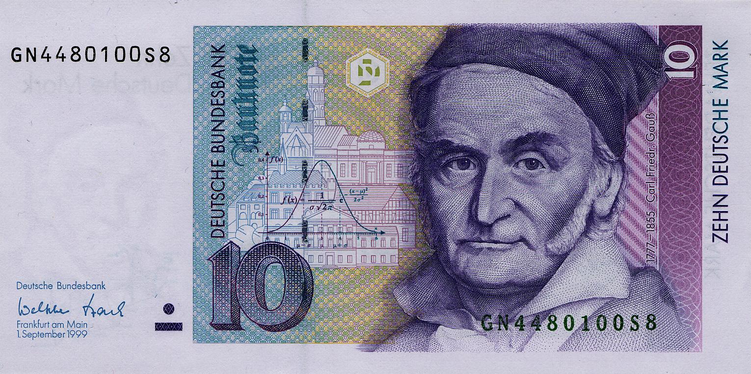
Just for reference, Germany had banknotes for 5, 10, 20, 50, 100, 200, 500, and 1000 (I think the 1000 banknote is a myth; I have never seen it). So, we put Gauss on the 10 banknote. Clearly, he was not as important as some of the others on more valuable banknotes (which were all poets, writers, and one architect, most of whom I have never heard of). There is a reason I don't live in Germany anymore ... I am not a model citizen ...)). Germany, Land der Dichter und Denker ...
Before we start to make our own currency and rank famous CFD people by importance, let's explore the core idea behind the Jacobi method. Let's say we have the following system of equations that we want to solve:
We saw this already in Eq.(12), when we discretised a 1D equation. The Jacobi method also works for dense matrices, i.e. even though we use a sparse matrix here, we can use it just as well for any type of matrix (including those that arise from unstructured grid-based discretisations).
Let's look at the coefficient matrix here first. What we do in the Jacobi method is to split this into its diagonal contribution and its lower and upper triangular matrix. Let's do this first:
Now we use a trick: If you remember back to the beginning of this article, we looked at the main difference between explicit and implicit discretisations. We realised that explicit discretisations lead to a diagonal coefficient matrix, with only a single entry per row. Therefore, we were able to solve for the values in our unknown solution vector (or ) directly. When we looked at implicit systems of equations, we saw that we cannot do this, as we now have more than a single unknown per equation.
Using the matrix decomposition above, we can write this as:
This indicates that all of these coefficients came from terms that are unknown, e.g. from . In the Jacobi method, we now assume that the lower and upper triangular matrices are known, which we can express as:
To make this clear, we can write this as:
If we write the equation in this way, we see that only the diagonal elements are unknown. Then, we can write the equation as:
If we remember back at what we discussed in the beginning of this article, where we looked at the differences between explicit and implicit systems, we saw that explicit equations only have elements on the main diagonal, and so we can solve for them directly. Thus, using this decomposition of the Jacobi matrix into its diagonal and lower/upper triangular matrix, we have essentially just turned our implicit system into an explicit one. If we left things here, we would get a solution, but an explicit one.
This means we loose all favourable properties we gain with implicit systems, most notably that implicit system of equations tend to be unconditionally stable, i.e. regardless of the CFL number, we will get a solution. Explicit systems tend to be very sensitive to the CFL number and easily diverge if we don't set the timestep correctly based on the limitations imposed by an explicit discretisation. This can be shown by the von Neumann stability analysis, something which we have looked at previously.
So, we can't leave Eq.(137) as it is, but we can further refine this idea. Let us write this equation in a different form:
The only thing I have changed here is the superscript letter from to . Since we want to solve for , let us also multiply by so that we isolate on the left-hand side. This gives us:
Instead of advancing the solution from to , i.e. from the previous to the next time level, we take an iterative approach, where we start with . Then, we can use this to compute . Now we can compare, is ? We have to specify how close the solution needs to be in order to be considered approximately equal (which we will do in a second).
If we find that is quite far away from , well, then we set , and we compute Eq.(139) again. We do the same check again, i.e. is ? If it is, we stop and we set , if it isn't, well, we set and evaluate Eq.(139) again, until we have .
This is an iterative procedure, which will force and to have the same value, at least to within some tolerance. If we go back to Eq.(137) now and we set and , then we get:
However, since after we have iterated for a sufficient number of iterations, we can also write this as:
Or, using the equivalence , we have:
Thus, using an iterative approach, we have turned the otherwise explicit system (all variables on the right-hand side are evaluated at time level ) into a fully implicit system. This observation is key, and this will be used in the other methods in this subsection, as well as in matrix-free methods. We always have a system that looks like an explicit system, and we iterate until .
To bring home this point, the following, somewhat pseudo-C++ code shows how the Jacobi method could be implemented:
1 2 3 4 5 6 7 8 9 10 11 12 13 14 15 16 17 18 19 20 | for (int iteration = 0; iteration < maxJacobiIterations; ++iteration) { // update solution xOld = xNew; // calculate new solution for (int i = 0; i < numberOfPoints; ++i) { // contributions from the upper triangular matrix A aE = A(i, i + 1); // contributions from the lower triangular matrix A aW = A(i - 1, i); // calculate new solution xNew(i) = (b(i) - aE * xOld(i) - aW * xOld(i)) / A(i, i); } // check convergence (e.g. eps = 10^-4) if (L2Norm(xNew - xOld) < eps) break; } |
We see here that I have specified a variable called maxJacobiIterations, so we need to tell our Jacobi method the maximum number of iterations we want to use. On line 3, we set the last computed solution xNew to the previous solution xOld, which is the same as in the syntax we used before.
On line 6, we loop over all points in our mesh. If we have an unstructured grid, we typically only have a single loop; if we have a structured grid, we would have as many loops here as we have dimensions. In this case, I am using a 1D structured grid as an example, as we have done before.
On line 8 and 11, we get the coefficients from the upper and lower triangular matrix. Remember, these are coming directly from the coefficient matrix , as , so instead of defining these lower and upper triangular matrices, I am just taking the values from directly. See Eq.(132) and Eq.(133) for the decomposition and where aE and aW are taken from.
On line 14, we compute a new solution for xNew, or . This is the same as Eq.(139). In this equation, we see that we have to multiply the right-hand side by . Here, is just the diagonal of the matrix. To invert the diagonal, we have , where are the diagonal entries for each row . We see that we do this by dividing the right-hand side by A(i, i), while the coefficients aE and aW would be coming from and , respectively.
Once we have updated xNew, i.e. , we go to line 18 and check the norm. If that is smaller than some small value eps, typically in the range of , then we say that xNew and xOld are approximately equal, or . At this point, we break from the Jacobi iteration and continue with the rest of the simulation.
Just to be clear, we have said that the Jacobi method is computing the solution for
Evaluating this system until is equivalent to solving
Both equations will give us a solution to , but the Jacobi algorithm avoids having to invert the matrix at the cost of having to iteratively find a solution for . I just want to stress that even though these equations are different, they solve for the same quantity, so the Jacobi algorithm is just a reformulation of our original system into an easier system that we can solve.
So, we have seen that the Jacobi algorithm can be used to solve for our unknown vector (or in more general terms), and that we use iterations to get to the solution. But at what cost? There is an elegant way we can show mathematically how expensive the Jacobi iteration is. To do that, we have to introduce some new notation.
We saw that we can decompose our coefficient matrix as . We then decomposed this further so that only the diagonal component is multiplied by , while both the lower and upper triangular matrices are multiplied by , and thus, these can be explicitly evaluated and put on the right-hand side of the equation. Let us write this out again. We have:
In this form, we introduce the following notation:
Notice that the minus sign is part of the new matrix . The letters and may seem arbitrary, but these are used in the literature. The otherwise brilliant book by Moukalled et al. does not bother to specify what and is, though they do provide the decomposition of . So, if you go through literature and find and , then you know these are defined as in Eq.(146).
Let us insert this new definition, our linear system of equations becomes:
Now, let's assume we have an exact equation (for example, from an analytic solution which may exist for a simple system). Let us write this as:
Here, states that the solution is exact (analytically known). In the previous two equations, the matrices and are the same. If we subtract the equation with the exact solution from the equation with the approximate solution, then we get:
Since is the exact solution, the differences between or with can be interpreted as an error, since we know the exact value. Let us, therefore, define:
We can insert this definition for the error into Eq.(149) and get:
We can multiply the matrix onto the right-hand side by forming its inverse and have:
We further introduce the shorthand notation and can simplify this equation as:
So what does this equation tell us? Based on some properties of , we can make some judgment on how the error will grow or shrink between iterations. The matrix will have as many rows and columns as there are grid points in our simulation, and so we can compute the error increase/decrease for each row. Though in reality, this isn't really practical. If we have a 1 million cell grid, then we probably don't want to evaluate 1 million errors individially.
Instead, we want some representative value for the matrix , and this is where the spectral radius, which we have discussed before, comes in. As a short reminder, the spectral radius was given in Eq.(59) as:
So, if we apply that to our new matrix , we have:
The spectral radius will look at all eigenvalues and return the largest (absolute) value. We can use this eigenvalue to state something about the convergence speed of the Jacobi method. For example, if the spectral radius of some matrix is found to be , then, according to Eq.(153), the error at the next iteration will be half of that at iteration .
On the other hand, if , then the error at will reduce by a factor of 10 compared to the error at the previous iteration . Thus, the smaller the spectral radius, the faster the error reduction. Remember, the error is a measure between the currently computed solution and the analytically known (correct) solution . So, a reduction in error will bring closer to .
As a result, once we get closer and closer to , the differences between and will become smaller and smaller, and so we reach a converged solution. This means that as long as is smaller than 1, we get convergence, and the closer we are to 0, the faster we converge. However, we can also see that if , the error will increase for each iteration, and we get divergence in our iterative solution procedure. We can write this in a compact form as:
As it turns out, the Jacobi method is simple to implement, perhaps even easy to understand (that is something only you can judge), but this simplicity comes at a cost; it is just awfully slow! (as in, slow factorial ... OK, I stop with the nerdy math jokes ...). And, if we look at the definition for , we see that there isn't much we can do about it:
Since depends entirely on the discretised system and the coefficient matrix that comes out of it, we can't modify this matrix and so the convergence rate of the Jacobi method is fixed and cannot be improved. Thus, if we wanted to improve convergence, we would have to change , and this is what this bloke on the 10 Deutsche Mark banknote did. Let's look at his idea next.
The Gauss-Seidel method
Our story starts in the summer of 1821, in the Kingdom of Hannover. It was created along 38 other, sovereign, states within the German Confederation, in the wake of the collapse of the Holy Roman Empire (which existed for pretty much 1000 years, covering what now is known as Germany), all thanks to the Napoleonic Wars, which were fought by the French between 1803-1815. A small Frenchman was able to bring an Empire to its knees in a decade that existed for a millennium. I believe this is the reason we all love the French in Europe, right?
In 1819, a conference was held in Karlsbad by the German Confederation, and the Carlsbad Decrees were signed. This was aimed at cracking down on nationalism and introducing stronger censorship to suppress liberal ideas. Universities came under scrutiny, and liberal professors were removed. Amids all of this, the government of the Kingdom of Hannover, which was geographically in what is now Germany but ruled by George IV (the King of the United Kingdom, makes sense), approached Gauss with a Task: They wanted to know how big their Kingdom was.
I'd love to think this was purely done for flexing, with George IV sending Twitter messages to his King friends asking How big is yours? (Kingdom, what did yo think?), but, with state lines shifting, the government needed to know what belonged to their Kingdom so they could tax people within the Kingdom correctly. Certainly, the military also had an interest in knowing where its borders were.
So, we had the Carlsbad Decrees, specifically targeting university professors (which Gauss was at that time), which, in many ways, was Germany's first attempt to establish a North Korean like regime (what is the difference between a dictator and a king with strong censorship?). We tried again, some 100 years later, with East Germany, proper communism and all of that Jazz, but we failed for a second time to establish a North Korea in the heart of Berlin.
As they say: Third time's a charm, so who knows, perhaps there is a third, successful attempt in the year 2130 in whih Germany will have become a worthy successor of the North Korean Empire (at which point, we will be driving North Korean branded Hyundai and Kia cars). I really should stop now, I don't want to become the next Jonny Somali ...
So, the scene is set, and Gauss began to measure the Kingdom. Similar efforts were completed earlier when the Kingdom of Denmark was measured, and Gauss received help from them. At the same time, other states wanted to know their kingdom's size and boundaries to properly tax their citizens. But the way Gauss did it was special. Gauss didn't just measure the Kingdom of Hannover; he invented a whole new scientific discipline.
By the time Gauss started his measurement, he was already famous like Einstein (of course, people would not compare him to Einstein back then; he wasn't born yet). The way he went about his measurements was to measure a triangle on a flat surface and use that as his baseline. Knowing the exact properties of one triangle laid out on a flat surface (length of each side and angles), Gauss could then determine the properties of other triangles of much larger size.
So far, we have only used trigonometry, i.e. Gauss could stand on a tall building, or tower, and measure the angle between two points he could observe in the distance. He would repeat the same measurement on the other points, and then he could determine the area of each triangle. But there is one problem. Let's look at his measurement in the following sketch:
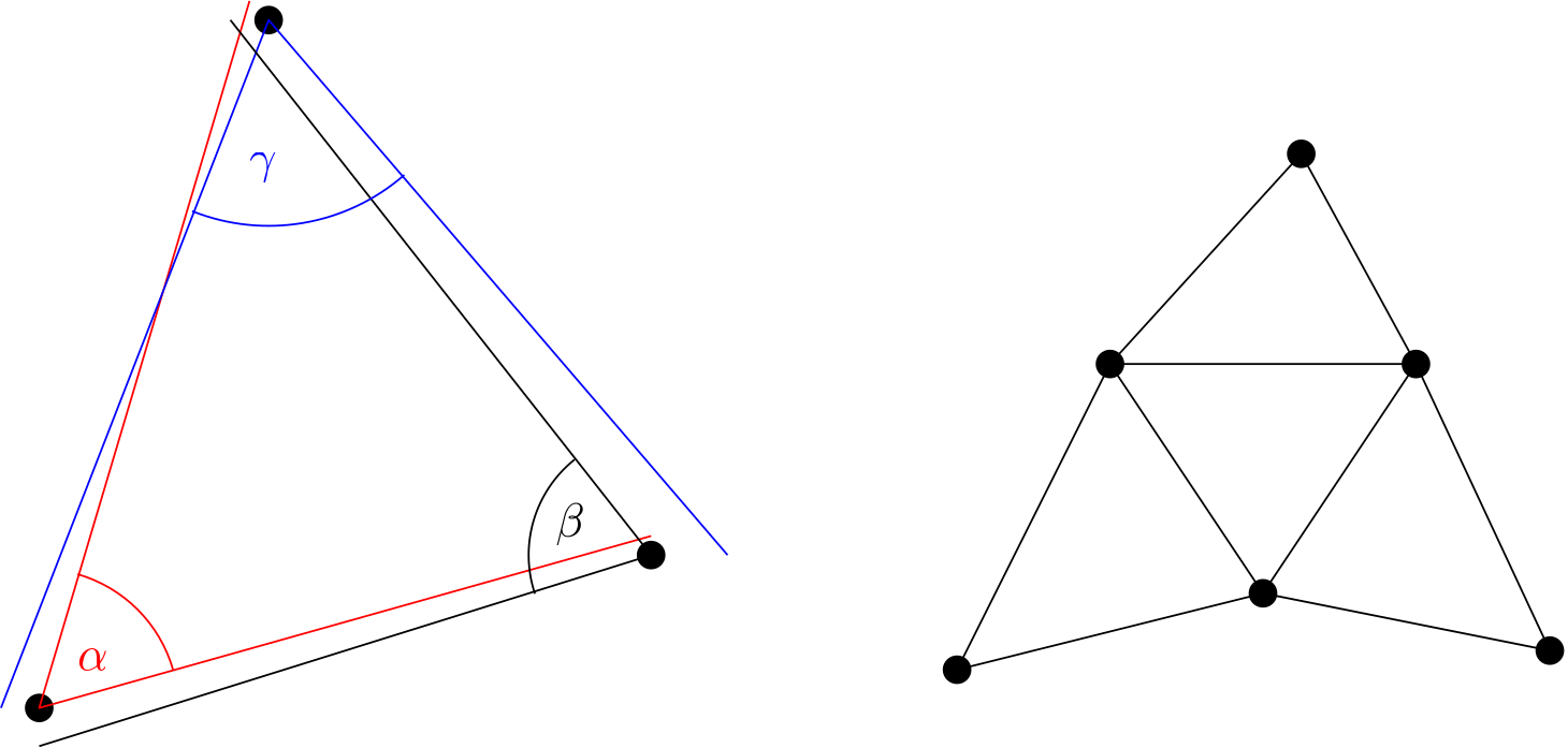
On the left, we see three points. Let's say we want to compute the area of the triangle that is spanned by these three points. If we follow Gauss, then we could look for three tall buildings, climb on top of each of them, and then measure the angle between each. Even today, we would make a small error in determining the angle between these three points; imagine how Gauss must have felt doing all by hand.
As we can see from the sketch, we will make a small error in determining the angle. In fact, we can get an idea for how accurate our measurement is by adding up all angle, i.e. . Within a triangle, we know that all of that should add up to , and it is unlikely that we get this value from our hand measurements.
Now, Gauss did not just span one triangle over the entire Kingdom of Hannover, but there were several triangles, leading to a network of triangles, as shown on the right. Here, all the angles between edges that meet at vertices will have a small error. We could leave it at that and accept that we will get a small error in our calculation, but Gauss wasn't happy with that.
Instead, he knew that all angles in a triangle should add up to and he used that to his advantage. But, since edges between triangles are shared, making changes to one triangle (making changes to one of the angles) will influence neighbouring triangles as well. So, the problem becomes one of minimising the error globally for all triangles when adjusting the angles.
Thankfully, while the Napoleonic Wars were in full swing, Gauss was busy publishing a method that we know as the least square problem nowadays. He could use the least squares problem here as well to minimise measurement inaccuracies. We looked at the least squares problem already, when we looked at Eigen and how to solve it with code. You can have a quick look at it, but you won't need it to follow the rest of the discussion.
However, what I did show in the article is that a least squares problem can be formulated as:
Well, that is the starting point, but since the matrix may not be a square matrix (i.e. the number of rows and column may not be the same), we have to make it square first. We do that by multiplying both sides by the transpose of and have:
What we can see is that the solution to the least square problem can be formulated in a linear system of equation form . And so, Gauss needed a way to solve this equation. Even for him, Gaussian elimination was too expensive based on all of the triangles he had, and so he needed a cheaper solution. Krylov wasn't around, but Gauss, in a typical Gauss fashion, simply invented a new method to help him solve his problems, which he never published.
However, he used this method to correct his triangle network so to get a more accurate reading on the area of the Kingdom of Hannover. In fact, remember the banknote I showed you earlier? Well, if we turn it around, this is what we see:
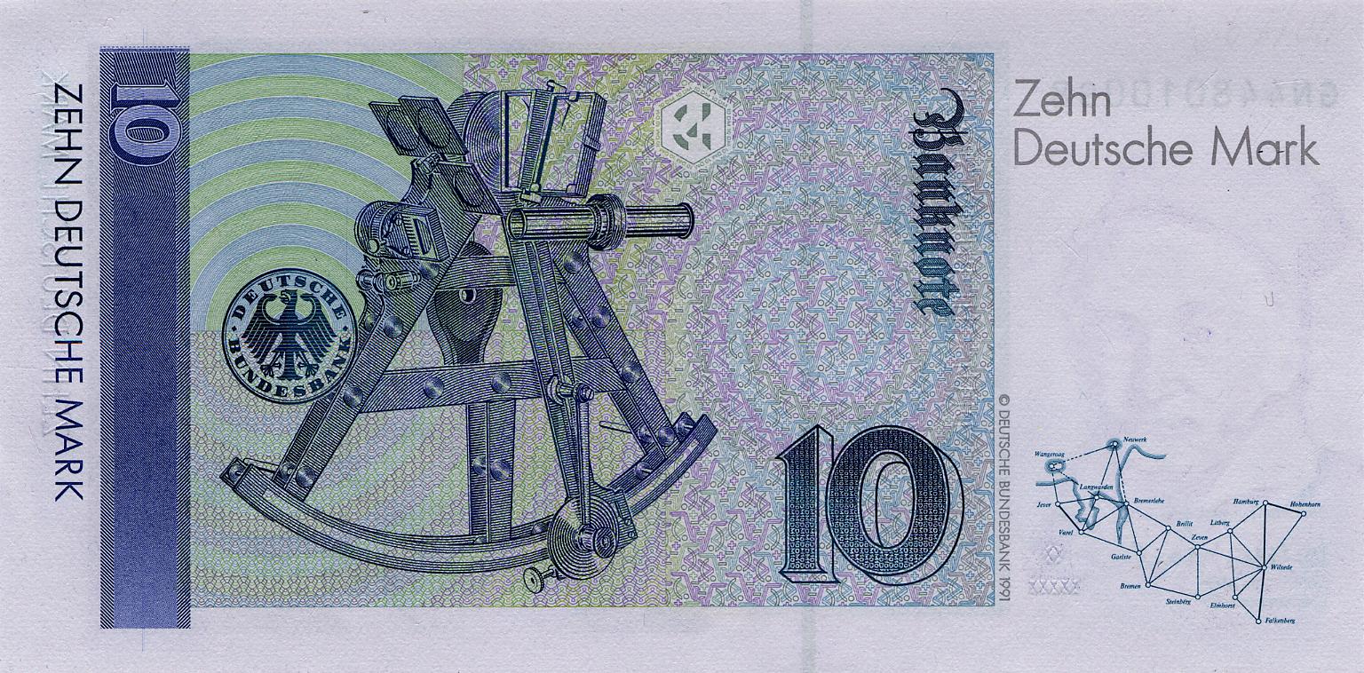
The bottom right corner shows Gauss' triangular network of the Kingdom of Hannover. I only found out now. The Deutsche Mark was replaced by the Euro when I was 13 years old, so I suppose I did not have the strongest of interests in Gauss' work back then, so I never noticed. I did, however, read the book Die Vermessung der Welt, which I thought was quite good back then; still, I had no idea about Gauss' triangulation (and the book literally deals with Gauss' attempt to measure the Kingdom).
So, what was that method I referred to? The method is known as the Gauss-Seidel method nowadays, and you will find it in general purpose CFD solvers. Gauss had no interest in publishing this method; he didn't see it as important. Some 50 years later, Seidel decided that perhaps some people may be interested in this method, and so he published it. In a true academic fashion, one person does all the work, and then the vultures come in, add their name to a paper, and get famous alongside. Academia isn't broken ...
In any case, let us have a look at the Gauss-Seidel method then. We can do that by looking at the starting point of the Jacobi method. We said that we can decompose a coefficient matrix into its main diagonal, as well as its lower and upper triangle. We can use this decomposition to solve the linear system of equations as:
This was Jacobi. For the Gauss-Seidel algorithm, we make one small change:
Yes, that's it. This is the Gauss-Seidel algorithm in full display. I could stop here and move on, but it is worthwhile exploring why this method is better than the Jacobi method. First of all, we can look at the spectral radius. We said that we can decompose the coefficient matrix into an and matrix, where collects all matrices that multiply , while collects all matrices that multiply .
Before we do that, we have to put the known vector on the right-hand side. Then, we can insert our definition for and . This gives us:
Solving this for , we get:
In the previous section on the Jacobi method, we saw that subtracting an exact equation from this equation produced an error equation of the form:
If we look at the equation, we have:
If we compare that with the matrix we obtained from the Jacobi method, we had:
I am using the subscript and to indicate that these are coming from the Gauss-Seidel and Jacobi method, respectively. So, while we can't really see if one of them is better than the other, we can say, however, that . And, therefore, we can also say that:
Well, but we still don't know which of these will give us a lower spectral radius. But we can build up a reasonable intuition by bringing Eq.(160) and Eq.(161) into coefficient form. To get the coefficient form, we simply write out the explicit coefficients we use here. For example, the diagonal matrix contains only elements on the main diagonal. If I wanted to index my matrix , and only get elements on the diagonal, well, I need to index rows and columns with the same index.
If my rows are indexed with the index and my columns are indexed with the index , then, to get an element on the diagonal, must be equal to , i.e. . We could write this as , but that is very abstract, and we cannot really insert that into an equation. We can shortcut this and simply write . So, whatever row we are in, we are going to select the same column and are guaranteed to get the element on the diagonal.
So, we can start to transform Eq.(160) and Eq.(161) by removing the diagonal term and get:
Now we need to think about the lower and upper matrix. To do that let's look back at Eq.(133), where we had:
Let's say I am in the third row (). If I wanted to get the diagonal entry, we said we have . And if I wanted to get all elements in the lower triangular matrix? Well, we see that we have one entry to the left of . That is, in the lower triangular matrix, we have . In index form, we could write this as .
Since the lower triangular matrix is, well, a matrix, we have to evaluate the matrix vector product. In Eq.(161), for example, we have to evaluate . If we are in row three in our example matrix above, then we can write this out explicitly as:
This is now one example, but we want to generalise this. First, we notice that the column index of the matrix is the same as the index of our unknown vector . Next, we are in row three, so . We also notice that we have a summation of two terms, so we want to express that with a summation. Let's give this a try. The above equation can be generalised as:
We start the summation in the first column, hence the summation operation starts at . We are in the third row, and the lower triangular matrix does not include the main diagonal, so the summation has to stop before the diagonal. The diagonal is at , so the summation needs to stop at (and we saw that we only had two terms in our summation before, this part checks out).
Then, are simply the coefficients in the lower triangular matrix, while are the components in our unknown solution vector . So, inserting this into Eq.(168), we have:
What about the matrix ? Well, this is just the upper triangular matrix, so we have to do something very similar to the lower triangular matrix. Instead of summing from to , which covers all entries in the lower triangular matrix up until the diagonal, we have to do the sum from to , where is the number of rows and columns in our coefficient matrix . If we do that, we can write, for example:
The summation we have to evaluate hasn't changed; only the start and end of the summation. So, we can insert that into Eq.(172) and obtain:
The only vector left in this expression is the right-hand side vector and the unknown vector multiplying the diagonal coefficient. Since we go through this equation row by row, i.e. we go through each row in our matrix with index , we have to replace both and by their -th component. Thus, we replace these vectors with and , respectively, and we get:
Remember, the first equation is our Jacobi method, the second equation is our Gauss-Seidel equation. We can solve both of these now for and see what the resulting update equation is. I will split both equations now into their own equation so we can look at them separately. For the Jacobi method, we get:
For the Gauss-Seidel method, we get:
Hang on, for the Gauss-Seidel method, we now have on the left-hand side and on the right-hand side. Didn't we just say that we wanted to collect all unknowns on the left-hand side? Yes, we did that. But why is on the right-hand side? Well, even though it is, at some point, unknown, once we evaluate , it is already known.
Remember, multiplies only the lower triangular matrix, which goes from to . This, when we evaluate , say, for example, we are in the third row and have , then we want to compute . But, the lower triangular matrix goes only up until . So, the lower matrix coefficients are multiplied by and .
If we iterate over all rows in the matrix, typically starting at the beginning, i.e. row 1, and looping to the last row, then, at the time we evaluate , we have already computed and in a previous iteration. Thus, once we compute , we have already computed and . Since we only need these previously computed values in our lower triangular coefficient matrix, we can write this on our right-hand side and assume these values are know.
This is the reason why the Gauss-Seidel method is faster, by approximately a factor of two, compared to the Jacobi method, because it uses the updated solution immediately in each iteration. The best part about the Gauss-Seidel method is that once you have implemented the Jacobi method, getting the Gauss-Seidel method implemented is straightforward.
Let's modify the pseudo C++ code we have seen before for the Jacobi method. To modify it and make it the Gauss-Seidel method, this is what we have to do:
1 2 3 4 5 6 7 8 9 10 11 12 13 14 15 16 17 18 19 20 | for (int iteration = 0; iteration < maxJacobiIterations; ++iteration) { // update solution xOld = xNew; // calculate new solution for (int i = 0; i < numberOfPoints; ++i) { // contributions from the upper triangular matrix A aE = A(i, i + 1); // contributions from the lower triangular matrix A aW = A(i - 1, i); // calculate new solution xNew(i) = (b(i) - aE * xNew(i) - aW * xNew(i)) / A(i, i); } // check convergence (e.g. eps = 10^-4) if (L2Norm(xNew - xOld) < eps) break; } |
Did you spot the difference? The only change we have to do is on line 14, where we have replaced all xOld arrays by xNew arrays. Essentially, we are reading and writing here to the same array and use an updated solution here if already available. If not, well, then we simply take the solution that we had in the array from the previous iteration (or initial condition).
I do use both xNew and xOld here, but I only keep xOld around so that I can compute the difference between two iterations to check if the solution has converged. However, if we don't need to check for convergence, and we know we are only ever going to use it for a few iterations (for example, during a multigrid cycle), then we can remove the convergence checking and simplify the Gauss-Seidel method to:
1 2 3 4 5 6 7 8 9 10 11 12 13 | for (int iteration = 0; iteration < maxJacobiIterations; ++iteration) { // calculate new solution for (int i = 0; i < numberOfPoints; ++i) { // contributions from the upper triangular matrix A aE = A(i, i + 1); // contributions from the lower triangular matrix A aW = A(i - 1, i); // calculate new solution x(i) = (b(i) - aE * x(i) - aW * x(i)) / A(i, i); } } |
In this case, we have only a single x array, which we constantly write to and read from at the same time. We have reduced the storage requirements now by a factor of two (we only store one array, not two arrays), and we have gained convergence acceleration by a factor of about two. Not bad for such a small change!
In the Gauss-Seidel algorithm, for example, in the pseudo code given above, we always looped from the first row of the coefficient matrix to the last row, or, in terms of our loop, we started at and went to the numberOfPoints. This is known as the forward Gauss Seidel. Now, here is a tough nut for you to crack. Can you imagine what the backward Gauss Seidel method is doing?
If you guessed going from the back (last row) to the front (first row), wow, you are on your way to a Nobel Prize! (I mean, Gauss set xOld=xNew and called this a new method, Seidel didn't do anything besides publish this, and we remember his name for it. If this is the bar for claiming academic fame, a Nobel Prize can't be that difficult to obtain, I reckon...)
Ok, we know what the forward and backward Gauss-Seidel method (forward and backward looping), but riddle me this: What is the symmetric Gauss-Seidel method? Well, this is a good application of Occam's razor, which essentially states that the most logical solution is the simplest one. This is one example where we are allowed to use business mathematics:
So, the symmetric Gauss-Seidel method does a forward sweep first, followed by a backward sweep. Why is this a good idea? If we are only doing a forward or backward sweep, information will always propagate in one direction. However, if we do a symmetric sweep, information can propagate in different directions. To make this clear, take a look at the discretisation of the Laplacian operator in one dimension, for example:
Here, we can see that if we used a forward Gauss-Seidel method, for example, we would always update the solution such that would already be known (always, as this is coming from the lower triangular matrix) when we update , so the solution for is always lagging behind. This asymmetry can then introduce a directional dependence which may slow down convergence.
The cure is to use a symmetric Gauss-Seidel method in this case, which will update and in an alternating fashion, aiding to preserve the character of the Laplacian operator (diffusion in each direction in equal parts, rather than stronger diffusion in one direction). These types of operators lead to symmetric matrices.
We can see from Eq.(179) that the contributions to the lower and upper triangular matrices and are going to be the same, so the coefficient matrix , which consists of the diagonal, upper, and lower triangular matrix, i.e. , is going to be a symmetric matrix. For these types of matrices, the symmetric Gauss-Seidel method has computational advantages (it may converge faster) over the pure forward or backward Gauss-Seidel method.
In pseudo C++ code, we can write this as:
1 2 3 4 5 6 7 8 9 10 11 12 13 14 15 16 17 18 19 20 21 22 23 24 25 | for (int iteration = 0; iteration < maxJacobiIterations; ++iteration) { // forward sweep for (int i = 0; i < numberOfPoints; ++i) { // contributions from the upper triangular matrix A aE = A(i, i + 1); // contributions from the lower triangular matrix A aW = A(i - 1, i); // calculate new solution x(i) = (b(i) - aE * x(i) - aW * x(i)) / A(i, i); } // backward sweep for (int i = numberOfPoints - 1; i >= 0; --i) { // contributions from the upper triangular matrix A aE = A(i, i + 1); // contributions from the lower triangular matrix A aW = A(i - 1, i); // calculate new solution x(i) = (b(i) - aE * x(i) - aW * x(i)) / A(i, i); } } |
Finally, you may ask, what is business mathematics? It's when we add words together and pretend it's maths. Next time you see someone use business math, you have my permission to write an integral in front of each word and integrate the constant 1 from 0 to 1 (which is, well, 1). We haven't changed anything, the equation is still correct, but business math people won't realise. So much much for business math ...
Successive Over-relaxation (SOR)
Let's talk about under-relaxation for a moment. When we solve linear partial differential equations, we can simply form a discretised version of them and then compute an updated solution. Job done! But with non-linear partial differential equations, small inaccuracies can quickly multiply and lead to divergence in our simulations.
If we look at the SIMPLE method, which was introduced to solve incompressible flows and, in my view, is a blatant rip-off and plagiarised (and somehow inferior) method based on Chorin's exact pressure projection method, Patankar and Spalding butchered Chorin's pressure projection method so badly that they would no longer give us an accurate prediction of the flow.
Some may say this was required to take away some of that non-linearity so as to stabilise the non-linear partial differential equations and, as a result, the flow field as well. However, I'd argue that we could have done the same with Chorin's exact pressure projection method but well, I don't teach at Imperial College so obviously my opinions aren't as valuable.
I mean, if you cut yourself in the finger, if you wanted to stop the bleeding, I'd argue applying a bandaid is a sensible solution. However, if we apply the same logic as the SIMPLE algorithm here, we would have to chop off our hand. Sure, it will stop the bleeding on our finger, but we have just created a dumpster fire of other issues elsewhere.
So, the SIMPLE algorithm by itself doesn't work. We linearise an otherwise non-linear partial differential equation, and we even get rid of parts of the non-linear term, just to make our life easier (or simpler?). But then, we realise, we probably can do better, and we bring back these non-linear terms we have dropped, and this allows us to introduce a new method, called the SIMPLEC method, where the C stands for consistent. In reality, the SIMPLEC method only brings the SIMPLE method closer to Chorin's exact projection method.
In any case, let's focus on the SIMPLE algorithm. It has so many simplification that we are only getting an approximate prediction of the flow (once we get convergence, we will recover a sensible flow field again, as it still retains Chorin's pressure projection core ideas). This means that if we were to update our solution with the SIMPLE algorithm and then continue to update our solution with these new updates fields, we would eventually get divergence in our simulations.
So, we introduce a fix, called under-relaxation. What we do here is to only update our new solution by a fraction (somewhere between 0 and 1, or 0% and 100%). We write this as:
Here, is known as an under-relaxation parameter, and it takes values between . While Chorin's pressure projection method can operate with pretty confidently (eventually we may need to use some form of under-relaxation if we start to use turbulence models, which themselves are not exact), the SIMPLE algorithm requires heavy under-relaxation. Values of and are common for the velocity field and pressure field, respectively.
If we insert , for example, into Eq.(180), we see that we are now taking only 0.7 of the newly computed solution, and we add from the previously computed solution, i.e. the solution at time level . So, we can see under-relaxation also as a weighted sum, or linear blend between two quantities.
This under-relaxation stabilises the SIMPLE algorithm sufficiently so that solutions can be obtained again. As the name under-relaxation suggests, values of are in the range of , as already highlighted. But, we can also introduce over-relaxation, where we require . If we tried to do that, we would get divergence, and so, over-relaxation isn't something we commonly use in CFD. Except for one case: The Gauss-Seidel method.
Yes, this is now, what, the 5th section or so where we talk about Gauss again? I told you, we can't do linear algebra without Gauss, just like we can't have the UK without mildly offensive border security guards at Heathrow Airport. They love welcoming foreigners (with fully settled status) into their little Kingdom ... It is just part of the deal (and I shall avoid heathrow airport for a while). Is now the right time to talk about the time I smuggled German sausages into Korea? Perhaps a story for another time ...
So, let us apply the same idea of under-relaxation to the Gauss-Seidel method. I will then show you how this under-relaxation can actually lead to stable results with over-relaxation. Happy days!
Let's look at the Gauss-Seidel algorithm again, which was given in Eq.(177). For convenience, I have repeated it below:
The right-hand side is now updating the left-hand side fully, but we want to write the right-hand side in the form of Eq.(180). We can do this by introducing the relaxation parameter (as it is usually used in the literature) and write:
Or, rearranging terms, we can also write:
This is perhaps more commonly used in the literature, but both are the same equation. So, we multiply the term that updates by , and then, we have to introduce and multiply that by to get a weighted average between the solution at and . The question is, what values can we choose for so that the solution is still stable?
Well, we have already established that for the simulation to converge, we require that the spectral radius of the matrix is less than 1. As long as that is given, we will get convergence. The spectral radius, as defined in Eq.(59), says that it is the largest (absolute) eigenvalue of a matrix. So, we need to do 2 things: First, we need to derive the matrix which contains , and then we need to compute its eigenvalues, and solve those for .
Let's start by deriving the iteration matrix . From Eq.(161), we saw that the Gauss-Seidel method is given as:
We bring the contributions of to the right-hand side and get:
Here, I have started to use the notation to show that this unknown solution vector is obtained from the Gauss-Seidel method. Now, let's remind ourselves of the SOR definition. We said that this is coming from Eq.(180), and so we can write this, using the SOR factor , instead of , as:
Here, is the solution we obtain from the Gauss-Seidel algorithm, i.e. Eq.(185). Let's isolate that on the left-hand side:
We divide this now by , which provides us with the final form:
We can insert this definition now back into Eq.(185) and get:
We multiply this equation by and get:
Let us now expand the left-hand side. We have:
Let's further expand the left-hand side:
Let me rewrite this equation as:
Let's look at Eq.(186) for a moment. If we multiply this equation on each side with , then we get:
Solving for , we get:
Noting that , since we already inserted this into our Gauss-Seidel algorithm, we can rewrite Eq.(193) as:
Now, you may be saying, we can do the same for the first two terms involving , right? OK, let's do that and see what happens. We can write the SOR definition, now multiplied by , as:
We insert that definition into Eq.(196), noting again that , and we get:
Now we notice that each term contains , so we can divide each term by it:
Finally, we can simplify the left-hand side to:
We just obtained Eq.(185) again, which was the starting point for our derivation. So, surely, this is not what we want. Instead, let's go back to Eq.(196) and leave the terms involving as they are on the left-hand side. The next step in our derivation requires us to bring to the right-hand side. This gives us:
Now we introduce a little trick to make the signs the same. The following definition holds:
If you don't believe me, insert any value for , and you will see this is correct. We can use this to rewrite our equation as:
The second and third terms both contain a on the right-hand side, let's factor that out and write:
Now, onto the left-hand side, we can rewrite this in a more compact form as:
Comparing this with the original Gauss-Seidel method without any SOR treatment, we had:
We see that the left-hand side remains the same, apart from the relaxation factor . We also see that the right-hand side is slightly modified, but more crucially, we see that dividing this entire equation by will not get rid of it. This is, perhaps, the best intuitive approach I can show you that this form is correct, and not the one we saw before, where cancels from the equation.
We can now, again, define an exact solution and form the same SOR system:
If we subtract Eq.(207) from Eq.(205), we get:
Introducing the error notation again where and , we get:
Solving for the error , we get:
Thus, we can define our matrix as:
From our spectral radius definition, we know that this converges for . However, we also know that the spectral radius is nothing more than the largest (absolute) eigenvalue of , i.e. . So, we need the eigenvalues of . The eigenvalues are obtained by evaluating and setting this to zero, i.e.:
Let's apply that to an example for the matrix:
The eigenvalues can be computed as:
Here, I have defined the constants , , and . We can use the abc formula to solve this quadratic equation as:
Since is set equal to zero when evaluating the eigenvalues, we also have as we saw above. We can rewrite this equation, knowing the eigenvalues now, as:
If we insert either 1 or 3 into the equation, i.e. our eigenvalues, then the right-hand side will be equal to zero. We can generalise this as:
More generally, we can write:
Remember what our goal is. We have the matrix given, and we want to relate that to our eigenvalues . Specifically, we want to know which is the largest eigenvalue, so that we can evaluate the spectral radius. In the equation given above, is just a variable, whereas are our eigenvalues. Therefore, we can set and get:
Here, is the number of rows and columns of , i.e. we have as many eigenvalues as there are rows in the matrix. How does this help us? Well, we said that in order to have convergence, we need the spectral radius, that is, the largest eigenvalue, to be smaller than 1. However, Eq.(219) gives the product of all eigenvalues; we can't easily extract the largest eigenvalue from it.
Here is the trick: We say that in order for the spectral radius to be larger than 1, we need to have at least one eigenvalue that is larger than 1. If all eigenvalues are less than 1, then their product will also be less than one. However, if one eigenvalue is larger than 1, it is possible for the product to be larger than 1 as well.
Now, I should state here that this is only one condition, for it is possible to have eigenvalues that are larger than 1, but the products of all eigenvalues is less than one. If I have and , then the product is . The product is less than one, but the largest individual eigenvalue is larger than one.
So, while Eq.(219) doesn't say anything about the largest eigenvalues, we can still use it. That is, if the product of all eigenvalues is larger than 1, that tells us that at least one eigenvalue is larger than one as well, as already established. It turns out that, even though this is a weaker requirement than checking the absolute largest eigenvalue, it still works in practice very well.
So, what we do is to say that in order for the SOR Gauss-Seidel method to work and converge, we have the requirement:
Notice that it is the absolute value of the eigenvalues now, i.e. the eigenvalues can be negative. This comes from the definition of the spectral radius, i.e. Eq.(59).
OK, so let's evaluate this expression. First, let us remind ourselves what the matrix was, which I have repeated below for convenience:
We want to take the determinant of this now. There are a few rules for determinants that we can apply here. The following properties hold:
Using these properties, we can write the determinant of as:
We now need to evaluate these determinants separately. For a 3-by-3 matrix, we can use the rule of Sarrus, where we copy the first two columns to the right, and develop our determinant as shown in the figure below on the left:
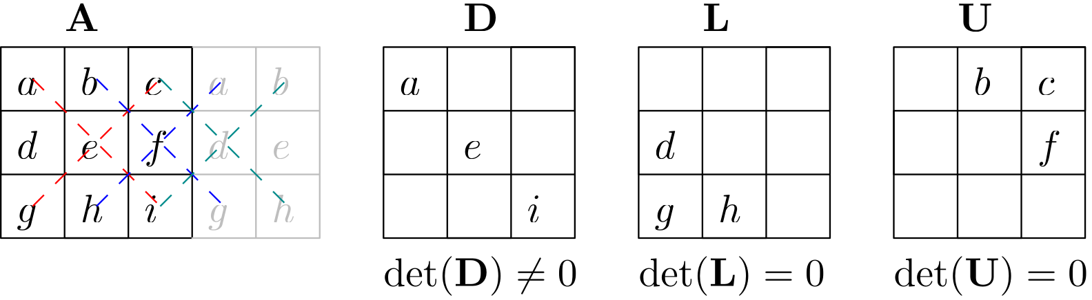
Here, we have that the determinant for the matrix is:
We can see that the determinant essentially adds and subtracts products of diagonals and off-diagonals. Let's apply this to the diagonal matrix . This matrix has, by definition, the main diagonal of matrix . As long as the values on the diagonal are not zero (which they are not for CFD applications), then we will have a non-zero determinant. This is also shown in the figure above.
In the same figure, I have also given the determinants for the lower and upper triangular matrix and . I have removed entries here which would be zero. We can see that if we apply the rule of Sarrus to either or , there will always be at least one term that will be zero. As a result, both and will have a determinant that is zero.
We can use that now in Eq.(223). Let us look at the determinants for both the numerator and denominator separately. For the numerator, we have:
If we look now at diagonal entries, only has one full diagonal with non-zero entries. Therefore, we can write the determinant expression as:
Here, we are summing the individual contributions in , i.e. with the expression given inside the brackets, i.e. , which gives us the only non-zero diagonal contribution and thus determinant. We can remove the summation and write this in matrix form as:
Since the determinant of is just the sum of all of its diagonal entries (as all other off-diagonals will be zero), we can replace the summation here by the determinant. The only thing we have to change here is that the expression given in parentheses is now raised to the power of , as we have to multiply it times with the coefficients in .
OK, return to Eq.(223), the denominator can be evaluated as:
Here, we use the same argument again that only will contribute to non-zero products in the development of the diagonal, whereas all terms of the lower triangular matrix will have zeros in their product, and thus it plays no further role in the development of the determinant.
If we insert now the simplified expressions for the numerator and denominator back into Eq.(223), we get:
We can use this expression now and insert that back into Eq.(220). This gives us:
The determinant can be positive or negative, but since it is used here to compute eigenvalues (for which we have to take the absolute value), we are now using the absolute value of . We need to solve this expression now for . The first step is to take the -root () of both side. This gives us:
Now we can check for which ranges of the inequality holds. We can that if , the expression becomes:
Thus, is the lower limit at which point convergence is no longer given (it is also the trivial answer as an under-relaxation factor of zero just means we are not updating the solution at all!). So, we need to set to get stable convergence. If we set , then we get:
Again, a value of is just over the limit and we will get neither convergence nor divergence. So, the upper limit of is two, and we can write this in a compact form as:
This is the requirement for , and, unlike under-relaxation factors, in the SOR method (which literally stands for successive over-relaxation), we are able to over-relax the Gauss-Seidel method and thus accelerate convergence. This is one rare instance in CFD where you get quite a lot of return on essentially a zero investment (all we have to do is multiply our Gauss-Seidel algorithm by some s).
Thus, in the extreme case of , we can get a convergence acceleration of 4 compared to the Jacobi method. Not bad for simply setting xOld=xNew and multiplying by one factor.
Damn, I just realised, I'll be flying out of Heathrow in a few weeks again. Oh boy ...
Lower-Upper Symmetric Gauss-Seidel (LU-SGS)
If you thought we would be done with Gauss, I'm sorry to disappoint you; he is here to stay, and we need to talk about yet another method. It is a bit of a stretch to call it another method. The lower-upper, symmetric Gauss-Seidel, or LU-SGS method, is nothing but the pure symmetric Gauss-Seidel method. It seems perhaps more of a footnote lost to history that some people prefer to use the terminology LU-SGS, while others simply stick with the symmetric Gauss-Seidel terminology.
To the best of my knowledge, LU-SGS is what people use in the compressible flow community, while others (especially incompressible flow developers) use the symemtric Gauss-Seidel terminology. Again, both methods are algebraically identical; they just have a different name.
However, despite being algebraically different, the way the methods are derived is slightly different. For the Gauss-Seidel method, we simply set to if the solution was already updated inside the loop from to . That's not much of a derivation, granted.
In the LU-SGS method, the starting point is, in a very anticlimactic fashion, the LU decomposition. So, let us look at the derivation and see for ourselves that the LU-SGS method does indeed simply produce the symmetric Gauss-Seidel method.
The starting point for the LU decomposition was to split the matrix into a lower and upper triangular matrix, such that if we multiplied both, we would get the original matrix back. We can express this as:
We saw in the section on the LU decomposition that forming and costs just as much as doing the Gauss elimination, which is prohibitively slow. For that reason, we don't want to find an exact LU decomposition, but rather an approximate LU decomposition. Ideally, we only want to use information we already have as well, so we don't need to compute extra bits and pieces.
Thus far in our discussion, we have often decomposed the coefficient matrix as:
Since we have all the matrices available, our goal is to use these to find an approximate LU decomposition. A first idea may be to use:
However, if we carry out the multiplication between the brackets, then we obtain the following:
We now get a term , as well as a combined . Why is this a problem? Remember, the goal is to express through already known matrices, and we said that when we decompose the coefficient matrix , we did so by writing . So, we are looking for approximation to that result in .
Since by itself gives us additional terms, such as , we need to modify this term slightly. Now think about it yourself. If you have the number , and you want to get rid of the power, you could take the square root, yes, but that wouldn't work on matrices. But, we can write , and so, if we now want to get rid of the power of two, we could also write or .
We can take the inverse of a matrix, and so, if we want to get rid of power in the , because we are trying to obtain a form of , then we simply multiply by , because . Makes sense? So, let's do that. We multiply both parenthesis by and we get:
Let's carry out the multiplication for the first term with . We get:
If our diagonal contains entries like , then its inverse () will contain entries like . Remember, if you only have the diagonal in a matrix (and, after all, is still a matrix, but the letter D indicates that it only has entries on the diagonal), we can find the inverse of that matrix with ease by inverting the diagonal.
Thus, if we compute now , then we will evaluate products like , and therefore, , where is the identity matrix.
We can now multiply the term obtained from Eq.(240) with the second term in Eq.(239) and get:
Acknowledging that any matrix multiplied by the identity matrix will give back the original matrix. Furthermore, we see that we have again, which is the identity matrix. Since the identity matrix does not modify a matrix if we multiply by it, we can drop it and obtain:
We can write this as:
We have almost reached our goal, that is, to find an approximation to that results in a decomposition of the form , but we have obtained an additional term, which we now need to get rid of. How do we do that?
Well, we could turn to our friends at Heathrow airport and ask a border patrol agent what they would do, but their answer probably would be just deport it. Now, I have checked, but there doesn't seem to be a deportation operator we could use here, and so we have to use a bit of logic instead. First, we write the term on the right-hand side so that the matrix is again isolated on the left. We have:
Now comes our logic, or trick. We say: and therefore we drop it altogether. Why can we do this? Well, we can use the so-called boundness property, which was formulated in 1958 by Scarborough. To do that, we need to write in coefficient form first. For that, we make the following substitutions:
Then, we can write:
Scarborough says that the following inequality must hold:
Compare the two states. While the boundness property adds the summations in the numerator, we multiply them in Eq.(246). The boundness property is a necessary condition for convergence, and, indeed, the diagonal typically contains the largest elements in the entire coefficient matrix. Thus, if we look at , we see that we scale both and by the inverse of , and must be greater than and combined.
Why is this typically the case? The timestep only appears in the matrix, not in the and matrices, and this typically results in being at least an order of magnitude greater. For example, if we had the following PDE:
Then we could discretise it with a simple first-order forward in time and second-order central scheme in space (using the finite difference method) as:
We can now write this in terms of the factors of and get:
Now we collect terms at on the left-hand side and terms of on the right-hand side:
We can now combine the two terms at :
Terms at will go into our diagonal matrix , while terms at and will go into and , respectively. Thus, we could write this as:
Therefore, we have:
Now we can do some order of magnitude estimates. Let's start with . Looking at some values for the thermal diffusivity, we have values between . For example, we have for air and for water (measured in ).
From the CFL condition for purely diffusion flows, we have:
Let's rewrite this as:
If we say that ranges between , let's pick an average . Let's insert this into our equation:
We can now assume that our CFL number is typically of the order of 1 to 100. Then, we can write:
In other words, it is fair to say that , and this is true for convection-driven flows as well (in this case, we only looked at thermal diffusion). Let's pick a moderate CFL number of 10. Let's also pick an arbitrary spacing of . Then, we can compute the timestep to be:
Thus, we have while we have , and indeed, we have . Let's go back to Eq.(254) and insert these values:
Let's go back to our original statement that . We can now write out our order of magnitude estimates for this particular case:
We can see that there is about an order of magnitude difference, and this difference will only get larger as we add convection and thre-dimensionality to the picture. Thus, if is OK to drop .
Therefore, return to Eq.(244), which was given as:
It is reasonable to write it as:
This might seem that we haven't really gained anything, but remember, our approximate LU decomposition was given by , and we can say now that this is approximately equal to , i.e.:
And this is what is important. We have found an approximation to (which is ), that is formed of only , , and , and approximately equal to .
OK, we are almost done, so let's write out the final form. What we have done up until this point is to show that:
Therefore, if we are solving , we can write this as:
We split this now into two steps. The first one becomes:
Here, is just some intermediate solution array. This is just our forward Gauss-Seidel method. We haven't used yet, so we write the second step as:
This is also the Gauss-Seidel method, but using a backwards substitution (we have the upper triangular matrix on the left-hand side, not the lower triangular matrix). Since we do both a forward and backward sweep, and we are using the Gauss-Seidel method here, we have found a solution using the symmetric Gauss-Seidel method.
As I said at the beginning of this section, the LU-SGS method is pointless; we already have the symmetric Gauss-Seidel method, and both are algebraically the same. But, for you as a CFD developer, it means that if you already have the symmetric Gauss-Seidel method implemented, you can now claim that you also have implemented the LU-SGS method. You have added a feature without having to code anything.
Unethical? Sure, but most people don't know the difference between the LU-SGS and the symmetric Gauss-Seidel method anyway. Given that we have already accepted the SIMPLE algorithm to be a thing in CFD, it isn't exactly the crime of the century to rebrand an existing method.
Krylov subspace methods
At this point, we are going to come back to our friend Krylov. We have abandoned him for quite some time and pretended that linear algebra is a field dominated by Gauss (who, last time I checked, is no longer research active). But, it is time now to look at linear system of equation solvers that are somewhat different from what we discussed thus far.
Krylov subspace methods are the de facto standard for solving linear systems of equations in CFD. While you still may find Jacobi, Gauss-Seidel (and its evil twin brother LU-SGS) every now and then (in not yet production-ready or academic codes), Krylov subspace methods are the one you want to use when transitioning from simple channel flows or shock tube problems to real-life applications.
I'll spend some time on these methods, as there are important concepts we need to understand to make sense of them, and to see why these are Krylov subspace methods in the first place. Let's start with the first and, perhaps, most influential method of them all: the Conjugate gradient method.
The Conjugate Gradient (CG) method
I find the Conjugate Gradient (CG) method utterly fascinating. So far, we have tried to solve the linear system of equations directly, by cleverly applying the Gaussian elimination. You will be glad to hear that we are not going to make use of Gauss again. No, the CG method completely reformulates the problem into an entirely different problem, which we then solve.
We need to do a bit of derivation to get to the CG method, and so, we will take our time to develop the CG method. I will break this into 3 separate sections: the reformulation problem, the method of Steepest Descent, and then, the method of conjugate gradients, at last.
Reformulating the linear system of equations problem into a minimisation problem
The key idea is to reformulate the linear system of equations to:
We simply write the right-hand side on the left side. So far, so good. The idea in the CG method is to replace the left-hand side with something else which is easier to solve. Well, the right-hand side is 0, so we need to think of an equation that we can write on the right-hand side that evaluates to zero.
What about the gradient of a function ? If we want to find the minimum or maximum of a function, we take its derivative and set it to zero, right? So, how about we think of a function and take the derivative of that? Then, if we minimise/maximise the function (that is, we look for its min or max value), we know that the derivative at that point must be zero.
If the derivative of that function is zero, then we can set it equal to . So, let's do that. We write:
Of course, we can't just take any arbitrary function . We need to constrain it based on , , and , i.e. should be a function of these quantities only.
To do that, we can take Eq.(270) and integrate it. This results in:
Indeed, using the integration will give us . So, let's do that. To follow the derivation, it is easiest to do so based on an example. For a simple 2-by-2 problem, we have:
We will do the derivation for each term independently and then add the results together at the end. So, the first term we will look at is . Let us first write out Eq.(272) for only (i.e. ignoring ). This gives us:
From the first row, we can write:
Now we integrate with respect to , and we get:
There are two things to take note of here. First, is a scalar function. From Eq.(273), we can see that we have derivatives of both and , thus, the function must depend on . Therefore, the integration constant we gain after the integration depends on , even though we integrated with respect to .
The integration constant is constant with respect to , but, because depends also on , may not be constant with respect to , and so, we write this as . If we had a -by- problem instead, then we would have .
Since is a scalar function and depends on both and , i.e. its derivative in both directions has to be zero, we can differentiate Eq.(275) now with respect to . This gives us:
The first term disappears as it only depends on , which is treated as a constant when we differentiate with respect to . The derivative of a constant is zero, and so it vanishes. The second term depends on both and . The derivative of with respect to is , and so we retain the second term. We also have to differentiate the constant , but because we don't know its exact value yet, we simply write this as .
Now we go back to Eq.(273) and evaluate the second row. This gives us:
Now we have two equations for , and so we can set them equal and get:
Now we make a crucial assumption. We say that our matrix is symmetric. If that is the case, then . However, this also means that whatever follows next is only applicable to symmetric matrices (and, symmetric matrices arise if we use numerical schemes with symmetric numerical schemes). For example, the central scheme for second-order derivatives is:
Here, since both and appear with the same factor in front of them (, which we have dropped here), this numerical scheme will lead to a symmetric matrix when we discretise the equation and form the coefficient matrix . On the other hand, a non-symmetric example would be the first-order upwind scheme, where we have:
Let's say we have , then we have . In this case, we have a factor of in front of and a factor of in front of . This means we have a non-symmetric stencil, and this would lead to a non-symmetric coefficient matrix.
To summarise, if we restrict ourselves to symmetric matrices only, i.e. we say that , then we can't use non-symmetric numerical schemes (stencils). As it turns out, this restriction isn't as bad as it first seems, and people have later lifted the restriction and further developed the CG method so that we can also apply this to non-symmetric matrices. But we are getting ahead of ourselves.
Since we said that the coefficient matrix is symmetric, we can write as already established. Therefore, from Eq.(278), we have:
Since we now have on both sides, we can subtract it from the equation and get:
We can integrate this expression now and get:
Returning to Eq.(275), we can insert this integration for and obtain:
Let's look at the second term . We want to write this as a matrix-vector multiplication in matrix notation, i.e. using and only. Let's remember that is a scalar function, so any multiplication of and needs to result in a scalar. Well, if we simply write , since we have , let's see what happens:
Multiplying out the first matrix vector multiplication results in:
Now we have the multiplication of two column vectors, and that is not defined, so we can't replace with . However, we can multiply a column and a row vector together. So, let's see what happens if we rewrite our expression as . Skipping the multiplication step which we have already performed, and evaluation directy, we have:
Well, while this operation is mathematically defined, what we have ended up doing is to convert our column vector from the product back into a matrix by multiplying with the transpose (row vector) of . However, we said that is a scalar function. So, multiplying a column vector with a row vector produces a matrix, but multiplying a row vector with a column vector produces a scalar!
So, instead of evaluating , we need to bring to the front, i.e. . Then, is a row vector and is a column vector. Let's write this out:
This can be written out explicitly as:
Since we have , we can also write this as:
Let us now multiply both sides by . This gives us:
Now, compare that against the result we obtained in Eq.(284), which was:
We can see that these expressions are identical. Therefore, we can write that:
Remember what we have done, or tried to achieve here. We first set , and then said that the right-hand side is equal to the gradient of , or . By integration, we get rid of the gradient operator, and then we need to integrate each term individually, and we have just found the first term. Now, let us move on to the second term, which is given as:
We can also write this as:
Or, in index notation:
We can integrate this expression again and get:
Here, is a constant, and so, we only need to evaluate . If consists of only a single entry, then we have , however, we have as many entries in as we have entries in . Thus, we need to integrate over each entry, leading to:
Now, we need to transform this index notation again into a matrix notation using and . What we have is the dot product, or scalar product, here, and so we could write:
However, the literature tends to write it as:
Both and are column vectors and, when we evaluated the integral of , we already saw that a row vector multiplied by a column vector is a scalar (hence, we bring the transpose of to the left, which makes it a row vector). In fact, for two generic column vectors and , we have the following equality:
We can show this by writing out the vectors:
If we now carry out the vector-vector multiplication on the left-hand side, and the dot product on the right-hand side, we have:
As we can see, both the left-hand side and right-hand side are identical (by virtue of Ctrl+c and Ctrl+v).
Returning to Eq.(300), we see that the integration over results in . We don't know the integration constant, so we just leave it as the letter . We can now combine Eq.(293) and Eq.(300) and insert them into our minimisation problem:
Or, swapping the left and right side:
While preparing this section, I have gone through my CFD textbooks, as well as other collected material (lecture scripts, lecture presentations, etc.) that deal with the Conjugate Gradient method. Here are three quotes I pulled from the literature:
- Without derivation, introduce a function :
- With a little bit of tedious math, one can apply Equation 5 to Equation 3, and derive
- Through mathematical manipulations the gradient [of ] is
If they had been more honest, they all could have written:
I personally don't know how to derive f, and I can't be bothered to look it up or even attempt to derive it myself, so, without proof, here is f from a source I found. Let's hope that the authors of the source I am consulting did at least derive it themselves and that they did not just copy it from somewhere else as well.*
Most academic textbook authors?!
Ah yes, as we all know, hope is the foundation of scientific progress. I have said it already in the article on deriving the Navier-Stokes equations, but I have issues with textbooks that don't derive their equations. A textbook on CFD that simply lists equations is not a textbook, and yet, most of the books on my shelves resort to this level of laziness.
I digress.
Let's step back and see what we have done. We have a linear system of equations . Instead of solving this, we solve Eq.(305). Take a look at that equation; it still has our coefficient matrix , which does not change in this equation. But, we also have our unknown vector .
So, our goal is to find a vector for which is minimised (i.e. has the smallest value). Whichever vector gives me the lowest function value of also represents a solution for our linear system of equations, i.e. . So, instead of doing any Gaussian elimination or even inverting any matrix, we simply solve a minimisation problem.
Now, I have stated a few times that we minimise , not maximise it. Why is that? At the beginning of this section, I stated that the system of equations can be written as . Here, would evaluate to zero for both a local minimum or maximum (or even a saddle point). So, why do we restrict ourselves to a minimisation?
This is where we make yet one more restriction on our matrix. We already said that the matrix is symmetric, that is , and now we also say that it has to be positive definite. Remember that property? Positive definite matrices have the following property:
If this were to be less than zero, we would have a negative definite matrix, and then we would have to maximise , instead of minimising it. How can we show that? Well, let's return to Eq.(305). Instead of treating like a matrix, let's say it is a 1-by-1 matrix, so it reduces to . Then, our vectors and simply become scalar values and can be written as and . We have:
Since we require now to be positive definite, we said that we have . For our 1-by-1 matrix, we have . Since is squared, it is always positive. So, has to be positive. If the leading term in a quadratic function is positive, then we get a parabola that opens up to the top. If it is negative, then it opens to the bottom, as shown in the following example:
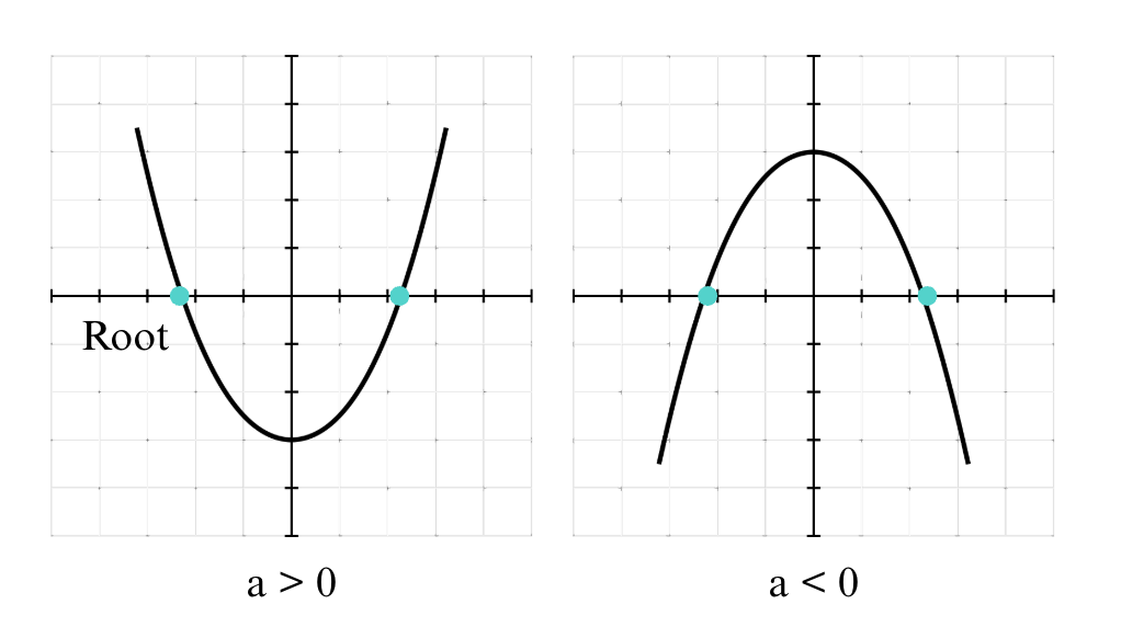
Thus, we always have , or if we restrict ourselves to positive definite matrices, and these typically appear anyway as part of our discretisation procedure. Therefore, we will always have a parabola that opens to the top (or a hypersurface in higher-dimensional space). Regardless of what type of abstract surface we are looking at, it will always open up to the top, and therefore, it will always have a minimum due to the positive definite restriction.
OK, so we have now derived all the math we need to understand why we can transform a linear system of equations into an equivalent minimisation problem. However, before we crack on with yet more linear algebra, I thought it might be good to look at a problem. I am going to purposefully select a simple problem with a 2-by-2 matrix. This doesn't have any relevance for CFD, unfortunately, but it does mean that we can look at the solution in a 2D space and visually see the equivalence between solving and minimising .
The example matrix I will be using is:
The right-hand side vector I'll be using is:
Since this example is so simple, we can compute directly if we wanted from . This means we have to form the inverse of , which we have avoided thus far like the pest. For larger systems, we don't want to invert , but for a 2-by-2 system, we should be OK. The inverse of a 2-by-2 matrix can be written as:
Inserting values, we get:
We can now compute the solution for as:
Thus, we now know that the solution should be . With that knowledge, let's evaluate the function of and see what happens. Remember, was given as:
Since we want to minimise this function, the constant is just going to raise or lower the minimum value, but it will not affect at which location this occurs. So, we typically set this value to and then we don't have to worry about it anymore (in-fact, we can remove it completely; it won't affect the solution we find).
The code below evaluates this function in the interval of and . This interval contains our solution , i.e. the solution is at and , and so, we should find a minimum of at that point. Here is the (Python) code with comments:
1 2 3 4 5 6 7 8 9 10 11 12 13 14 15 16 17 18 19 20 21 22 23 24 25 26 27 28 29 30 31 32 33 34 35 36 37 38 39 40 41 42 43 44 45 46 47 48 49 50 51 52 53 54 55 56 57 58 59 60 61 62 63 64 65 66 67 68 69 70 71 72 | import matplotlib.pyplot as plt import numpy as np # create 2-by-2 matrix A = np.array([[2, 1], [1, 2]]) # right-hand side vector b = np.array([5, 4]) # solving for x using x = A^{-1}b, which is cheap for a 2-by-2 matrix xsol = np.linalg.solve(A, b) # solution at [2 1] print('solution at ', xsol) # let's create a search space for f between -5 and 5 for both x and y # We know that the solution is at [2 1], which is within this interval xc = np.linspace(-5, 5, 100) yc = np.linspace(-5, 5, 100) # creating an empty array for f, where we store the solutions for f so we can plot it later f = np.zeros((len(xc), len(yc))) # the constant is not important, it will just shift our plane up or down # it won't have an effect, so we can set it to 0 c = 0 # compute for all values of x and y for i in range(0, len(xc)): for j in range(0, len(yc)): xvec = np.array([xc[i], yc[j]]) # change i,j to j,i indices here due to the difference in how indices # are interpreted in numpy and matplotlib f[j][i] = 0.5 * xvec.T @ A @ xvec - b.T @ xvec + c # create grid for surface X, Y = np.meshgrid(xc, yc) # create figure with 1x2 layout fig = plt.figure(figsize=(10,5)) # ---- LEFT: contour plot ---- ax1 = fig.add_subplot(1, 2, 1) cont = ax1.contourf(xc, yc, f, 50, cmap='viridis') # plot solution ax1.plot(xsol[0], xsol[1], 'rx') # dashed helper lines ax1.plot([2, 2], [-5, 0.7], 'r--') ax1.plot([-5, 1.7], [1, 1], 'r--') ax1.set_xlabel('x') ax1.set_ylabel('y') fig.colorbar(cont, ax=ax1) # ---- RIGHT: 3D surface ---- ax2 = fig.add_subplot(1, 2, 2, projection='3d') ax2.plot_surface(X, Y, f, cmap='viridis') ax2.set_xlabel('x') ax2.set_ylabel('y') ax2.set_zlabel('f') ax2.view_init(elev=30, azim=-30) plt.tight_layout() plt.show() |
This code plots two things at the end: a contour plot (i.e. a 2D projection of a 3D surface) and the 3D surface itself.
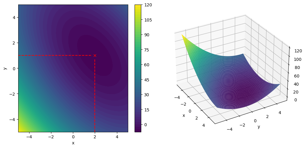
On the left, I show the contours of between and . I have shown, with a red cross, where the point and is located. These are the coordinates from the solution vector we have computed analytically (the code also computes this solution numerically as xsol = np.linalg.solve(A, b)). We can see, indeed, this is where the function appears to have its lowest function values, based on the colorbar.
I have also shown the surface in a 3D plot to the right. It is more difficult to see here that the minimum of this surface is indeed at and , but we can at least see that there is a minimum at this location.
What we can also see is that, indeed, we have a minimum, not a maximum, and so our matrix must be positive definite. We can check that for our solution vector and evaluate
Indeed, for this particular point, we have shown that , and you can insert any other vector , it will always give you a positive value. So, the matrix is not just symmetric (), but it is also positive definite.
Right, so we have spend quite a bit now on showing that we can minimise , instead of solving , so now we need to talk about algorithms to solve . And this is where we start to get towards the conjugate gradient method. But, before we do that, we will look at an intermediate method, which is known as the method of Steepest Descent.
The method of Steepest Descent
The method of Steepest Descent is, conceptually speaking, very simple. It is just difficult to visualise, unless we are dealing with a problem that fits into our 3D world. Just looking at the equations doesn't really build up an intuition, and so, we need to approach this from a 3D space initially. The good news is that this is not a limitation; the method generalises to higher dimensions by simply increasing the size of vectors and matrices.
That is, if we have a vector with 3 entries, then we can visualise this vector in 3D space. But, if we think of as being the solution vector of arising from a CFD problem, then this means that we have only three entries in our solution vector, e.g. we only have 3 cells in our mesh, and we store the solution inside each cell.
Typically, we have many more entries in , but if we have a mesh with 1 million cells, so that has 1 million entries, we can no longer visualise that, so we have to rely on the maths alone. But, what we derive works just as well in 3D space ( has 3 entries) as it does for a vector with 1 million entries. The maths is exactly the same; the only difference is the size of the vectors and matrices.
OK, now that we have established that, I want to go back to our function and try to minimise that. Let's develop our intuition and see how we can approach this problem.
Initially, I have no idea what the solution for is. The whole point is that I minimise , which then tells me what is. Thus, to start the algorithm, I have to pick a random value for . Any value will do. We may pick a zero vector, i.e. one where all entries are zero, or we may set equal to a solution computed from a previous timestep/iteration if available.
Once I have picked a starting location, I then need to find a way to update my location . A simple approach may be the following:
Here, is the updated location after one step. is the location at the previous step (or my initial guess if we are just starting the algorithm). is the direction in which we want to go, and tells us by how much we should be going in that direction, i.e. it is just a scalar multiplier.
Now we need to come up with some rules, i.e. how do we obtain the direction vector , and by how much do we multiply it. I'll propose a stupid algorithm (not to be confused with the STUPID turbulence model), which I will call "Tom is always right".
No, this is not a political statement; it tells us that we always have to turn right. So, after we have picked an initial direction (any direction, it can be a randomly generated vector), any subsequent vector we define has to point to the right. By how much? Well, if we now also generate a random scalar multiplier , we can evaluate Eq.(315) and get a new value for .
With this new value for , we can evaluate again, and, if this is smaller than the previous value of , i.e. obtained from , then we accept the randomly generated value for and right-pointing direction vector . The following figure shows one example of this direction, eventually finding the minimum.
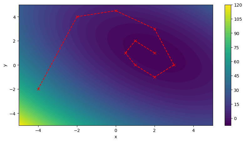
Now, of course, this is a stupid algorithm (I said as much), and there are many problems with it. First of all, our convergence rate is random. Run this experiment a few times, and you will get wildly different results. Secondly, we have to potentially evaluate many times before we accept a new direction, making the cost per iteration unpredictable. Thirdly, when do we stop? This algorithm will struggle to turn right close to the minimum of , and judging when this minimum is reached is not a trivial task.
The point is, with a simple line search algorithm, as given by Eq.(315), we can walk towards the minimum. In fact, this is exactly what the Conjugate Gradient method will do later (as well as the steepest descent algorithm). What differentiates both methods is how they determine the direction in which we go, as well as by how much we go in that direction, that is, the value for the scalar multiplier .
Clearly, we can do better than Tom's stupid algorithm, and thankfully, people with greater intellect before us have solved that issue for us already. This is where the method of Steepest Descent comes in. Let's have a look at a simple parabola , as shown in the following figure:
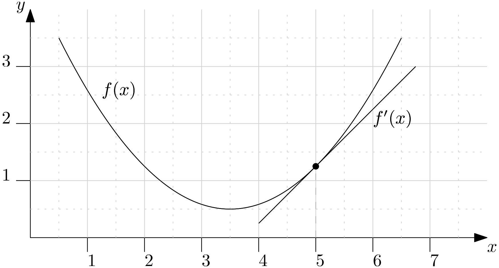
We have a random initial location given for (as indicated by the point at ), and we want to move to the minimum of . If we look at the derivative of , that is, , we see that the derivative is positive, i.e. . In fact, with the values provided, we can compute as . For example, evaluating the derivative between and , we get:
So, the derivative is indeed positive. But, if we walked now along the direction of the gradient, we would be going to the right (positive x-direction). This would take us away from the minimum. Instead, we go in the negative direction of the derivative, i.e. . By how much are we going in that direction (i.e. what is our scalar multiplier )? Let's simply take the absolute value of the derivative, i.e. . As we get closer to the minimum of , the derivative gets smaller and so our updated will get smaller as well.
We can now use Eq.(315) again, which becomes:
So, our new location is . We can now evaluate and get a new value for . Then, we can evaluate the derivative again, update again (where will now be , i.e. the value from the previous iteration), and we do that until we have (i.e. they differ by some small difference only). Eventually, we will get a value of .
For this simple function depending on only , we could stop here, but we need to now look at the 3D case (or, rather, the case where depends now on multiple directions). The Steepest Descent algorithm is schematically shown below:

Here, we have again some starting point which may be randomly guessed or given from a previous timestep/iteration, which is indicated by . We want to do a line search again, that is, along an arbitrary direction , we want to go along that direction until we hit a local minimum on the surface (along the direction of ). This will not be the global minimum of , but it will be the minimum along starting from , as indicated by the dashed line through .
Now comes a crucial step in the Steepest Descent algorithm: to obtain the next line search direction, we look for the gradient in a direction that is normal (at a 90-degree angle) to the previous search direction. This is shown by the dashed line going from to . We repeat our line search now by finding the local minimum on this new dashed line.
This algorithm converges very quickly to the minimum of , which makes it a very robust algorithm. The question is, how do we find our search direction and the scalar multiplier ? Well, let's have a look.
To start the algorithm, we need to find a starting point and a search direction . The starting point is simple; remember that represents our solution vector (e.g. our velocity, pressure, temperature, density, turbulent kinetic energy, etc.), i.e. it is the quantity we are solving for. When we start our simulation, we have to initialise our solution (for example, setting all values to the ambient values or values set at an inlet). So, when we start the simulation, is just our initial solution.
As the simulation progresses, we set equal to the solution we had at the previous iteration, though we could also set to anything we want, really. But setting it to the solution from the previous iteration means that we are probably already quite close to the minimum, and so, we will need fewer iterations to find the minimum.
What about the search direction ? Well, we can construct it from our linear system . We can bring onto our left-hand side, and have:
We saw this before, when we derived the function for . When we did that, we said the right-hand side is equal to the derivative of , i.e. if the derivative is zero, then we have found a local minimum. Thus, we have:
When we looked at the method of Steepest Descent, we said that we always want to go in the negative direction of the gradient (as we did in the figure above with the parabola). Therefore, we multiply this equation by and have:
And this is our search direction. We can write this a bit cleaner as:
Ok, so we now know what our starting point is, we know what the initial search direction is, based on the negative gradient of , but we don't know yet by how much we should go along our search direction , i.e. we need to find the scalar multiplier . To find that, we need to construct an equation for the search direction update, find a way to get into that equation, and then solve for it.
In the method of the Steepest Descent, we said that the next search direction should be at a normal angle (90 degrees) to the previous search direction. How can we express that? Well, let's take a simple example in 2D. If my search direction is , that is, along the x-direction, which vector would be normal to that? Well, if is along the x-direction of my coordinate system, a vector normal to that is the y-direction. So, we would expect our next search direction to be along the y direction.
It can either point along the positive or negative direction of y, i.e. and are equally possible, it depends on the gradient of where we evaluate . When we have two vectors which are normal to each other, as we have in this case, we know that their dot (or scalar) product is zero, that is:
We know that the dot product gives us the angle between two vectors using the cosine function, and the cosine of 90 degrees is 0, i.e. . So, if the dot product evaluates to 0, then the vectors are at a 90-degree angle to each other. We can use this to write our search directions as:
This statement enforces that a new search direction at is going to be normal to our previous search direction at . We have also seen that we can write this dot product in a slightly different form:
Here, we write the search direction at as a row vector, and the search direction at as a column vector. As we have seen previously, this product is the same as forming the dot product. I'll use this notation from now on, as this is how you will find it in the literature, but know that you can always replace it with the dot product if you want.
Remember what we want to do here, we want to find the scalar multiplier for the current search direction, i.e. we are still at iteration , so we don't think about updating our search direction yet. Therefore, we can use Eq.(324) now and see if we can construct an equation for .
We start by eliminating quantities we don't know. We don't know the search direction , and so we need to get rid of it. We already saw that the search direction can be computed from Eq.(321). In this equation, we didn't introduce indices for and yet, so let's do this first. We had:
If we want to express that as a search direction at , then we have
If we needed the search direction at , we could have equally set and at . However, with this equation given now at iteration , we can insert that into Eq.(324) and get:
Hmmm, ok, so we got rid of , but now we have the updated location at in the equation. We don't know yet where it is. The whole point of finding an equation for is that we can compute what will be. So, sorry, , you have to go as well. If we look back at our line search equation, i.e. Eq.(315), we had:
Ah, perfect, we can get rid of and, at the same time, replace it not just with an equation for , but also with all other quantities that are known in this expression. Cool, let's insert that then into Eq.(327). This gives us:
So, we now have an equation where all quantities are known, except for . This means we can solve the equation for and compute our scalar multiplier. We start by multiplying out the parentheses:
Have a look at the first term on the left-hand side, we have . This is nothing else than our search direction, or residual, at iteration , i.e. . Thus, we can simplify this equation as:
Now let's have a look at the right-hand side. When we have a matrix vector product, i.e. , it produces a column vector (for example ) as:
Then, we have to take the transpose of , i.e. , and multiply that by , i.e.
Again, a row vector multiplied with a column vector is just the scalar product. So, we can also write . Since multiplication is commutative (the order of multiplication does not matter), we can write . Writing this again as a row and column vector multiplication, we have:
We can insert this result back into our equation for , i.e. Eq.(331), which gives us:
Now we divide by and obtain an equation for as:
Even though we have now vectors and matrices in the numerator and denominator, these will all evaluate to scalars, so that will remain a scalar.
You might still be hung up on why we bothered to waste our energy to replace with . Why did we do that? Was there any point? No, not really, but this is, again, how you will find introduced in the literature. I am sure whoever came up with this form was just flexing, wanting to show how well they can manipulate linear algebra equations. But there is no need to do so, we could have just as well written:
We can also get rid of the row vectors now (transposing our column vectors) and write everything as dot products:
Or even:
All of these equations for are equivalent, and we can use any of them, but if you open a CFD textbook, you most likely will find given as:
This is our final result for alpha. Now that we have , , and , we can update our solution using the line search algorithm as:
We repeat this until , where we have to specify a suitable tolerance (e.g. , something small). Or, we just let it run for a few iterations and hope it converges. Ah yes, there it is again, hope ...
Thus, we can formulate the Steepest Descent algorithm as follows:
- Set from the initial solution or previous timestep/iteration.
- Compute a search direction .
- Compute the scalar multiplier
- Find a new solution using the line search algorithm .
- Go back to step 2 and repeat until , or until the maximum number of iterations has been found.
To show you how simple it is to implement the Steepest Descent algorithm, have a look at the following Python implementation using numpy (if you are not familiar with numpy, think of @ as a vector-vector and matrix-vector multiplication operator):
1 2 3 4 5 6 7 8 9 10 11 12 13 14 15 16 17 18 19 20 21 22 | import numpy as np import matplotlib.pyplot as plt A = np.array([[2, 1], [1, 2]]) b = np.array([5, 4]) xnew = np.array([-4, -2]) solutions = [] solutions.append(xnew) for k in range (0, 5): xold = xnew r = b - A @ xold alpha = r.T @ r / (r.T @ A @ r) xnew = xold + alpha * r solutions.append(xnew) # print solution table print('iter | x | y |') print('-----|--------|--------|') for k, x in enumerate(solutions): print(f'{k+1:4d} | {x[0]:6.3f} | {x[1]:6.3f} |') |
The code produces a table at the end to show the values of the new solution we compute. The table is shown below:
1 2 3 4 5 6 7 8 | iter | x | y | -----|--------|--------| 1 | -4.000 | -2.000 | 2 | 1.041 | 2.033 | 3 | 1.905 | 0.953 | 4 | 1.985 | 1.016 | 5 | 1.999 | 0.999 | 6 | 2.000 | 1.000 | |
The first iteration is our starting point, i.e. let's say that our solution at the previous timestep/iteration was . Then, after only one iteration, we have found a pretty good solution already. I am running this algorithm here for 5 iterations. I am not checking if , because I wanted to show you how quickly this algorithm converges.
Now, think about it for a second. We started with . What we want to do is find a solution for . The naive approach would be to form the inverse of and multiply both sides by it, which would give us: . But, as we saw, inverting the matrix, using Gaussian elimination, for example, takes too long.
OK, then, in our quest to finding a better algorithm, we looked at LU decomposition, which still uses Gaussian elimination, but stores the result in such a way that we can reuse it. But even LU decomposition was too slow. Then, we looked at iterative methods, like the Jacobi and the Gauss-Seidel method. While we did not use them to solve a system of linear equations, I said that they are typically very slow to converge, with Gauss-Seidel converging about 2 times faster than Jacobi.
But now, we have arrived at the method of Steepest Descent, where within a single iteration, we get a pretty good estimation of the final solution. After only 5 iterations, we have found pretty much the exact solution. And, even if our initial guess for is far off, this method still converges rapidly. For example, if we multiply our initial solution by a factor of 100 (we have ), then this is the table for 5 iterations (the first iteration being the initial solution):
iter | x | y |
-----|--------|--------|
1 | -400.0 | -200.0 |
2 | -62.25 | 70.20 |
3 | -4.355 | -2.177 |
4 | 0.984 | 2.094 |
5 | 1.900 | 0.950 |
6 | 1.984 | 1.017 |
While we don't get perfect results after 5 iterations, we would likely converge within a few extra iterations. Thus, not only is this method rapid, but it is also pretty insensitive to the initial condition.
But let's go back to our first example, where we started at . We can visualise the solution vector at each iteration and show how the Steepest Descent converges quickly towards the global minimum:
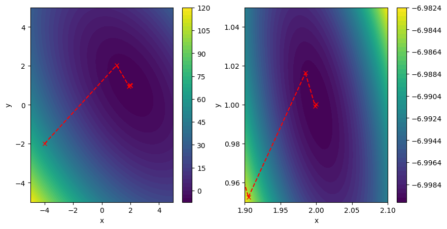
You might be saying, "Well, didn't we say that the Steepest Descent algorithm takes search directions at a normal angle?" Yes, we did say that, but we only used that as a condition to derive . We never actually enforced this condition when we compute a new search direction . Instead, we simply evaluated the residual at the beginning of each iteration and set . That was all.
As a result, we don't get perfectly orthogonal (normal) search directions. As it turns out, the Steepest Descent algorithm does indeed find the local minimum quickly, but, close to the minimum, it tends to oscillate. Once the method is within the vicinity of the exact solution, it struggles to converge. It's like a sprinter who can do the first 90 meters blisteringly fast, but struggles on the last 10 meters in a 100-meter sprint.
If you go back to our example where we started at , we look at how the solution for the y-coordinate oscillates around the exact solution of 1. It does eventually find it, but there are oscillations. These oscillations arise as we limit our new search direction to be orthogonal to our old search direction. This brute force approach works well if we are far away from the minimum. Close to the minimum, however, things change. Here, we need a different strategy to get quicker convergence.
Summary of the Steepest Descent method
In summary, the Steepest Descent method can be written down as follows:
- Loop from to
- Compute residual:
- Compute search direction length:
- Compute new position on : .
- Compute residual: or
- If or , break, otherwise, go back to step 2.
- End
Issues with the Steepest Descent method
Let's investigate why the Steepest Descent algorithm struggles near the minimum. To do that, I have created two surfaces and visualised the search path of the Steepest Descent algorithm on both. This figure is shown below:
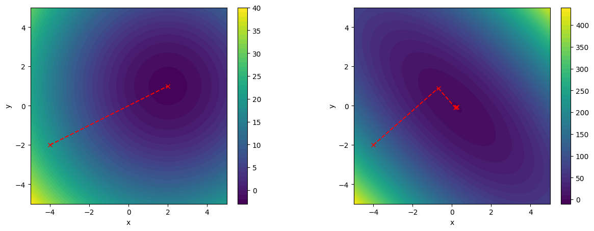
For both surfaces, I am using a right-hand side vector of , and a starting vector of . However, the coefficient matrix is different in both cases. For the left and right surfaces, I am using the following matrices:
Let's first try to link the matrices back to what we can see in the figures. The left matrix is the identity matrix. Crucially, it does not have any off-diagonal entries and only the main diagonal contains entries. The surface that we are getting is producing perfectly round iso-contours. What does that mean? Well, at any given point on this surface, if we take the derivative, it will point straight to the minimum.
How about the matrix for the right figure? It does contain off-diagonal elements, and these introduce stretching. These off-diagonal entries stretch our otherwise circular iso-contours to elliptical iso-contours. So, how can we link this now to the performance of the Steepest Descent algorithm? Let's look at the following sketch:

Here, I show a circle and an ellipse, and I have drawn tangents at an arbitrary point along the circle and the ellipse. If we take the gradient at the intersection of the tangent with the circle and ellipse, it will point in a direction that is normal to the tangent. We can see that this points straight to the center for the circle, and, it doesn't matter where we were to draw the tangent; the normal to any tangent will always point to the center of the circle!
But how about the ellipse? Well, certainly, there are some places where the normal to a tangent points straight to the center, as shown on the far left of the ellipse. But, these are exceptions, and in most cases, the normal to a tangent (the derivative) points to a location away from the center.
As a result, if we use the Steepest Descent method on a surface without any stretching (the matrix only contains diagonal entries), then finding the minimum is quick. But, once we have stretching (off-diagonal entries), the Steepest Descent method struggles to point to the center of the surface. And, the stronger the stretching, the worse the performance of the Steepest Descent algorithm gets.
We can also show this mathematically. We looked at it earlier in this article in Eq.(62), repeated below for convenience.
This depends on the eigenvalues. Since our matrices are 2-by-2, we can quickly evaluate the eigenvalues. For the left matrix, we have:
Since we have a 2-by-2 matrix, we expect two eigenvalues. However, there is only one eigenvalue that satisfies and that is . Therefore, we have . What does that mean for our condition number? We have:
When we discussed the condition number briefly, I mentioned that the closer the eigenvalues are together, the faster the convergence will be. In this case, all eigenvalues (well, all two of them) are exactly the same, and so, we would expect fast convergence. Indeed, looking at the figure above, where we see the surface and the path of the Steepest Descent algorithm, we can see that it converges within a single step.
This is because has no off-diagonal entries, and so its contours are perfectly circular, and so no matter where we are on the surface , the gradient will always point in the direction of the center, as we have established by looking at the circle, its tangents and the normals to the tangents.
Now, let's compute the eigenvalues for the second matrix. Here, we have:
From this, we can now compute to be:
Using the abc formula, we can find the roots of this expression to be:
Thus, we have and . What does that do to our condition number?
Due to the off-diagonal entries, we now get stretching on our surface , and this increases our condition number. A larger condition number means we have to wait longer for the algorithm to converge, and, in the case of the Steepest Descent method, we see that this is because the method has to now zig-zag to the minimum. The stretching means derivatives point no longer to the minimum everywhere on the surface, necessitating this zig-zag approach.
If I borrow the Poisson equation again, which we solve, for example, for an incompressible flow (SIMPLE, PISO, Pressure Projection methods), then we can see how these matrices with off-diagonal elements (and thus stretched surfaces ) come about. The Poisson equation for the pressure may be discretised as:
We can also write this in matrix form as:
If we set for simplicity, then we can compute our coefficients as and . Our coefficient matrix becomes:
It is a symmetric and positive definite matrix. Crucially, what we can take away from this is that if the stencil of our numerical scheme is symmetric, then our coefficient matrix will be symmetric as well. That is, if our numerical scheme uses , we require that we also use , and the coefficients for both and have to be the same (these will become the entries on the off-diagonals, i.e. and ).
So, for example, if we used an upwind scheme, it will not use a symmetric stencil, that is, we use either values from or in our discretisation, but never both sides. And, since our momentum equations are typically discretised with some form of upwind schemes, we typically have non-symmetric coefficient matrices for our momentum equations and thus can't use the Conjugate Gradient method here.
I should clarify here that even if we don't use the upwind scheme directly, other popular schemes like MUSCL and WENO are all based on the idea of upwinding (i.e. their stencil adjusts based on the direction of the flow).
Returning to our Poisson equation coefficient matrix, if we make this a specific, 2-by-2 matrix again, and compute the eigenvalues for this matrix, we get:
We can again compute as:
Using the abc formula as before, we can find the roots as:
To compute the condition number (which is always positive, that is just its definition), we have to take the absolute values of our eigenvalues, so we get and . The condition number is then found to be:
So, we can see how a typical example from a pressure Poisson solver, which we frequently use in CFD, especially for incompressible flows, results in matrices that are not ideal for the Steepest Descent method. This is where the Conjugate Gradient method shines, so let's have a look at it next.
Putting all together: the Conjugate Gradient method at last
Let's approach this problem like an engineer. We need to establish what works really well for the Steepest Descent method, and what doesn't. We retain the favourable properties and try to improve upon the weaknesses.
The Steepest Descent method gets us to the minimum quickly. This is really good, and we would like to use that in our Conjugate Gradient method. However, once we are close to the minimum, it starts oscillating, so the search direction update is not ideal. We want to improve that.
So, we need to consider how we can obtain in a better way. To do that, let's consider the following figure:
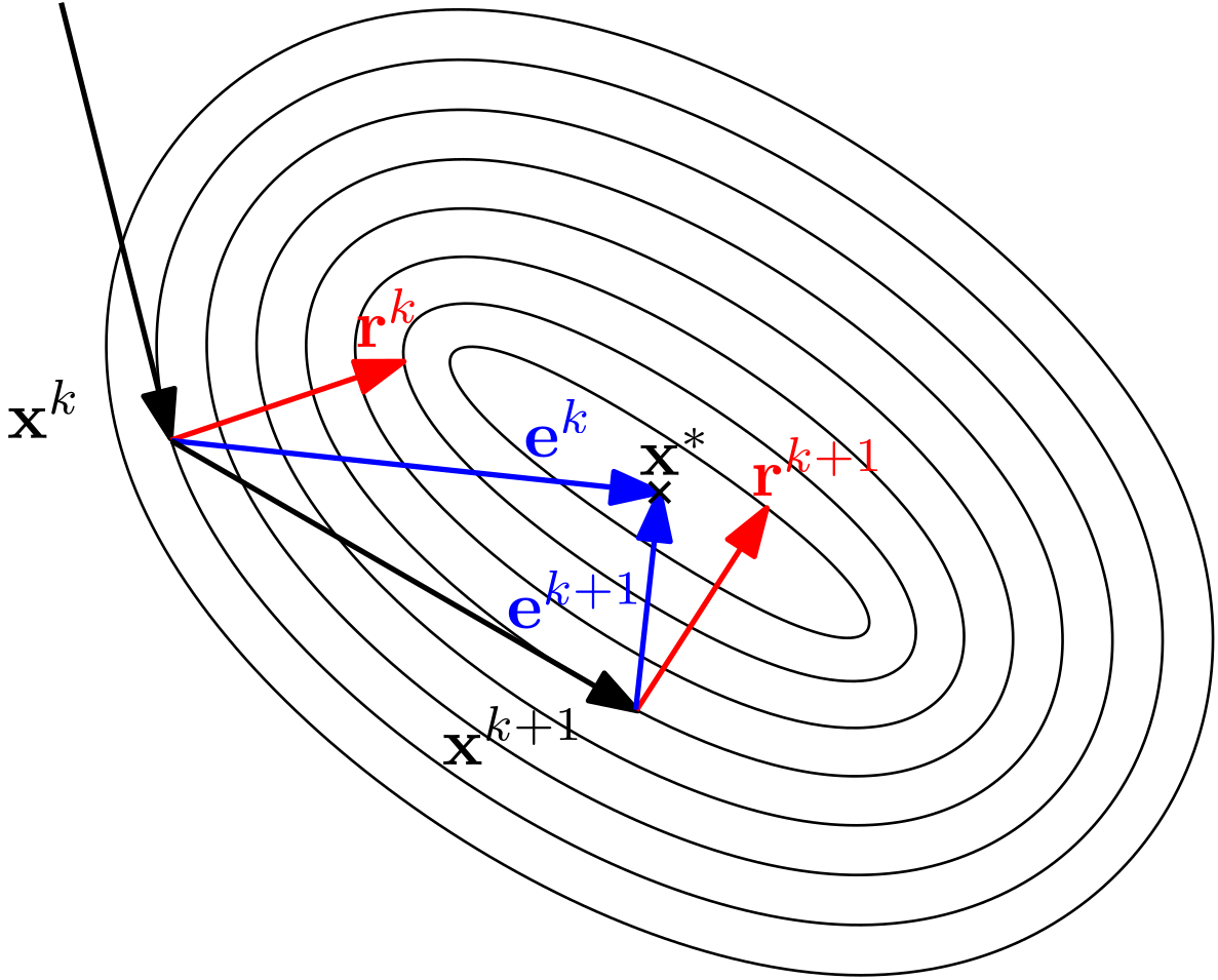
Here, is a possible location we have obtained on our surface after trying to get close to the minimum. is the location at the next iteration. For both positions and , I have also shown the direction vector and in red, which are orthogonal/normal to and . This is the direction we would go in the Steepest Descent algorithm.
In blue, I have shown the direct path from and to the center of the surface , indicated by the labels and , and it is this direction we ideally would like to take, but we don't know how to get these directions. But, we can express them mathematically as:
Here, is is the location where has its minimum, as indicated in the figure above as well. That is, the is the location we want to find to get our solution vector . Therefore, we can also interpret as the error between the current location and the location where has its minimum.
As we can see, and are not necessarily orthogonal to each other. In the Steepest Descent algorithm, we just say that we pick the next search direction to be orthogonal to the last one, which will guarantee that we will find the minimum eventually, even if it oscillates near the minimum.
In the Conjugate Gradient method, however, we want to try to get closer to the minimum, and so we want to move as close as possible in the direction of as possible.
Now, let us try to build up some intuition before we go to the next step. We said that if we had an identity matrix, the Steepest Descent method would converge rapidly. It does so; no matter where we take the gradient, it will always point directly to the minimum of the surface.
Only when we start to stretch the surface, by introducing off-diagonal terms in our coefficient matrix , does the Steepest Descent method start to stutter and provide a zig-zag approach to find the solution. So, this leaves us with two possibilities:
- If we want to continue to use the Steepest Descent algorithm as it is, then we first need to transform our surface into a space where our surface that we seek to minimise becomes non-stretched.
- If we want to leave the surface as it is, we need to change our search direction, and it should include our coefficient matrix , so that the stretching of the off-diagonal terms influences the search direction.
Let's look at both methods in turn. For the first possibility, we need to transform our surface into a non-stretched version. We said that the surface is stretched because of our coefficient matrix , which has off-diagonal components. So, if we wanted a non-stretched surface , what we need is a matrix that is ideally an identity matrix. And how do we construct an identity matrix from a given coefficient matrix? Well, we have the following definition:
So, if we have given, all we need is its inverse , and we can construct an identity matrix. We can then multiply our surface by and have an easy problem to minimise, where the Steepest Descent method will converge rapidly. But, if we have given, well, then we can solve explicitly as:
So, yes, while technically this approach would work, it is the nuclear option, and it won't help us. We try to avoid having to solve for , and so a transformation of is off the table.
Let's look at the second approach, where we said that we keep as it is, but we try to incorporate into our search direction.
In the Steepest Descent algorithm, we said that our search directions and should be orthogonal to each other, so that we have:
Now we want to insert into this expression. As we have seen before, a matrix multiplied by a vector is going to be a vector, so if we replaced by , we still have a vector. Let us insert that into our search direction update, and we get:
We said that Eq.(360) shows orthogonality between and . In analogy, we say that Eq.(361) shows A-orthogonality, that is, and are A-orthogonal to each other. Instead of using the word A-orthogonal, we can say that and are conjugate to each other. This is where the first part of the name Conjugate Gradient comes from.
Now we do one more step. In Eq.(361), we replace by . We don't know what is, but we can try to eliminate it by constructing equations from known quantities that relate to . We do that because points directly to the minimum of , and so, if we can find an equation for , even just an approximation, we should be better off than with the Steepest Descent algorithm.
Thus, our vectors become:
Let's look at that visually. We can visualise the difference between and as follows:
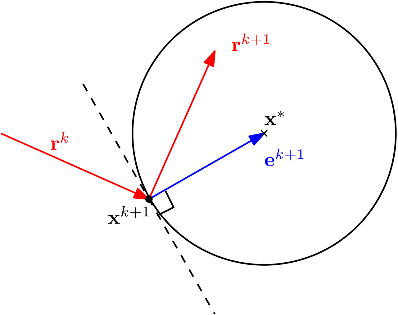
We can see the search direction that brought us to , i.e. the red arrow . Once we reach , we can see that the next search direction is in the Steepest Descent, being orthogonal to . This does not get us to the minimum. But what about ?
I have shown here a circle with its center at which intersects . I have also shown a tangent to the circle, and we can see that is normal (orthogonal) to the circle's tangent at . Thus, for any given point , represents the shortest distance to the minimum. Therefore, the expression gives us the shortest direction from to .
This is the main difference between the Steepest Descent method and the Conjugate Gradient algorithm. The only thing left for us to do now is to derive an expression for . Whenever we are tasked with a problem of expressing an unknown property (e.g. ) by known properties, it helps to write out all of the equations that we do know for the unknown property. So let's do that. We already stated that we can express as:
We also know from the Steepest Descent algorithm that we use a line search to update , i.e. Eq.(315), which was given as:
We now change to to indicate that we use an independent search direction in the conjugate gradient method. Thus, our line search becomes:
If we now subtract from both sides, we get:
We also know that once we have found the exact solution , it must satisfy our original problem:
However, if we are still looking for a solution, and , we know that there will be a residual, that is:
This residual was used as the starting direction for the Steepest Descent algorithm. Since the right-hand side vector can be expressed as , we can insert that into the previous equation and get:
Now we can use the definition for again, which was: . Here, the subtraction is the other way around compared to the previous equation. So, we can multiply the previous equation by and get:
Now that the subtraction is the same as in , we can insert and get:
By the same logic, we can also derive an equation for the error at . We start with the residual at :
Then, we insert for and get:
We multiply again by :
We can insert and get:
With these definitions, we can now attempt to find the scalar multiplier (i.e. the search distance). We start with our conjugate vectors:
Here, I have replaced by . I did that because our goal is to find a search direction that is different to the one taken in the Steepest Descent. However, as we will see later, at our first iteration, we have , that is, in the first iteration, both are the same.
However, the Conjugate Gradient method will provide us with a mechanism to independently tune our search direction so that it points closer to the minimum of , and so, we need to distinguish now between the search direction and the residual (which was used in the Steepest Descent as the search direction as well).
The first step is to eliminate . We saw that this can be expressed as from our line search approach. So, let us insert that for . We get:
Since we have already shown that , we can insert this as well into our equation and get:
Now we divide by and get:
Thus, our scalar multiplier becomes:
To start the calculation of , as already alluded to before, we set and at the first iteration, i.e. (or if you must use Fortran, my condolences ...). In this way, we can compute .
If we left it at that and set , well, then we would have created the Steepest Descent algorithm again, but clearly this isn't our goal. So, we need to now look at how we can update the new search direction independent of .
So, let's remind ourselves what equation we already have that we can use to construct . We will make use of Eq.(375) and Eq.(376) to begin with, which are repeated below for convenience:
Inserting into results in:
We can also write this as:
Now we multiply both sites by and get:
So, the search direction at is orthogonal to the residual at the next iteration . Let's look at this schematically. The following figure shows how, at , the search direction is orthogonal to at :
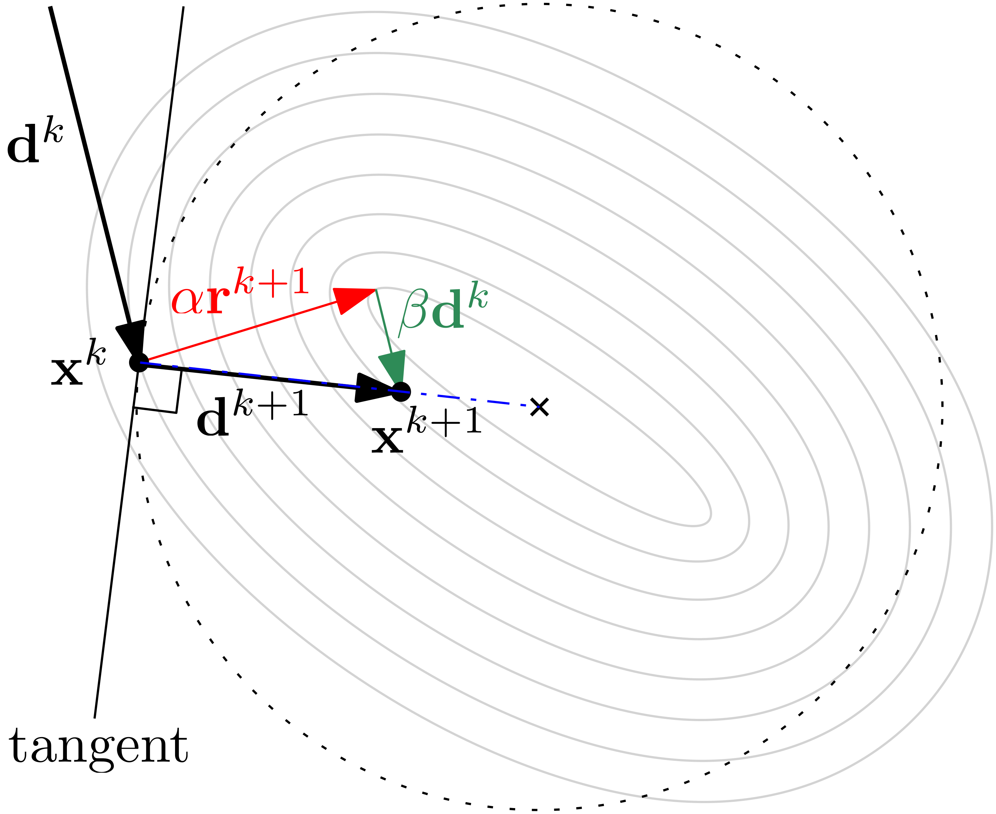
The vector may have any length, but I am showing it here multiplied by , so that it reaches the local minimum along that search direction. We know that the location reached by is the location where the Steepest Descent method would send us. In the Conjugate Gradient method, however, we go introduce a correction now, that is in the same direction as the old search direction, i.e. , and we multiply that by some unknown scalar multiplier .
The goal of , as we can see, is to correct the new search direction so that it points towards the minimum of the surface . This is shown by the pointing in the same direction as the dash-dotted line, shown in blue, which we introduced as the error , i.e. the distance between and the location of the minimum of . If would get us all the way to the minimum of , then we would have .
But, as we are not guaranteed to move all the way to the minimum of , but instead only a fraction of , they are not the same. But, since we are moving at least in the direction of , we hope to achieve faster convergence compared to the Steepest Descent method, or, at the very least, to avoid oscillations near the minimum.
OK, so far, we have yet again shifted the problem of finding a new search direction by expressing it through a new unknown quantity, in this case, . Let us write an equation for first, and then see how we can obtain . Based on the previous figure, we can express the new search direction as a combination of and as:
Note: I have removed here from the equation. But that is not an issue, or a simplification. If the length of changes, we simply have to change the distance of so that we are still arriving on a point somewhere on the blue dash-dotted line. Essentially, is just determining how large the triangle is that is spanned by , , and .
Now let's look at in the figure above. You can see that I have drawn a dotted circle around the center of the minimum of . I have also shown the tangent at , and we can see that the new search direction is orthogonal/normal to that tangent.
As we have discussed before, we can say that is A-orthogonal, or conjugate, to . We can express that as:
Now, let's try to combine that somehow with Eq.(385). In this equation, we know the right-hand side, except for . However, we don't know the new search direction . So, we have two unknowns in this equation. Since we want to determine , we need to get rid of the new search direction .
If we were to multiply Eq.(385) by , then the left-hand side of Eq.(385) would become . From Eq.(386), we know that this is zero, and so we can effectively eliminate , and so reduce the number of unknowns in Eq.(385) from 2 to 1.
So, let's do that. Let's multiply Eq.(385) by and we get:
We divide this equation now by and get:
We can solve this for now and get:
Knowing what is, we can now determine the new search direction as:
This is it, this is the method of the Conjugate Gradient method. I have already talked a few times about where the conjugate part is coming from in the name, but what about the gradient part? We saw that we start the Conjugate Gradient method just like the Steepest Descent method, and then correct the search direction. But, at the very first iteration, we set the search direction equal to the residual .
This is coming from the Steepest Descent method, and, since is pointing along the gradient, so will at the first iteration. So, our starting direction points along the gradient at whichever point we are starting at. Hence, since we go initially in the direction of the gradient but then take conjugate, nor orthogonal search directions, we end up with the name Conjugate Gradient.
We could leave things here and move on to the next topic, but if you look at the Conjugate Gradient method in the literature, you will see a slightly different formulation for . In Eq.(389), we had:
An entirely equivalent expression is:
It is just a reformulated version of . Why do we prefer the second version? Because it does not have any matrix-vector multiplications, only scalar products (or vector-vector multiplications). Thus, the second version is much cheaper to evaluate.
Shall I use the same CFD textbook approach and say it is easy to see that Eq.(392)follows directly after some manipulation of Eq.(389)?
Nah, I'd like to derive my equations in full. For me, it is not easy to see that Eq.(392) follows from Eq.(389) without seeing the derivation.
We start by deriving a useful relation that we will need in a bit. We know that the residual at iteration and can be written as:
We also know, from our line search algorithm, that a new position on the surface at , i.e. for the next iteration, can be found as:
We now insert into our equation for the residual, i.e. and get:
We can expand the parentheses and multiply by each term. This gives us:
I have shown that the first two terms combined are nothing else than the residual at iteration , i.e. . Therefore, we can write this also as:
We can now rearrange this equation by bringing onto the other side and get:
Let's multiply by to get rid of the negative sign:
As a last step, let's divide by :
And, just to make it easier for ourselves later, let's also swap sides:
Good, we will need this result in just a bit. Returning to the equation of , we had:
In the following derivation, we will find equivalent expressions for both the numerator and denominator .
Let's start with the denominator, i.e. . We can find an equivalent expression from the scalar multiplier . This was given as:
Multiplying by we get:
Dividing by we get:
Let's take that in for a second. The left-hand side shows , i.e. the denominator for the expression of . But the right-hand side shown an expression that only depends on a single scalar product (or vector-vector multiplication). This will cost less computational effort to evaluate.
Great, now moving on to the numerator . Since is symmetric, we have . We can use this identity to write the numerator as:
Now we can use the rules of transposition. For two generic matrices (of which one can also be a vector as long as the dimensions match) and , we have:
Thus, we can use this rule for and write this as:
Therefore, the numerator becomes:
Now we use Eq.(401), which we derived earlier and which was given as:
First, we take the transpose of both sides:
We multiply that by and get:
We can see that the left-hand side is equivalent to Eq.(409)'s right-hand side, so we can substitute:
We now expand the parentheses on the right-hand side and get:
Now we use the identity that the Conjugate Gradient method inherits from the Steepest Descent method. That is, subsequent residuals are orthogonal to each other:
Remember, in the Steepest Descent method, we then use as the new search direction, whereas in the Conjugate Gradient method, we correct this so that the new search direction is conjugate (taking the coefficient matrix into account). For that reason, we have a separate search direction from the residual, though the property that is still present in the Conjugate Gradient method.
Therefore, we can eliminate from Eq.(414) and get:
OK, so, to summarise, from Eq.(405) and Eq.(416), we have gotten the following identities:
We can now insert these into our definition for , i.e.:
Doing so, we get:
The cancels, and the two minus signs become a plus sign, so we can simplify this as:
Indeed, we have now found an expression for that does not require any matrix-vector multiplications. Horray! Once we have , we can compute the search direction at , which is conjugate to at iteration . We have:
So, just like in the Steepest Descent method, let us implement the Conjugate Gradient method and see how it performs. We take the same surface , i.e. the same coefficient matrix and right-hand side vector . We also start from the first initial location . Here is the implemented algorithm in Python again, using numpy:
1 2 3 4 5 6 7 8 9 10 11 12 13 14 15 16 17 18 19 20 21 22 23 24 25 26 27 28 29 30 31 | # conjugate gradient import numpy as np import matplotlib.pyplot as plt A = np.array([[2, 1], [1, 2]]) b = np.array([5, 4]) xnew = np.array([-4, -2]) solutions = [] solutions.append(xnew) dnew = b - A @ xnew r = b - A @ xnew for i in range (0, 5): xold = xnew dold = dnew r = b - A @ xold alpha = dold.T @ r / (dold.T @ A @ dold) xnew = xold + alpha * dold rnew = r - alpha * A @ dold beta = rnew.T @ rnew / (r.T @ r) dnew = rnew + beta * dold solutions.append(xnew) # print solution table print('iter | x | y |') print('-----|--------|--------|') for i, x in enumerate(solutions): print(f'{i+1:4d} | {x[0]:6.3f} | {x[1]:6.3f} |') |
On lines 12 and 13, we can see that both the initial residual and search direction are equivalent at the start of the algorithm. Thus, lines 16-18 are just the Steepest Descent method. On lines 20-22, we do our correction to the search direction, so that dnew and dold, i.e. the search directions at and are conjugate to each other.
This algorithm provides the following results:
1 2 3 4 5 6 7 8 | iter | x | y | -----|--------|--------| 1 | -4.000 | -2.000 | 2 | 1.041 | 2.033 | 3 | 2.000 | 1.000 | 4 | 2.000 | 1.000 | 5 | 2.000 | 1.000 | 6 | nan | nan | |
We have found the correct solution within 3 digits after only 2 iterations! Compare that with the results we obtained from the Steepest Descent method. There, we had the following table:
1 2 3 4 5 6 7 8 | iter | x | y | -----|--------|--------| 1 | -4.000 | -2.000 | 2 | 1.041 | 2.033 | 3 | 1.905 | 0.953 | 4 | 1.985 | 1.016 | 5 | 1.999 | 0.999 | 6 | 2.000 | 1.000 | |
While the Steepest Descent method also converged to within 3 digits after 6 iteration, it took 3 times longer than the Conjugate Gradient method to get there. And, in comparison to the Conjugate Gradient method, we can clearly see the typical behaviour of the Steepest Descent method, which is that it oscillates near the minimum of .
There is one more thing: After 6 iterations, we get nan for the Conjugate Gradient method. Now, why is that? Referring back to the code, if we run this with debug information available and step through the code, we will find that, after a few iterations, will evaluate to nan.
It does so because it has a division by , i.e. the residual. After only a few iterations, we are so close to the minimum of so that the residual becomes effectively zero (to within machine precision). Therefore, we have division by zero, which sets equal to nan, and then, all values multiplied by also become nans.
This is yet another indicator that the Conjugate Gradient method converges extremely fast. In reality, we would check if and stop the method before we get division by zero. I just wanted to show how quickly we get to the correct solution (minimum of ) and how that compares against the Steepest Descent method.
Let me leave you with this analogy, comparing the Steepest Descent method with the Conjugate Gradient algorithm.
I don't play golf (I suppose for the same reason as Franky Boyle), but the golf ball is one of those things we can't avoid in fluid mechanics. It is often used to explain the favourable properties of turbulent boundary layers and how they can actually decrease drag (which, the Mythbusters put to the extreme to build a dimpled, golf ball-like car to reduce drag), as they carry more energy than laminar boundary layers.
Be that as it may, even I know that a golfer has different clubs available at their disposal. You would use a driver to get the golf ball as close to the green (where the hole is) as possible. The driver gives you a good distance, but not good precision. Once you are on the green, you want to use a putter, which doesn't give you distance, but precision instead.
The Steepest Descent method is like a driver; you can be as far away from the function's minimum (i.e. the green/hole in this analogy) as you want, the Steepest Descent algorithm will get you very quickly into the vicinity of the minimum (i.e. the green). The Conjugate Gradient algorithm uses the same approach as the Steepest Descent method initially for exactly that reason; fast convergence towards the minimum of .
Once our golf ball is on the green, a golfer would now switch to a putter, which trades precision for distance. We won't get the golf ball far, but we have a lot more control over its direction of travel.
In our analogy, the Steepest Descent method is like continuing to use a driver, even once we are on the green. The Conjugate Gradient method is like a putter, as we continuously correct our direction of travel, and so, we have more control (precision) on getting the ball into the hole (finding the minimum of ), and therefore converge faster (having a lower handicap).
It's good to see that all of that Nintendo Wii sports resort golf training wasn't in vain ...
OK, thus far, we have made the restriction that all of our matrices ought to be symmetric, but that really means all we can do is solve pressure Poisson equations, or heat diffusion type equations, with the Conjugate Gradient method. We can't use it for the momentum equation (unless we employ a symmetric stencil for our non-linear term, and there really is only one scheme that comes to mind that provides us with this property; the JST scheme). What if we wanted to generalise the Conjugate Gradient algorithm?
Well, fear not, others have done exactly that for us so that we can use the Conjugate Gradient method for non-symmetric matrices as well, and by far the most popular variant (there are several) is the Bi-Conjugate Gradient (Stabilised) version, or BiCGStab/BCGS, depending on which literature/software packages you use. We will review this method in a second as well. But first, let's summarise our Conjugate Gradient method, so that we have an easy cheat sheet should we need to implement it in the future.
Summary of the Conjugate Gradient method
In summary, the Conjugate Gradient method can be written down as follows:
- Loop from to
- Compute residual:
- Compute search direction length:
- Compute new position on : .
- Compute new residual:
- Compute correction along :
- Compute new (conjugate) search direction:
- Compute residual: or
- If or , break, otherwise, go back to step 2.
- End
Interlude: The Conjugate Gradient algorithm and the Krylov subspace
Remember our friend Krylov? We spent a lot of time looking at what the Krylov subspace is and how it is constructed. It is time to return to Krylov and look at why the Conjugate Gradient method (along with the Steepest Descent method and those that we are yet to review in this section of the article) are said to be Krylov subspace methods.
To do that, let me take you on a journey. On occasion, I have mentioned that I am very much German, and that is true, I was born and raised in there. However, having both German and Norwegian parents, I am technically speaking half-German and half-Norwegian (noen andre nordmenn her?).
In any case, as a result, I have spent lots of my summer holidays in Norway, visiting family, and one place in particular: Narvik. It's a small city above the northern polar circle, which makes it perfect to see northern lights in winter (which I was lucky enough to see a few times). In summer, though, the sun never sets, and you can enjoy a midnight swim in the Fjord. Here is an aerial view of Narvik:

You see the town at the base of the mountain on the left. Ignore the airport on the bottom left, which has long closed now (much to my annoyance, I never got a Saba-style landing in my life ...). The mountain on the right is what we are interested in.
Whenever I visited Narvik as a child/teenager, I would scale the mountain at least once, but often times more than that. My uncle, who is very much into Mountaineering, took me on a 1 week tour through Norway, trekking and climbing some of the larger peaks in the south.
This trip culminated in us sleeing in a hut that was officially ranked Norway's heighest building (build ontop of a mountain of about 2200 meters). They had bunkbeds, and I was the only one sleeping on the top, so, for at least a night, I was Norway's highest person (pun intended).
So, even though climbing mountains was not one of my active hobbies (that was a pretty difficult hobby to exercise for someone living in northern Germany, where the highest peaks around would be some landfills full of garbage and recultivated to look pretty), it is fair to say that I had a general interest in it.
So, imagine my delight when we went on a trip to Leines one day, and I was greeted with a mountain that was yet to be climbed by me: the Kraktindan:

We actually came here quite a few times, and I was always looking at the mountain, wanting to climb it at least once. But, every time we came, it was raining, or it rained the day before, and the trail was no good. But then, one day, a golden opportunity presented itself. The weather was cloudy, but no rain was forecasted. The trail was in good shape, and so I ascended to the peak.
I didn't know back then that this mountain in particular had a bit of a reputation. No one warned me about it because, well, I didn't really think to tell anyone that I was going there. I think I left a message before leaving, and off I went. The ascent was not too bad, and I must have reached the peak within two or three hours. It wasn't a massive mountain, and as long as you could see the peak, you knew where to go.
But then the mountain showed me why it had developed a reputation amongst locals, and why you should, perhaps, go a bit better prepared, like, havig a map, or even better, a GPS with you (we are talking about the early 2000s here, smartphones did not exist yet and the best part about my mobile at that time was Snake 2).
While it was cloudy for the whole duration of the ascent, once I reached the peak, I realised that I was very close to the clouds. I took a bit of a break, taking in the view, and, without much of a warning, the cloud cover descended, and all of a sudden, there was a 5-meter visibility at best. While some footpaths existed near the base of the mountain, there were no clear paths near the peak.
So, here I was, no map, no GPS, no compass, only me and my teenage ignorance of the Norwegian climate. I decided, perhaps it was time to go back home, but where to go? I knew roughly which way to go, but I didn't know the exact bearing I should take. On the ascent, I had to go through a dense forest through which a clear footpath existed, but the last 30-40% of the climb was just walking up the mountain.
So, I needed to go back to the footpath that led me through the forest; if I could not reach it, I would have no idea how to get through the forest. I was looking for a small opening in the forest without knowing where to go, exactly.
So, imagine this is you, how would you proceed? Here is what I did: I didn't have any external elements to rely on, like maps or GPS, so I had to rely entirely on what I could see, feel, or sense. Now, there is a big difference between going up or down a mountain, and so I made sure that with each step that I took, I would go downhill.
Step by step, I descended, slowly but steadily. My reasoning was that I would eventually reach the forest this way, and I could just walk along the boundary of the forest until I found the footpath. I managed to do just that and eventually found my way back down to safety.
So, how does this relate to Krylov? I didn't know it back then, but I was applying a Krylov subspace to my problem to get back to safety.
In the Steepest Descent method and the Conjugate Gradient algorithm, we tried to find the minimum of a surface . I was standing very much on a surface , and I was trying to reach the minimum of as well (i.e. sealevel). Just like the Steepest Descent method, or the Conjugate Gradient algorithm, I was looking for a path downhill.
So, even though I was at a location on a surface (the mountain), I could have taken a step in any direction, i.e. I could have taken any of the directions available to me, yet I restricted myself to a subset of directions: any direction that was moving down the mountain.
Now, my subset was not random; they all obeyed similar properties (all directions pointed down the hill). So, not only were the directions I could take a subset of the , but they also formed a subspace, since all directions had the same physical properties of getting me down the mountain. None of the directions I took to get to were taking me uphill, for example.
The same is true with the Steepest Descent method, or the Conjugate Gradient algorithm. With each iteration , we try to descend on until we have found its minimum. We are not taking any direction that takes us away from the minimum; we are always descending. For that reason, the direction we take is taken from a subspace of possible directions that all get us closer to the minimum of .
In a nutshell, this is why we say these methods are part of a Krylov subspace. Now, let's revist the Tom is always right algorithm. Remember that abomination? Let me plot it below again:
Look closely at the path we take here. If we are starting at the point shown on the bottom left, then between point 5 and 6, we are going uphill, all of a sudden. We are not monotonically descending on , and so, if we tolerate this behaviour, it means that this method is not guaranteed to converge. In fact, there is a very real possibility that it will diverge.
So, is this method a Krylov subspace method? Well, yes and no. It is because the subspace we are now defining is such that any direction we take has to point to the right compared to the previous direction. So, we are consistently taking a new direction from this subspace. As we have seen, it is a pretty bad subspace, as the method has the potential to diverge (or even just oscillate and never find the minimum).
However, it is not a Krylov subspace method in the sense that we have looked at so far, i.e. our subspace is one where we take a direction that is guaranteed to move down the surface of , never up. So, in that sense, Tom is always right fails, and it is not a Krylov subspace method, at least in the context we use in CFD.
We can even show this mathematically if we want. Remember the definition of the Krylov subspace? It was given as:
Let's use the Steepest Descent method to show it is a Krylov subspace method. We saw that the Conjugate Gradient algorithm takes the Steepest Descent method as a starting point and then corrects it by taking conjugate directions. Thus, if we can show that the Steepest Descent method satisfies this definition, then we can say that the Conjugate Gradient algorithm will too.
The first step was to compute the initial residual, which we take as our starting direction in both the Steepest Descent method and the Conjugate Gradient algorithm. This was given as:
At the next iteration, the residual is computed as:
We also have our line search update, i.e. an equation that allows us to move from to . This was given as:
We can insert into the equation for , which gives us:
Using the equality that a matrix raised to the power of zero is just an identity matrix, i.e. , we could write this also as:
So, the first term only depends on , while the second term depends on and . We could say that , or we could say that we have formed a Krylov subspace as:
Notice how the subspace here is defined for the initial residual , this is key. Each subsequent residual will have a dependence on . The Krylov subspace is formed using this initial residual and so we need to express how depend on .
Let's do that for . First, let's write down the definition:
This is just Eq.(426) written now for instead of . We have on the right-hand side, but we want to express that in terms of . We know how to express using only from Eq.(426). So, let's insert:
Now we just remove the brackets:
We can now group terms together and arrive at:
Thus, depends on , , and . We can also write this as:
We could do the same now for and get:
With the definition for from Eq.(432), we could insert this and get:
Removing the brackets again by multiplying out terms, we get:
Grouping terms to clean up this equation a bit, we get:
As we can see from the equation of , we have a Krylov subspace forming as:
We can repeat this now for all iterations as in , but I don't have time to derive equations to infinity at the moment, so you'll have to trust me that, in general, we can write that the Steepest Descent method forms the following Krylov subspace:
Bring this back to our mountain analogy; we seek to reach the base of the mountain (minimise ) and, as long as I go downhill, I will eventually reach the base. So, at every position on the mountain (our surface ), I have a subspace of directions I can take, all of which are pointing downhill. There are some directions that will point up the mountain (up the surface ), and these are not valid directions for us to take.
With each step down the mountain (with each iteration ), we take a path down the hill. The Steepest Descent or Conjugate Gradient method just tell us how to take those steps (i.e. they will tell us the specific direction to take from all the allowable directions within our subspace, i.e. all those directions pointing downhill).
Why is the Krylov subspace dependent on the initial location (or rather, residual), at the first iteration ? Well, think about it this way: if you go down a mountain from two different locations, you wouldn't take the same path to go down. There may be overlaps, but each path you take is unique.
This is what expresses, i.e. these terms were derived by finding , , , and so on. Since also depends on the location as in , we can see how each of these terms in the Krylov subspace definitions simply show us the path we take to get to the base of the mountain (minimum of ).
Hopefully, I was able to make that connection between the Conjugate Gradient algorithm (as well as the Steepest Descent method) and the Krylov subspace. As they say, it's not rocket science, just a case of no one (at least in the landscape of CFD textbooks, to the best of my knowledge) making an effort to show this link. I know, I spend quite a bit on this method, but I figured it is important.
The Bi-Conjugate Gradient method
I have alluded to the fact that the Conjugate Gradient algorithm can only be used for symmetric matrices, which typically limits its application area to elliptic equations. In elliptic equations, the flow has no preferred direction of travel. Pressure waves, for example, travel in all directions equally. For that reason, I can stand anywhere in the same room as you and still hear you talk, regardless of my position inside the room.
Or, we may sit around a fire; it doesn't matter where we sit around the fire, as long as we sit the same distance away from it, we will receive the same amount of heat. Thus, for these applications where the direction of propagation is not important, numerical schemes with symmetrical stencils are used that lead to symmetrical coefficient matrices. We can then use the Conjugate Gradient algorithm to solve such a system of elliptical equations.
The Navier-Stokes equations, however, are the biggest party-poopers known to mankind, and so, as always, we have to find a way to modify our otherwise perfectly fine Conjugate Gradient algorithm so that we can deal with the properties of the Navier-Stokes equations, namely their hyperbolic behaviour.
In hyperbolic flows, we have a preferred direction of information propagation. We can compute these directions, which turn out to be our characteristic directions (usually abbreviated to just characteristics). For example, a shock wave forms around an object travelling at supersonic speeds.
These type of equations typically require the direction of travel to be baked into the discretisation scheme, which we collectively group under the term upwinding, as there are more than just the upwind scheme that make use of upwinding itself as a concept.
Take the implicit advection equation in 1D, for example. We can write this as:
If we assume , and using a first-order upwind scheme here with a finite difference discretisation, we get:
Writing this in matrix coefficient form, we have:
We can also write this in matrix form as:
As we can see, the coefficient matrix is no longer symmetric, and this is a very representative example for hyperbolic flows, and thus, the Navier-Stokes equations in general. So, if we want to use the Conjugate Gradient method here, we need to modify it to allow for non-symmetric matrices as well.
Now, we could go through all of the derivation again and assume that our coefficient matrix is no longer symmetric. If we did that, we would find that we wouldn't be quite able to find an algorithm, as the assumption of using a symmetric matrix helped us a lot to find an algorithm in the first place. Thus, what researchers have done instead is to find ways to trick the Conjugate Gradient method into working with non-symmetric matrices.
Think of the following analogy. You want to go to work, sit down in your car and try to start it. But your car does not start. It turns out the battery is dead. What do you do? Well, you have two options:
- You can go back home, order a new battery online, and replace the flat battery in your car.
- Or, you could ask one of your neighbours to help you jump-start the car by connecting your battery to their car battery.
In this analogy, buying a new battery is like taking the Conjugate Gradient algorithm and rederiving it, assuming we have a non-symmetric matrix (i.e. we fix the part that is broken within the Conjugate Gradient algorithm). Jump-starting the car (leaving the broken battery in place) is like ignoring the fact that we can't handle non-symmetric matrices, and we try to find a workaround instead (we connect our car's battery to another one).
In the world of CFD, there are two methods that are predominantly used to jump start the Conjugate Gradient algorithm. The first is the Bi-Conjugate Gradient method, and the second is the stabilised version of the Bi-Conjugate Gradient method. We will look at both and why we need to stabilise the method in the first place.
I should mention, for completeness, that other methods, like the GMRES method, are available as well. I personally find the Conjugate Gradient method easier to understand, as we reduce all operations to line searches on a given surface. Granted, GMRES does the same, but the equations don't map as nicely to our surface and how we want to find a minimum on it compared to Conjugate Gradient algorithms.
In addition, I haven't seen that many solvers using GMRES; the Conjugate Gradient method still seems to have the most widespread adoption. Having used both the Conjugate Gradient algorithm and GMRES, I haven't found too much of a difference in terms of performance. So, by limiting our discussion to Conjugate Gradient algorithms, we cover what most CFD solvers implement anyway, and we get the same performance as any other Krylov subspace method out there.
But before we look at the Bi-Conjugate Gradient algorithm and its stabilised form, let's think about our problem for a bit. We want to fix the Conjugate Gradient algorithm and allow non-symmetric matrices to work, but we know that it can only work with symmetric matrices. What can we do? Well, we know that we can't apply it directly to our non-symmetric matrix, but perhaps we could modify the system in such a way that it contains the non-symmetric matrix in a way that looks symmetric.
The key idea here is that we embed the non-symmetric matrix in a block matrix . Let's write out a generic block matrix first to see how it is defined:
Here, , , , and are all matrices themselves. If we could set one or more matrices equal to , such that when we transpose the system, we get exactly the same system back, then is symmetric. The idea here is that we then apply the Conjugate Gradient method to , instead of , which works without modifications. So, let's find an arrangement in which we construct a symmetric matrix which only depends on .
First, let's see how block matrices are transposed, which is shown in the following:
We transpose each matrix within the block matrix , and we also swap the upper and lower triangular matrices, i.e. in this case, and . If we take a naive approach and set all matrices equal to , then we have for and :
Since is no longer symmetric, we cannot write , and so, . Let's try to remove the diagonal elements and see what happens:
Well, perhaps as expected, we still see that . But we are getting closer, at least the diagonal entry looks good now. We have one final trick up our sleeves. We know that the transpose of a transpose is just the original matrix itself, that is, . So, let's write our lower triangular block matrix as the transpose of and see what happens then:
Bingo! We have found a matrix that is symmetric under transposition, i.e. we have . So, we can apply our Conjugate Gradient algorithm now to , and it doesn't matter what is, i.e. it can be symmetric or non-symmetric! Let's write out a full linear system for us to solve, i.e. . We have:
Here, we see that we have two separate vectors for and , where the second vector receives a tilde, i.e. and . This equation now solves two separate problems, i.e. we can form two separate systems as:
We call this method Bi-Conjugate Gradient, with the prefix bi indicating that we have two systems to solve. The one with the tilde is also called the shadow system, and our job now is to find a way to combine both as we compute a solution that will lead to convergence, despite not being symmetrical. We can think of this as well like a predictor-corrector scheme; first, we compute the solution using the original system, i.e. , which is then corrected by the shadow system .
Let's start by writing out the residual vector at iteration . For both systems, we have:
Instead of enforcing orthogonality () between subsequent iterations, we enforce bi-orthogonality between both the original and the shadow system, i.e. and . We write this as:
Here, and can be thought of as our iteration counter , but we don't simply have and . Instead, what this signifies is that all iterations are orthogonal to . It is a much stronger orthogonality condition than simply requiring residuals at and to be orthogonal. To see this, it is best to look at a figure that shows this condition. Let's have a look at the following:
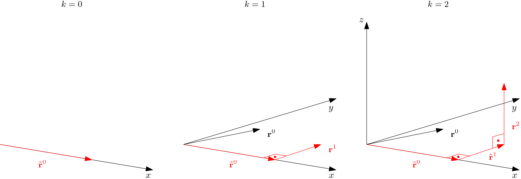
Here, I show the first three iterations of the Bi-Conjugate Gradient algorithm (with the first iteration being the initial guess of the residual vector ). We can see that in the first iteration , we have a simple line for our residual vector of the shadow system. We can't visualise the residual of the original system yet. Think of it as being a line in a different 1D system.
As we go to the next iteration , we can see that is orthogonal to . Both vectors form a plane in the 2D coordinate system. We can also see , i.e. the starting residual vector of the original system, and we see that it is not necessarily orthogonal to .
At the next iteration , we can see that is orthogonal to both and . So, in this case, if we look at the bi-orthogonality equation where we had:
We can say that in the last iteration of , we had and . So, is orthogonal to all previous shadow residuals . We also notice that with each iteration we take, we keep expanding the dimensionality of our system, and for that reason, I stopped at , because I don't feel like attempting to draw in 4D space. You'll have to trust me, though, that it exists; we just can't visualise it.
Similar to the bi-orthogonality, we also enforce these conditions for our search directions as:
Let's pause for a moment and take in what we have done, because if we understand this step, then the rest is just redoing the Conjugate Gradient algorithm derivation, which should be straightforward at this point. I like to look at analogies to help me understand things, so perhaps this one will help you grasp the concept of what the Bi-Conjugate Gradient method is doing.
Think of noise-cancelling earphones. We have a signal we want to hear (in our analogy, we have a system that we want to solve), but this signal contains noise from our surrounding environment. The chatter of people in a cafe, the comforting hum of an aircraft engine 10km above the Pacific, or your annoying neighbour who decides that every day is rock-o'clock.
In the absence of noise-cancelling headphones, by the way, the correct solution to your annoying neighbour is primarily driven by speaker wattage, with your speakers directly attached to your ceiling so that your neighbour can fully enjoy the beat of Helene Fischer. Not my preferred beat, but that was sort of the point. Let's just say I feel sorry for all of the other neighbours, but I regret nothing!
Shortly after that, back and forth, my neighbour had to report a broken water pipe, and water was dripping into my flat (I wonder why ... If you live in the UK, it even rains inside your flat). I'm not sure if he had to pay for it, but let's just say he moved out shortly after that. I digress ...
So, if the music that we want to hear with our headphones represents , then the noise that we hear on top of our music represents the residual . If we can cancel out all the noise, then our residual is zero, and we recover (or ).
If we want to cancel the noise, we need to create ani-noise (i.e. we record the noise in the surroundings and then flip the signal, hoping that this will cancel out all noise from our signal). So we have "music + noise + anti-noise = music" if you want, where "noise = - anti-noise". I know, highly scientific.
In our analogy, if we apply the Conjugate Gradient algorithm now to , knowing that is non-symmetric, we will make an error with each iteration, and that will lead to divergence. This error that we make in each iteration is the noise in our headphone analogy. We want to remove the noise (we want to correct the error of solving ), and so we introduce anti-noise (a shadow residual ), which removes the noise (corrects the error introduced by the non-symmetric matrix).
The anti-noise has to have a specific structure, i.e. we can't just add any noise; it needs to be the exact opposite of the noise around us for noise-cancelling to work. In our analogy, we can't just take any residual, but it needs to be "the opposite" in some way. This opposite is expressed by the transposition of our coefficient matrix, i.e. .
It is related to (the original system) so that if changes, will change as well, and there is a certain connection between the two, just like the noise recorded by the microphone on our noise-cancelling headphones, which is then flipped is related to the noise we hear. If the noise changes, the signal the microphone records will change in the same way. Thus, the noise and anti-noise are connected just like and are.
For any given time interval, our headphones will emit anti-noise ontop of what we are already hearing, and this is like taking one iteration in the Bi-Conjugate Gradient algorithm. This will then successfully cancel the noise, and this is like enforcing orthogonality in the Bi-Conjugate Gradient sense. I have summarised this comparison in the following table as well:
| Headphones concept | Bi-Conjugate Gradient meaning |
|---|---|
| Noise | Error / residual ( ) |
| Anti-noise | Shadow residual ( ) |
| Microphone measuring noise | Action of () |
| Speaker emitting anti-noise | BiCG update step |
| Silence (cancellation) | Orthogonality |
Hopefully, this makes the Bi-Conjugate Gradient method somewhat clearer in what it does. As I said, if we are happy with this, then the rest of the algorithm will feel very natural. It is essentially the same as the Conjugate Gradient method, but we just take combinations from the original and shadow systems to correct the errors introduced by the presence of the non-symmetric matrix.
Let's start by reviewing the algorithm. Since the derivation is essentially the same as in the Conjugate Gradient method (and I must have grown a few more white hairs since I started to write this article 2 months ago), I'll focus on the differences instead of a full derivation. So, just to warn, this is the only section where I won't be deriving everything from scratch, as it has already been done.
We start with our line search update, i.e. finding a new location on our surface that we want to minimise:
We found the residual to be:
So far, so cosmopolitan. Now we make our first subtle change and also introduce the residual for the shadow system:
The definition is exactly the same as the original system, except for the matrix . Remember, this is coming from our matrix , which was the 2-by-2 block matrix with only the matrix and its transpose in it, so that is symmetric.
The next step is to enforce orthogonality. We said that the residuals of the original system all have to be orthogonal to the shadow system's residuals at all previous iterations, though, for the algorithm itself, we only enforce orthogonality between two subsequent residuals or the original and shadow system:
We can insert the definition for and get:
From this, we can find as
Let's focus on the denominator for a moment, i.e. . It is commonly written in a different form, so let's look at that. We know that the search direction can be updated (from the Conjugate Gradient algorithm) as:
Equally, the search direction of the shadow system can be updated as:
In both of these equations, we have the residual given at , but for our denominator that we want to transform, we have the residual given at iteration . We can write the direction update for the previous iteration as:
We just subtracted one from each iteration counter , which resulted in the update to be based on the direction at . Solving this for we get:
Now we can insert that into our denominator and get:
Let's expand the parentheses:
Now we have to remember that we enforce conjugacy. We see that we have in the second term, and two subsequent search directions. Conjugacy requires that two subsequent search directions multiplied by the matrix are zero (this is the key difference between the Conjugate Gradient algorithm and the Steepest Descent method), thus, we can also write:
Therefore, we have:
With this, we can write as:
I have shown this step explicitly here, as it is also usually skipped in the literature. This is a perfect point to pause for a second and mention that when you look up the Conjugate Gradient algorithm in the literature (and its derivatives, like the Bi-Conjugate Gradient algorithm), you will find subtle changes in the algorithms themselves. There are many equivalent ways of how we can write the algorithms, so stick with one source, ideally, and don't mix equations from separate sources. This may lead to an incorrect implementation.
For the search direction update, we already saw the definitions of and . We want to use them now to construct (which will make subsequent search directions conjugate). We start again with orthogonality between the original and shadow system (a constraint coming from all the way back of the Steepest Descent method):
We derived the equation for , and that took a bit more space. If you do the same derivation now with , instead of , you'll arrive at:
And this is the Bi-Conjugate Gradient algorithm! We need to make some choices about the initial vectors, and we have a few constraints. We have one constraint for the initial residual (at ), which is:
That is, residuals of the original and shadow system should not be the same orthogonal. We typically just set them equal at the first iteration. i.e. , which ensures they are co-linear (pointing in the same direction), which means they cannot be orthogonal.
The only other choice we make, similar to the Conjugate Gradient algorithm, is that the first search direction is equivalent to the first residual for both systems, i.e.:
The Bi-Conjugate Gradient algorithm has a tendency to oscillate around the minimum, and thus it usually needs to be stabilised in order to be useful. As a result, we wouldn't use the Bi-Conjugate Gradient algorithm method in practice. However, we do use the stabilised version of this algorithm, so let's have a look at this as well.
Summary of the Bi-Conjugate Gradient method
In summary, the Bi-Conjugate Gradient method can be written down as follows:
- Compute initial residual: .
- Set .
- Loop from to
- Compute search direction length:
- Compute new position on : .
- Compute new residual: and
- Compute correction along :
- Compute new (conjugate) search direction: and
- Compute solution residual: or
- If or , break, otherwise, go back to step 3.
- End
The Bi-Conjugate Gradient Stabilised (BiCGStab) Gradient method
So, I said that the solution of the Bi-Conjugate Gradient method can be oscillatory. Does this sound familiar? When we went from the Steepest Descent method to the Conjugate Gradient algorithm, we said that the search directions in the Steepest Descent method introduced this oscillation, and the Conjugate Gradient algorithm got rid of it by introducing conjugate search directions, not orthogonal search directions.
So, where is the oscillation coming from in the Bi-Conjugate Gradient algorithm? Well, it isn't due to the search directions; these are still conjugate. But, since we use essentially the same (Conjugate Gradient) algorithm to compute the solution, even though our matrix may be non-symmetric, our residual may introduce oscillations. In the Bi-Conjugate Gradient algorithm, the residual was computed as:
We introduced the shadow system for exactly that reason: to get rid of any non-physical results introduced by this equation, i.e.:
As it turns out, this will eventually converge, just like the Steepest Descent method will eventually converge, but it introduces oscillations, which will slow down convergence. In fact, it can even lead to divergence in the worst case. So, we need to stabilise the residual calculation somehow. Let's see how we can achieve that.
There probably is one truth in CFD that we can use whenever we face oscillations: iteratively improve whatever is causing the oscillation. When we later solve the linear system of equations for non-linear equations, well, we iteratively apply until , where is the time index and the iteration counter.
Laplacian smoothing will solve some form of Laplacian equation to smooth a given field for a certain number of iterations . For example, in mesh generation, we may smooth the grid point distributions to get a smoother grid to help us compute a smoother solution. In the residual smoothing technique, we, well, smooth our residuals. This results in greater stability and explicit time stepping techniques, which are otherwise limited to a CFL number of 1, can be run up to a CFL number of 5 or so (personal experience).
In incompressible flows, we introduce smoothing (iterations) to couple the pressure to the velocity field. In fact, this is the main difference between the SIMPLE and the PISO algorithm, where just additional iterations are introduced to stabilise the pressure field.
Later in this article (yes, we are still not done, I'd suggest to put on the kettle and then throw all of your teabags in the kettle, this is not a one tea cup situation, you'll need the entire kettle), we will look at the multigrid approach, and in it, we will introduce smoothing to, you guessed it, stabilise the solution on each grid level.
We use the same idea here; instead of accepting the residual as it is, we are simply going to iterate over the residual, trying to minimise it in some regard. So, let's take the residual, which was given as:
And replace this with an intermediate residual:
We now use this intermediate residual and find a new residual at as:
Notice how Eq.(478) retains the same form of Eq.(476); we have just exchanged here by . So, you may say, that's stupid, we have created an intermediate residual , and the end result is that we have introduced an additional unknown . But no, this isn't stupid; this is exactly what we want!
If we kept in Eq.(478), then all quantities on the right-hand side would be fixed. This means we would have no way of minimising . But, if we replace by a new parameter of which we don't know the value, we can try to find a way to evaluate such that is minimised. This is our goal.
Whenever we want to find the minimum of a function , we know that a possible minimum exists at , i.e. the derivative is zero. It can be either a minimum, a maximum, or a saddle point. In our case, we want to find the minimum of our surface , and we know that it only has a single minimum, with no maximum or saddle points, so we know that will always be a minimum.
Now, looking at Eq.(478) again, we see that the left-hand side is a vector, while the right-hand side only contains an unknown scalar . We cannot minimise every entry in if we only have a single scalar to tune. Thus, we try to minimise some appropriate norm of instead.
Taking the norm of a vector, e.g. the -norm , has the property that a vector is reduced to a scalar value. If we then minimise this scalar value, we know that this will overall minimise the underlying vector, i.e. in this case . Since we want to minimise the norm of , we have to take the norm on both the left-hand side and right-hand side in Eq.(478). This results in:
So, we are left with the task of minimising the right-hand side, i.e.:
In general, for a vector , the -norm is defined as:
Using Eq.(483), we can write this as:
Here, , , , etc. are the products of the entire vector with the first row, second row, third row, etc. of . Now we have the parameter within the square root, so we need to square the expression to be able to solve for . Squaring results in:
This can be written as:
We could also write this as:
This is nothing else than the scalar (dot) product, and so, we can write this with vector quantities as:
We can also write this as a multiplication of a row with a column vector:
This is what we looked at previously, i.e. we saw that we can write when we derived the Conjugate Gradient algorithm. Using this equation, we can multiply terms to get rid of the parentheses:
The rules of transposition state that for two vectors and , the following rule holds:
Let's verify this with the following example:
We have:
We also have:
This shows that the equality does indeed hold for this example (and, in general, for any other real vectors). Using this equality, and setting and , we can see that in Eq.(498), we have these two terms:
We can also write this as:
Using , we can rewrite the second term as:
This can be simplified to:
Substituting and back into our equations, we get:
We can use this to simplify Eq.(498) to:
We differentiate this equation now with respect to :
If we want to minimise this function now, we have to set the derivative (left-hand side) to zero and then solve for . We get:
And this is it. We have found for iteration , so we can evaluate it now so that we are guaranteed to get a new residual which is minimised. This will avoid spurious oscillations once we are close to the minimum. Our job is to now include this new parameter in our derivation, so that we avoid said oscillations.
In the Bi-Conjugate Gradient algorithm, we updated the new location on the surface as:
This corresponded to a residual of:
However, in the Bi-Conjugate Gradient Stabilised version, we changed the definition for the residual by introducing the intermediate residual , which resulted in the additional parameter . So, we need to use this new definition for the residual and then reverse engineer, if you want, the update equation for . Let's do that.
To get started, let's introduce the residual . This is an intermediate residual, and you can think of it as the residual we would obtain from the Bi-Conjugate Gradient algorithm, i.e. with no correction applied to it to minimise . Going from to is what we do in the stabilised version of the Bi-Conjugate Gradient algorithm, i.e. our residual correction.
We can write this intermediate residual as:
Equally, we can find the location before we apply any correction to the residual as:
Inserting into the equation for , we get:
By comparing this with Eq.(477), which was given as:
We see that we have found . Now we return to the definition for the residual of the Bi-Conjugate Gradient Stabilised algorithm, which was given in Eq.(478) as:
This is one equation for , but we also know the general definition for the residual, i.e. . We can set both of these equal and get:
In this equation, we see that we have given on the left-hand side, and we want to isolate that. Once we have done that, we know what our update equation is for the new position on our surface . First, we replace with . This gives us:
We know that we have two expressions for . We compute it using either of the following two expressions:
Let's see what happens when we insert the first expression. We get:
We can subtract and multiply by and get:
Since we want to isolate on the left-hand side, we need to multiply by the inverse of , i.e. and get:
Since a vector multiplied by the identity matrix is the vector itself, we can remove that from the calculation. Don't believe me? Well, I think you and I need to work on your trust issue, but just to show that I am not using black magic here, take the following example:
Happy? Then let's remove the identity matrix from our equation. We get:
We can now insert and get:
We have both and in this equation, so we can cancel it. This results in:
We have found an updated equation, and, if we compare it against the update equation for from the Bi-Conjugate Gradient algorithm, we have:
We see that the stabilised version introduces the additional term . Without it, we get oscillatory residuals; with it, we smooth those residuals. I said that we have two equations for that we could have used, i.e. (this is what we used) and .
If we insert the second definition, that is, , we will obtain exactly the same result.
Ok, so we have a new position on the surface , next we need to figure out what our search direction is. Let's remind ourselves what was, as shown in the following figure, which we saw previously:
is the correction we apply so that subsequent search directions are conjugate to each other (or A-orthogonal). In the Bi-Conjugate Gradient algorithm, we obtained the following relation for :
This definition is dependent on the residuals, and we already saw how we minimise the residual by introducing our new free parameter . Thus, it stands to reason that we need to somehow incorporate the definition of in this equation.
Let's try to come up with an intuitive understanding of how we incorporate in our equation for . Let's look at the following graphical representation:
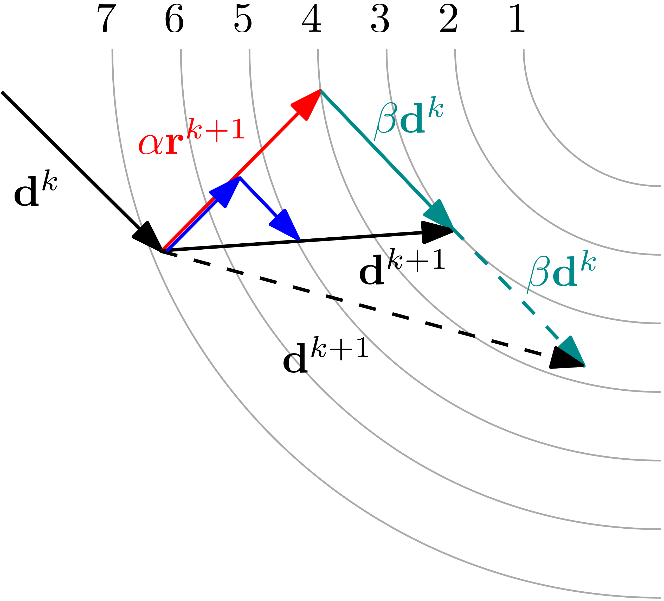
I have shown some contour lines in grey of a surface with some arbitrary values given. We can see that as we move to the top right corner, we minimise the value on the surface .
I have shown the construction for two search directions and . The basic idea is that we first form the residual that is orthogonal to the previous search direction (shown in red), which is scaled by . We use this to move closer and closer to the minimum of . We then also find the conjugate direction to , which will be our new search direction . As we have discussed before, this requires a correction of to our orthogonal residual.
I have shown two possible solutions, one with solid lines and one with dashed lines. We see that the correction of with solid lines gets us to a true minimum (intersecting the contour line where ). If, however, was larger, we would overshoot this minimum and move past it.
So, if you were an algorithm developer, how would you solve this issue? We already know , we have computed , and we want to correct . We see that for a given value of , we want to move a certain amount along . Now imagine was very small, so that we would only move a small distance along . In that case, we would also only need a small correction .
Now, we are going to make the following assumption: For small values of (small move along ), our residuals will oscillate less strongly (require a smaller correction, i.e. is small) when compared to larger values of . We could also say that the ratio of should remain constant, i.e. as increases, we get stronger oscillations and so require more correction.
This parameter isn't arbitrary. is our move along and so we want to scale our correction by this direction. If we look at the figure above, I have shown in red. However, for smaller values of , we need smaller corrections along , i.e. smaller values of . This is shown by the two blue solid arrows.
Therefore, should always be scaled based on . However, looking at the definition for from the Bi-Conjugate Gradient algorithm, which we derived in full, we got:
So, if we simply multiply by , we are just making larger (or smaller). If we divide this now by , which we can think of as a correction factor that minimises our residual, then we ensure that the fraction remains constant, regardless of the stepsize , and so is not dependent on alone. We can then say that the fraction measures the strength of correction.
Therefore, our correction factor becomes:
Comparing that to the version of the Bi-Conjugate Gradient algorithm, we see that indeed we only have the additional scaling term that is added to the definition. You may still not be happy with this explanation, so let's look at some edge cases.
For a symmetric matrix, the Bi-Conjugate Gradient algorithm (and its stabilised form) reduces to the classical Conjugate Gradient algorithm. In that case, we have and so the additional term is and removed from the equation. For , we have no update at all, and this algorithm is stable, but also doesn't update the solution, so it is non really a useful definition.
If we get non-symmetric matrices that also have other unfavourable properties, such as a high condition number, for example, that may be due to poor grid quality metrics, then we have a case of , which then results in . This, too, isn't really helpful, and implementations would typically clamp values for so that we avoid division of (near) zero values.
The final piece of information is the new search direction. For the Bi-Conjugate gradient algorithm, we said that this can be computed as:
However, since the search direction is directly linked to the residual, it too has to change. We do this by analogy. We saw that the residual at can be computed as:
Here, was the intermediate residual. We can also write this as:
Here, is the identity matrix, and any vector multiplied by the identity matrix is the vector itself, i.e. . Since the residual and search direction are linked, we say that if we update the residual in this way, we also want to update the search direction in the same way, i.e. we want to introduce the correction . This gives us:
Multiplying back into the brackets, we get:
With this, we have all the equations necessary to write our Bi-Conjugate Gradient Stabilised. Remember, the key difference between the stabilised and non-stabilised versions of the Bi-Conjugate Gradient method is the introduction of a new, intermediate residual , which also introduces a new parameter that we set so as to minimise the residual in each iteration.
All other equations were simply adjusted to account for the fact that we have a new residual definition, which manifested itself by the inclusion of the parameter in our equations. Thus, we can summarise the method as follows.
Summary of the Bi-Conjugate Gradient Stabilised method
In summary, the Bi-Conjugate Gradient Stabilised method can be written down as follows:
- Compute initial residual: .
- Choose shadow residual: .
- Set .
- Loop from to
- Compute search direction length:
- Compute intermediate residual:
- Compute stabilisation parameter:
- Compute new position on :
- Compute new residual:
- Compute correction along :
- Compute new (conjugate) search direction:
- Compute solution residual: or
- If or , break, otherwise, go back to step 4.
- End
The multigrid approach
We saw how the Conjugate Gradient problem, and its related Krylov subspace methods, turn the problem of finding the solution into a different problem (finding the minimum on a surface ). This worked extremely well, but we also saw quite a bit of math involved to get there.
Oftentimes, though, the simplest solutions tend to be the best solution in real life, and the multigrid approach is very much an example of that. Forget Krylov and its subspace, the multigrid does not get any more complicated than solving a Jacobi or Gauss-Seidel problem (here we go again, yes, Gauss is back).
You can look at the multigrid approach from a math perspective, but I am always more interested in conveying an intuitive understanding of a given problem, so let's do that first, before diving into yet another approach to solve on paper.
Let's say we want to solve a very simple equation, namely the steady-state heat-diffusion equation in 1D, which we have already seen. This is the equation:
Since there is no time derivative, we have to solve this equation implicitly. If we didn't and solved this equation explicitly, this would be our discretised equation:
All temperatures at time level are already known from the initial solution, and there is no temperature at time level , i.e. the next time level, and so we have no way to updating this equation. Instead, we solve it implicitly, and then we get:
Now we do have values at the next time level , and we can solve that again by factorising the temperatures and writing our linear system of equations in the form of . We have:
Let's make one simplification and say that . This allows us to simplify the above equation to:
If we now use 5 cells, for example, then we could write this out in vector-matrix form as:
Now we will simplify that further by just setting the entire right-hand side vector to zero, and we get:
Finally, we need to talk about boundary conditions. I want to impose a temperature of 0 on either side of the domain, which can be achieved by modifying the first and last row of the matrix as:
I have also changed the first and last right-hand side vector entry form to and , which are the values on the boundary, i.e. . Why does this work? Well, let's write out the equation for the first row. We have:
We can simplify that to:
Or, removing the multiplication, we get:
Thus, the first computed temperature will be implicitly set to the boundary condition value . This approach works for Dirichlet problems, as we have it here, but Neumann boundary conditions are somewhat different, and you can read up on implementing boundary conditions for linear system of equation solvers in my article on boundary condition treatments.
We can repeat the same for the last row and see that due to exactly the same reasons.
What would be the expected solution? If I have a metal rod and I heat it on both sides with the same temperature, it stands to reason that we would expect the temperature to be uniform within the rod, i.e. the same temperature should be present everywhere in the rod after a sufficient amount of time has passed.
So, if we set the temperature to 0 (degrees Celcius or Fahrenheit, let's not debate what 0 Kelvin would look like) on either side, we would expect the temperature to be zero everywhere in the rod. In essence, this is a very boring problem to solve, but one where we know what to expect, and so we can now focus on what happens to the solution as we solve .
So, in order to solve this system, we need to supply an initial condition, and I am proposing to solve it with the following 4 different initial conditions/solutions:
- Condition 1:
- Condition 2:
- Condition 3:
- Condition 4:
I am just using some kind of sine function with different wave lengths, and I have plotted the initial conditions in the figure below, as well as the final solution (which is just a flat line and there to sense check that the computation was done correctly and found the right solution). I am using here a spacing of and a total of 40 cells.
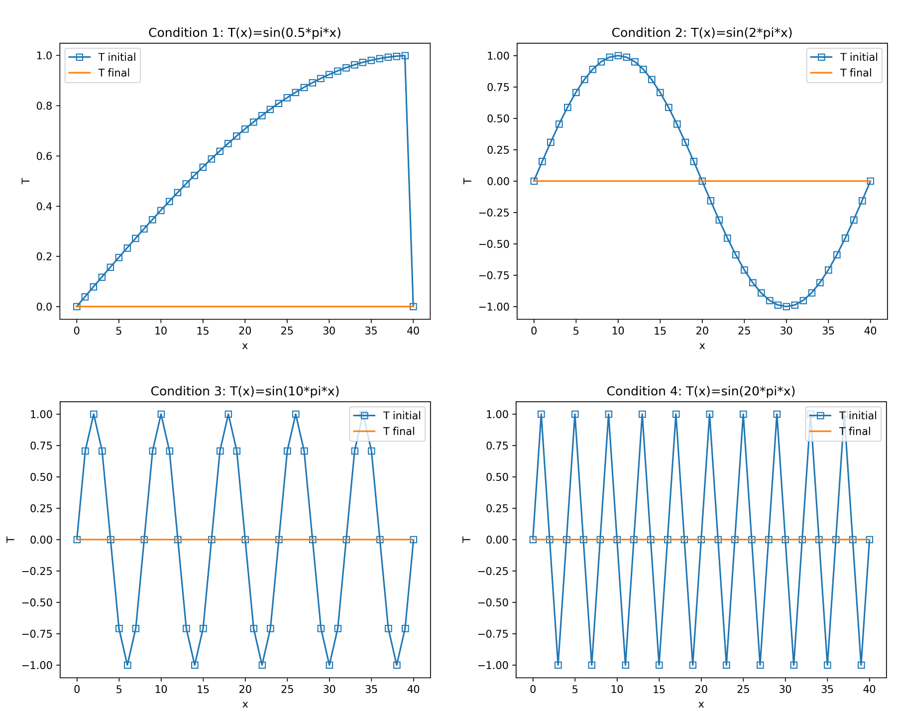
I am using hollow square markers as well, so you can see where values are stored. We see that the wavelength reduces as we go from condition 1 to 4; that's all. Before you read on, I want you to make a guess or prediction.
In a second, I will solve this problem for you using the Jacobi iteration, and all I want you to tell me (you have to shout really loudly at your screen for me to hear you), which of these initial conditions do you think will converge the fastest and the slowest, and why?
Well, let's look at the solution. I am solving this system with the code that I will present in the next section in more detail (specifically, code listing 1). So, if you wonder how we can solve our problem with the Jacobi method, you have the code there.
The table below shows how many iterations it took to solve this problem with the Jacobi solver.
| Initial condition | Jacobi iterations | average temperature |
|---|---|---|
| Condition 1: | 3331 | |
| Condition 2: | 938 | |
| Condition 3: | 43 | |
| Condition 4: | 1 |
Hmmm, this is odd, isn't it? I have spent quite a bit of time telling you that the Jacobi method (and Gauss-Seidel, for that matter) are slow, and we shouldn't be using them. But now, all of a sudden, we see that yes, while some initial conditions are taking their sweet time to converge, there are (special?!) cases in which the convergence down to machine precision () happens in a single iteration. How is this possible? Is Jacobi the underdog that takes the fight to the Conjugate Gradient algorithm after all?
Not quite, and the solution may require some explanation. So, the table above shows the number of iterations required to converge the solution to . We see that as the wavelength is reduced (going from condition 1 to 4), the number of iteration required to do that drop monotonically. We also see the average temperature, which is zero analytically, and should be close to zero numerically (which it is in all cases).
So, why does condition 4 only take a single iteration to converge? For that, let me solve this problem with you, on paper (or, well, on screen). I will simplify the problem a bit by adding a time derivative, so we are solving now:
The reason this is simpler is that the time derivative will now introduce temperatures at time levels and , allowing us to solve this explicitly. However, the end result will be exactly the same; as we approach a steady-state solution, which is described by your original equation , the solution will be the same as Eq.(538), as, by definition, the time derivative becomes zero as the solution turns steady-state.
So, if we discretise this equation now with an explicit time stepping procedure, we have:
We now set and, for stability, we choose a small time step of say so that our explicit time integration will not diverge. Then, we solve this equation for and obtain:
We see that for condition 4, we have values oscillating between -1 and 1, and if we picked 3 consecutive values for , say, at (assuming we start counting from 0, i.e. is the second entry in the temperature array), then we can read off the following values from the figure above (from the initial condition):
Let's insert that into our equation above:
Since we have and , the residual becomes , and this is why we are getting convergence in one iteration; we have found the correct solution (down to machine precision). Let's do that as well for some points on the first condition, i.e. with the longest wavelength. The folowing values are taken for :
If we insert these into our equation, we get:
Thus, we had a value of , and the updated value at is . Only the third digit after the comma has changed its value, and the difference is of the order of . This is tiny, considering that we have to get this value down to 0, which is the solution we know is correct.
For that reason, initial condition 1 took the longest to converge, because it needed to make many tiny corrections to the temperature profile before achieving an average temperature of zero in the domain (e.g. our metal rod). This is also illustrated by the following two animations, where we can see that the longer wavelength requires a lot more iterations to get the temperature profile down to zero compared to the shorter wavelength initial condition:
So, what can we learn from this? There are two key takeaways here:
- Large wavelengths (relative to our grid spacing) take a lot of iterations to converge
- Small wavelengths (relative to our grid spacing) take a few iterations to converge
The key here is relative to our grid spacing. Let me explain. Below, I have sketched out the same temperature solution on two different grids. The grid size can be seen by the ticks on the x-axis, and we see that we have a lot more ticks (grid nodes) on the left than on the right. Therefore, we can say the mesh on the left is a fine grid, while the mesh on the right is a coarse grid.
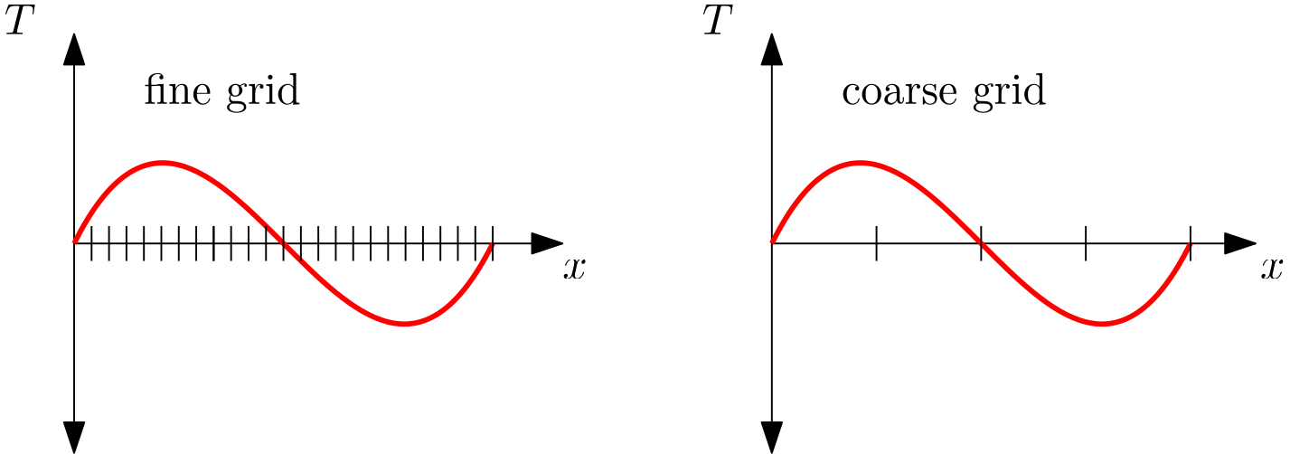
Now, the solution is the same; on both grids, the temperature has a similar sinusoidal behaviour, the only difference is the grid spacing. Based on what we have discussed thus far, if we want the temperature to reduce to zero, i.e. if that is what the final solution dictates, then which of these two cases will find this solution faster? The case on the right, because the oscillations of the temperature profile appear as high frequency oscillations compared to its grid size.
Now, you may be saying, that is all good and fine, but, in reality, the temperature, or any other fluid dynamic quantity we are solving for, like the velocity or pressure, does not have a sinusoidal behaviour, and you would be correct, most of the time, anyway. I'm sure some academics will throw the Taylor-Green vortex problem, or some other artificially created test case, in my face to tell me that we can have a sinusoidal behaviour.
Be that as it may, let us start with again, and see where this sinusoidal behaviour is coming in. We know that is exact, i.e. if we have found an analytic solution for , then it will satisfy the right-hand side exactly. But we are doing CFD, and CFD isn't an exact science.
Just because we are throwing integrals and partial diffentials around like candy on the Colgne Carnival doesn't make it any more correct. Complexity itself isn't evidence of correctness. In fact, if we look at remarkable achievements in Physics, we may quote Newton's , or Einstein's , because they convey complexity through a simple equation. No one in their right mind would bring up .
Let's face it, if medical doctors are body mechanics, then CFD practitioners are fortune tellers. I digress ...
We have accepted that, at best, we are computing an approximation to . If is the exact, analytic solution, then we can say that at each iteration we perform using a Conjugate Gradient algorithm, for example, we approximate the system and we obtain a solution .
Let's introduce the residual again. We said that the following relationship holds for an exact equation:
However, if we now consider instead, the right-hand side is no longer zero, and we express that with the residual , i.e.:
Let's subtract Eq.(543) from Eq.(544), and we get:
We can define the difference between the exact solution and the solution we have at any given iteration as the error from the current computed solution to the exact one, i.e. . If we substitute that back into our equation, we obtain:
As long as the error is non-zero, we will have a non-zero residual. This should make sense, even if it just is from a mathematical point of view, i.e. if we multiply the coefficient matrix by a zero vector, it will return a zero matrix-vector product.
But Eq.(546) tells us something more. We can replace our original equation by an equivalent system of the form . In this system, we no longer solve for the quantity of interest (e.g. the temperature, velocity, pressure, etc.), but instead for the error to the exact solution.
How does the error behave? Well, when I have talked about the von Neumann stability analysis (and thus error modes in our solution), we decomposed the error into, well, drum roll please ... sinusoidal waves!
This is the first building block we need to understand multigrid methods. The second one is a relatively straightforward concept to explain, with what we have already seen. Since we have now introduced the error as the source of the sinusoidal behaviour, and not the quantity of interest , let's go with that in the following description, i.e. we will look at the sinusoidal error behaviour, rather than some arbitrary temperature with a sinusoidal behaviour.
In the following picture, what I have done is to plot the error on an initial fine grid (which I have labelled grid level 0). Then, for each grid below this, I am taking away every second grid point, successively coarsening the grid until we only have 4 grid points left on grid level 3, compared to the 32 grid points on grid level 0.
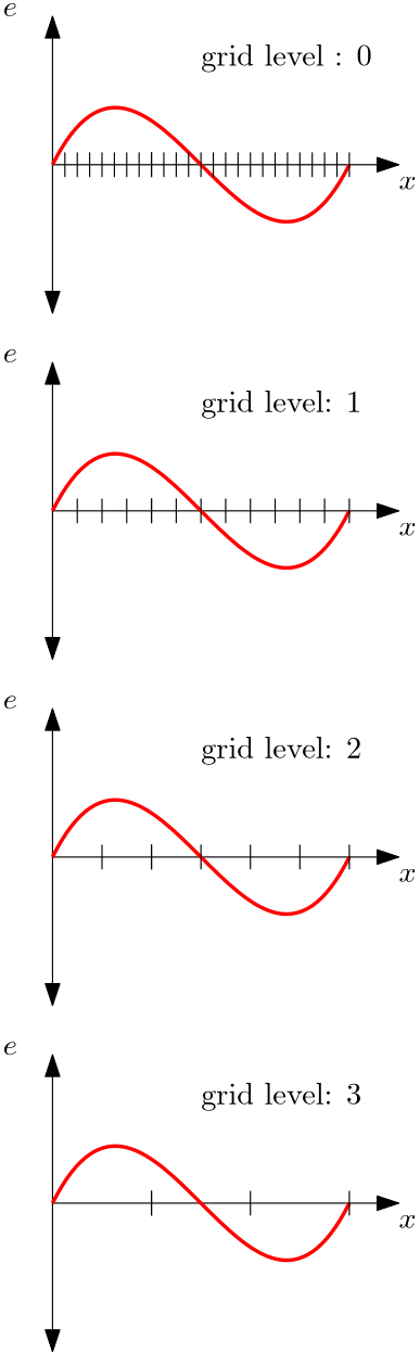
The error is staying exactly the same in its shape; nothing is changing about it (and thus, the underlying quantity, like the temperature, velocity, pressure, etc., that it represents). The only thing that changes is the grid on which we solve it. As a result, the error appears like a low frequency error relative to grid level 0, but has transformed to a high-frequency error on grid level 3.
The multigrid approach, as the name suggests, constructs a series of grid levels on which we solve the solution, going from fine to coarse and back to the fine level for each iteration/timestep. The idea is that by doing this, all error modes will eventually appear like high-frequency errors on the coarsest grid and thus disappear on that grid level.
By doing so, we have seen that high-frequency errors will quickly be damped by any numerical solver. There is no need to go complex here and so it is rather common to use a simple Jacobi or Gauss-Seidel algorithm here. As best as I can tell, the three big CFD solvers Fluent, StarCCM+ and openFOAM all use Gauss-Seidel for their multigrid, so despite this primitive algorithm, it is rather commonly used (we just can't get rid of Gauss, no matter how hard we try!)
Since our linear solvers are now essentially dampening the error , instead of solving , we call our linear solvers smoothers in the context of multigrids. That is, we use the Jacobi or Gauss-Seidel method to dampen the error. Remember, once the error becomes zero, the residual must be zero as well according to . And, once the residual is zero, we recover .
To put all of that into perspective, we started by solving directly, using the Gaussian elimination or LU decomposition. That was effectively forming the inverse of and we were solving . We then looked at approximations, like the Jacobi or Gauss-Seidel algorithm, which iteratively satisfied without forming the inverse .
We then pivoted to an entirely different problem by looking for a minimum on a surface which was equivalent to solving , i.e. when we discussed the Steepest Descent and the Conjugate Gradient algorithm. When we talk about the multigrid, we also dodge the more difficult question of solving and focus on smoothing the error so as to drive the residual down to zero.
There are now three things we need to consider. First, how do we get from the fine grid to the coarse grid and back again? Second: How many grid levels should we consider? Third: In which order should we go from the fine to the coarse grid and back?
Let's address the first question using the following figure:
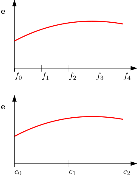
In this simple example, as well as the one provided in Figure 35, we can go from a fine grid level to a coarse grid level by simply throwing every second grid point away.
Going from the fine grid to the coarse grid means we simply copy the values from the fine grid into the coarse grid. Using Figure 36, we have:
Where the points and indicate points on the coarse and fine grid, respectively. If we want to go in the other direction, i.e. from the coarse grid to the fine grid, we use a weighted interpolation.
For example, if we are on the coarse grid and we want to find the value of a quantity on the next finer level, say at , then we can compute that value as:
If we are dealing with more complex grids, for example, unstructured grids, then we simply have to change the weights in our interpolation. In this case, both and are equally far away from , and so they both contribute an equal (or 50%) to the overall interpolation.
If we go from a fine grid level to a coarse grid level, we say this is a restriction step. If we go from a coarse grid level to a fine grid level, we say this is a prolongation step, although you may see some non-standard terminology in the literature every now and then.
The second question we wish to answer is how many grid levels we want to construct. Typically, we construct as many grid levels as it makes sense. You probably don't want to end up with a single cell on the coarsest grid level, but a few hundred cells, roughly, is where I have seen most multigrids to operate at on the coarsest grid level. Your application may require different values, but see this as a rough guesstimate.
The third question is how we traverse from fine to coarse and back to fine. These are referred to as cycles in the multigrid literature. There are a few different cycles that have been proposed, though the most frequently used ones are the V-cycle, the W-cycle, and the F-cycle.
The following figure demonstrates how the V-cycle is implemented:
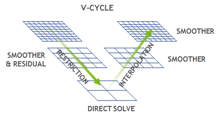
We start on the finest grid and then smooth the error on it, before going to the next coarser grid level, only to repeat the smoothing step. We do that until we reach the coarsest grid level, where we do actually now solve the linear system exactly (or, at least to within a specified residual threshold). Since we only have a few hundred cells, at best, on the coarsest level, this solution becomes cheap. After we have done that, we prolong the solution back to the finest grid, where we smooth the solution on each grid level.
When I say we smooth the solution, we only really run a few iterations. Remember, we want to smooth the error, not solve , so solving for only a few iterations is justified. Typically, we may run around 3-30 iterations on each grid level, depending on how much smoothing we want to apply.
The V-cycle is perhaps the most widely used, but other cycles are available. The following figure provides an overview of perhaps the most frequently used cycles:
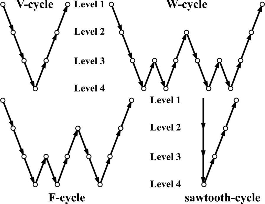
Since these look like some of the letters of the alphabet, we have decided to name them after letters in the alphabet, but, as is tradition in science, we have restricted ourselves to using a Western alphabet (and, of course, in some cases, the Greek alphabet).
In any case, we can see 4 different grid levels, where level 1 represents the finest grid and level 4 the coarsest grid. Going from a finer to a coarser grid is a restriction step (going down in the figure above), and going from a coarser to a finer grid (up in the figure above) is a prolongation step.
So, if we wanted to summarise multigrids, we could do that as follows: First, we acknowledge that errors (sinusoidal modes) reduce quickest on coarse grids. As a result, multigrids aim to solve the same problem on different grid levels to transfer low-frequency errors on fine grids to high-frequency errors on the coarsest grid. We apply a smoother to dampen error modes on all but the coarsest grid level. On the coarsest grid level, containing a few hundred cells, we solve the problem exactly.
If this all made sense up until now, then you have understood most of the multigrid approach. It doesn't get much more complicated than that, but there are two terminologies used that we need to be comfortable with
- Geometric multigrids (GMG)
- Algebraic multigrids (AMG)
Geometric multigrids, or GMG, are what we have looked at thus far. That is, we construct coarser levels of our initial fine grid to construct a hierarchy of grid levels, until the coarsest grid level only contains a few hundred cells or so. Now, on paper, this works very well, and I have chosen my examples thus far very carefully, either coarsening a 1D mesh or restricting our discussion to 2D, structured grids, as seen in Figure 37.
However, let's assume we have a fully unstructured grid, with mixed elements. Take the following 2D example:

This mesh features polygons, triangles, and quad elements. Not sure why you would want to construct a mesh like this (and the question is entirely pointless because I created it), let's say that is the mesh you have been given by your grumpy German supervisor. If you wanted to perform coarsening of this mesh, how would you go about it?
One approach is through agglomeration. Instead of taking cells (nodes) away, we simply merge neighbouring cells into coarser cells, as shown in the following example:
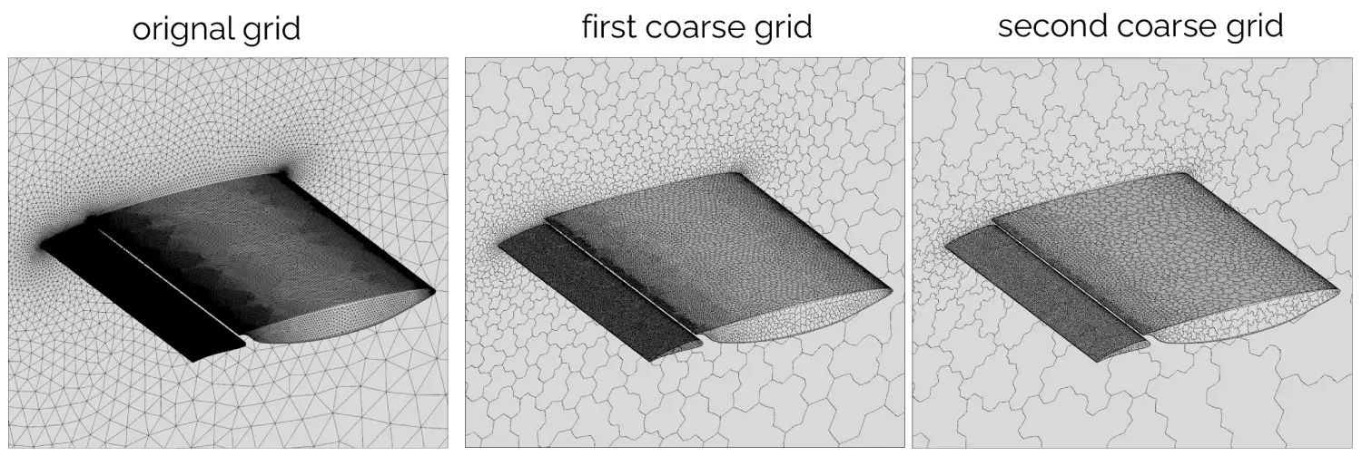
It is still somewhat of a geometric approach, but at least we do not need to provide the grid levels ourselves. Instead, they can be automatically generated by considering the fine (original) grid only.
If you are a CFD developer and you want to implement a multigrid, but you don't want to mess with the mesh itself, what can you do? Well, let's say we have 1 million elements on our fine (original) grid. We may then construct a few mesh hierarchies, let's say, with 100,000 cells, 10,000 cells, 1,000 cells, and finally, 100 cells, so 5 levels in total.
If we look at the effective system we are solving on each grid level, i.e. (we should say smoothing, rather than solving), then we can say that on the finest grid we have a 1 million by 1 million matrix and two one million column vectors and . On the next grid level, we have a 100,000 by 100,000 coefficient matrix and two 100,000 entries column vectors and . This continues down to a 100 by 100 coefficient matrix and 100 element column vectors.
So, in essence, we only construct our different grid levels so that we can construct a new linear system on each grid level. Once we have done that, we don't care much for the grid hierarchy itself anymore. So, if we can, somehow, coarsen our original 1 million by 1 million coefficient matrix and its corresponding 1 million elements column vectors, then we do not have to construct actual grids.
I would call this a multigrid-in-spirit-but-somehow-cheating approach, as we are essentially doing what the geometric multigrid is doing without the need for creating multiple grids (which I have to assume is where the name multigrid comes from).
But, I have come to the realisation once again that I am just born too late and I wasn't around when people came up with a name that stuck in the CFD literature, and so, instead of saying multigrid-in-spirit-but-somehow-cheating, we use the boring of algebraic multigrids. I suppose this name is alright as well ...
So, let's discuss how algebraic multigrids work in some detail, to get an idea of what they are doing.
Algebraic multigrid approaches
Our goal is to take a system of and reduce it in size. A naive approach would be to simply throw away every second line, and this would work for the simplest of problems (like a 1D mesh), but for arbitrary 3D unstructured cases, we need to investigate the matrix a bit more. I'll present a simple problem below, which is taken from a 1D approach, but while it is simple in nature, the same discussion holds for more complex cases as well.
First, let's start with a simple Poisson equation that we have already looked at in great detail. Let's use a model matrix that describes a typical Poisson problem, and we focus on the matrix alone here. For a 5 by 5 matrix (i.e. 5 points in a 1D mesh), we have:
This is essentially the matrix that solves the problem we saw before in Figure 36, i.e.:
If we pick row 3, the diagonal coefficient tells us the value at the location on the fine grid or on the coarse grid. But, we can also see that we have two neighbours, i.e. and (as we have entries in columns 2 and 4 on the third row). Compare that to cell 1 or 5 (in row 1 and 5), which only have connections to one other cell, as these are on the boundary.
We say that cell 3 at has a stronger connection to its neighbouring cells than cell and , and thus, we give the cell at more importance. Once we have finished this computation (assigning importance to cells), we pick the one with the highest priority. If there is more than one with the same level of priority (i.e. the same number of connections), we pick one at random from this subset.
We designate this cell as a coarse cell, which received the label here. On the fine grid, this cell corresponds to , which in turn is connected to and . We now ensure that each fine grid node/cell has coarse-grid cell neighbours. That is, and need to be connected to coarse-grid cells. By ensuring that and coincide with coarse grid cells, we satisfy this requirement.
In any case, we always want boundary cells to be coarse grid cells as well, so that these do not change. We need to impose the boundary conditions here, and if we allowed these cells to be coarse-grained away, we would have no reliable way of imposing boundary conditions.
Now, we have to build the prolongation operator. This is a matrix , where the number of rows is equal to the number of cells on the fine grid, and the number of columns is equal to the number of cells on the coarse grid. In our case, becomes a 5 by 3 matrix.
Our goal is to construct a matrix that can take a vector containing all elements on the coarse grid (i.e. 3 elements in our example) and produce a vector that represents all variables on the fine grid (i.e. a vector containing 5 elements).
Since in our example cell , , and are already part of both the fine and coarse grid, we can start to construct the prolongation matrix as:
If we now take a column vector and multiply it from the right with , we get:
We can see that the first, third, and fifth elements just retain the values of , , and . This makes sense, as these cells were identified to be on both the fine and coarse grid, so we would expect to have the same values here on both grids. But what about cells 2 and 4, i.e. at location and ?
Well, remember back how we handled prolongation (interpolation) before on the geometric multigrid. If we only have information at and , and we want to interpolate the value to node , we can achieve this through:
This is just the weighted interpolation we saw before. For unstructured grids, the factors of 0.5 may change. Equally, we can compute the value at to be:
With that knowledge, we can update our prolongation matrix to:
Let's multiply by a coarse grid column vector again, and we get:
So, the prolongation matrix is just a convenient shorthand notation to do the interpolation (prolongation) for us in one go, without us having to loop over each cell.
Once we have the prolongation matrix defined, we can now start to reduce our original matrix through the following operation:
Here, the subscripts and refer to the coefficient matrix on the coarse and fine grid level, respectively. Since we have both and available, let's carry out the construction of . First, we compute the right multiplication:
Then we compute:
The resulting matrix is now a 3 by 3 matrix, which has reduced from our original 5 by 5 matrix. So, without taking any geometric information into account (apart from the weights in the interpolation, which can be computed from the original grid, though), we have found a smaller coefficient matrix to solve in our problem.
We are almost done. Let's look at our original system on the fine grid, i.e.:
We said that the fine grid solution could be obtained from the prolongation matrix and the solution on the coarse grid, i.e.:
We can insert that into the previous equation and get:
If we now multiply the entire equation by , we get:
We just showed that is the coefficient matrix on the coarse grid, i.e. , so we have:
What about the term on the right-hand side? In our example, we have a 3 by 5 prolongation matrix multiplied by a 5 element column vector. From matrix vector multiplication, we know that the resulting vector of this product must be a 3-element column vector; thus, we can say that:
This is now the right-hand side vector for the coarse grid. We can write this as:
This is just the original system , but now solved (smoothed) on the coarser grid. And that is the multigrid for you. A simple yet elegant solution to solve partial differential equations.
Or is it? What? A curveball? Drama?
Well, you see, multigrids are somewhat of a divisive topic, and people have strong arguments for and against them on either side. In this regard, I am Switzerland and keep my opinion to myself, but let me give you the run down of the problem.
To really understand the issue, we need to understand the mathematical character of a partial differential equation. We can have elliptic, parabolic, and hyperbolic equations, and, as luck would have it, there is an entire article on that topic alone for you to get lost in.
In a nutshell, elliptic flows are those where there is no restriction on the propagation of information. The pressure changes on one end of the domain, and that change in pressure is instantly felt on the other side of the domain, regardless for how far away it is.
The classic example of where that can be seen in nature is the flow around an airfoil, where the streamlines start to turn away from the airfoil before they reach the airfoil itself. No one is telling them that there is an obstacle in front of it, yet they voluntarily start to go around the airfoil without knowing that there is one.
Then, we have parabolic and hyperbolic flows, where we have so-called characteristics in our flow.
A good example of a characteristic is a shock wave, for example. If we have the same airfoil travelling at supersonic speeds, we get a shock wave and all of a sudden, the streamlines do not turn away from the airfoil before they reach it, but rather, they start to deflect only upon reaching the shock wave. The only difference here is the compressibility, i.e. for incompressible flows with have an elliptic behaviour, and for compressible flows (Mach 1 and greater), we have hyperbolic flows.
If I told you that elliptic and hyperbolic flows are different, this may be a confusing statement, but most would intuitively understand that there is a difference between incompressible and compressible flows, and that is a good enough approximation for our current discussion.
In the article on the mathematical characteristics of partial differential equations, I show that we can turn any elliptic equation into a parabolic or hyperbolic equation by adding a time derivative. This alone alterns the eigenvalues of our system, producing real eigenvalues which in turn produce a parabolic or hyperbolic behaviour.
Now, let's think about what that means. If I have an elliptic problem, we typically talk about the pressure Poisson equation, for example, i.e.:
Here, is some right-hand side term, either a constant or a vector. If I introduce a time derivative now, we have:
Only by introducing this time derivative, I change the equation from elliptic to parabolic. Now, let's say we want to find a steady state solution. Then, both Eq.(565) and Eq.(566) will give us the exact same solution. But the way we get to the solution will be wildly different.
In Eq.(565), we have no restriction in the propagation of information, i.e. as I have stated before, elliptic equations allow information to travel instantaneously. Therefore, we can construct as many grid levels as we want, smooth the error modes, and restrict and prolong as much as we want. The convergence rate is going to be a function of the number of grid levels alone.
However, what about Eq.(566)? Now we have a time derivative, meaning that we impose, for each time step, a limit on how much information can travel (which is proportional to the time step size ). This limits the usefulness of our multigrid approach, and the multigrid efficiency is now a function of the number of grid levels and the time step.
For that reason, multigrids, while extremely powerful for elliptic equations, are not able to unleash their full potential in CFD. However, even the little bit of potential they do show is enough for all major CFD solvers to make use of them. They are just that powerful.
A quote I once heard from a defender of multigrids said:
If you don't use multigrids, you are just too stupid to understand them
A source I'd rather not reveal
Well, I am slightly paraphrasing here, but you get the point. Multigrids are difficult to use in CFD as they don't really lend themselves to the problem we solve. A common approach is to use multigrids only for pure elliptical equations, such as the pressure Poisson solver in incompressible flows (SIMPLE, PISO, PIMPLE, Pressure Projection, etc.), but, with some fine-tuning and parametric studies, you can get efficiency also out of multigrids for the entire Navier-Stokes equations.
Like many other CFD people with too much time on their hands (clearly a time before I had kids), I engaged in parametric studies on comparing multigrids with Krylov subspace methods to unearth the holy grail of performance. Like many before me, I failed. In the end, I have found there to be little difference, and, you may be able to squeeze a bit more performance out of multigrids if you are willing to invest in them (i.e. implementing clever algorithms).
When I was at the German Aerospace Center (DLR), that is what one of my colleagues did. The multigrid was a heated topic when I left. It seems I left at the right time.
In any case, multigrids have downsides as well, and I did cover some of them in my article on parallelisation. In essence, if you solve a problem with 1 billion cells, using 100,000 processors, you probably don't want to create a multigrid down to only a few hundred cells; you are going to have fewer cells than processors.
In these types of scenarios, you may be better off with a Krylov subspace solver, like the Conjugate Gradient algorithm. But, of course, be my guest and perform your own parametric studies. But if you do, make sure you have a strong brew next to you. Yorkshire gold is likely the only (legally available) substance on the market that will see you through the parametric study. Don't fall for espresso; you need more tea in your life!
Preconditioning
Thus far, we have looked at solving linear systems of equations, and in the process, we have covered classical methods like the Gaussian elimination and its derivatives (or impostors?!). We also looked at matrix-free algorithms like the Jacobi and Gauss-Seidel method, as well as Krylov subspace methods (predominantly the class of Conjugate Gradients) and the multigrid approach.
We have come across a lot of different tools that we can use to solve , and we have always had one big concern in mind: efficiency and speed.
There is no use in solving our linear system if it takes ages to do so. We saw that the Gaussian elimination procedure scales with , and so it really isn't ideal for large systems of equations. On the other hand, the Conjugate Gradient algorithm was really efficient and allowed solutions within a few iterations, at least for a simple toy problem.
We have now exhausted all possible routes; of course, we can devise even better Krylov subspace methods that subsequently map out a path on that brings us closer to its minimum with each step we take, but there really isn't any point in doing so. Any improvements will be marginal.
Instead, if we really want to make leaps in speeding up our computations, we need to address a fundamental issue of iterative linear system of equations, which we loosely talked about at the beginning of this article.
We talked about the condition number, which I introduced in Eq.(62), and which was given as:
I want to construct a simple model equation and then play around with it and see how it affects the condition number. Let us discretise the unsteady heat diffusion equation in 1D, given as:
In discretised form, this becomes:
We can write this now in terms of coefficients in front of our temperature values:
Rearrange this equation so that all terms at time level are on the right-hand side, and all terms at time level are on the left-hand side, we get:
Combining elements on the left-hand side gives us:
We can write this in the compact form , with given as:
In Addition, we have the vectors and given as:
Let's create this matrix in a simple python code and then observe how the condition number changes as we make changes to the paramter that make up the matrix. The parameters we are free to change here are , , and . These are set based on our meshing, time step size, and difussion strength, respectively, i.e. we have full control over these parameter.
1 2 3 4 5 6 7 8 9 10 11 12 13 14 15 16 | import numpy as np def get_condition_number(N, dt, alpha, dx): A = np.zeros((N, N)) D = np.ones(N) * (1/dt + (2*alpha/dx**2)) L = np.ones(N - 1) * (-alpha/dx**2) U = np.ones(N - 1) * (-alpha/dx**2) A = np.diag(D, k=0) A += np.diag(U, k=1) A += np.diag(L, k=-1) condition_number = int(round(np.linalg.cond(A))) return condition_number |
This code constructs our coefficient matrix by first assembling the main diagonal D (line 6), as well as the off-diagonal in the lower (L, line 7) and upper (U, line 8) matrix. These are then assigned to the matrix A (created on line 4) on lines 10-12. I am using numpy here, which has a function to compute the condition number of a given matrix.
Now, we can construct a matrix by calling the following function from Python, using some default parameters:
1 2 3 4 5 6 | N = 100 alpha = 1.0 dt = 1.0 dx = 1.0 condition_number = get_condition_number(N, dt, alpha, dx) print(condition_number) # will print 5 for these parameters |
So, let's use this function and create a few different matrices and then observe how the condition number changes as a response to our input parameters. First, let's look at what happens when we increase the timestep :
| dt | alpha | dx | Condition number |
|---|---|---|---|
| 0.1 | 1.0 | 1.00 | 1 |
| 1.0 | 1.0 | 1.00 | 5 |
| 10.0 | 1.0 | 1.00 | 41 |
An increase in means we are running our simulations with a larger CFL number. If we are simulating a case without any periodic transient motion, a high CFL number means we can get our simulation to converge faster. However, we also see that an increase in also increases the condition number. So, we may be tempted to increase the CFL number for fast convergence, but the convergence behaviour will be influenced by an increased condition number.
Next, let's see what happens when we change the strength of the diffusion, i.e. :
| dt | alpha | dx | Condition number |
|---|---|---|---|
| 1.0 | 0.1 | 1.00 | 1 |
| 1.0 | 1.0 | 1.00 | 5 |
| 1.0 | 10.0 | 1.00 | 41 |
Again, an increase in (increase in the strength of diffusion) leads to an increase in the condition number. To a certain extent, this makes sense. An increase in means we are simulating the flow with larger time gaps, and so the flow will change faster between two time steps than for a simulation with a smaller .
An increase in has the same effect, in that it induces strong flow between two timesteps and so larger changes between to timesteps are expected as increases.
Next, let's see what happens when we are changing the mesh spacing :
| dt | alpha | dx | Condition number |
|---|---|---|---|
| 1.0 | 1.0 | 0.01 | 3746 |
| 1.0 | 1.0 | 0.10 | 366 |
| 1.0 | 1.0 | 1.00 | 5 |
Here, we see the opposite effect: a decrease in increases the condition number, while both an increase in and were required to increase the condition number. We can also see that a decrease in mesh spacing affects the condition number differently, obtaining significantly larger values for it, due to its quadratic presence in the equation.
Unfortunately, the condition number seems to be increasing whenever we are trying to positively affect our simulation. For example, decreasing the mesh size is generally desired to resolve a simulation more accurately. At the same time, to accelerate convergence, we may be tempted to increase the timestep. Both of these actions increase the condition number.
In the case of decreasing the mesh size, not only do we have to spend more time now to solve our simulation for each timestep (iteration), as we have increased the total number of cells, we also have to run our linear system of equations solver for longer because our condition number has increased.
To demonstrate that as well, let's s create a very simple model example, even simpler than the matrix we have just constructed. The matrix we will introduce is:
Here is a scalar value that we can change, just so that we change the structure of a bit, and thus influence the condition number. Increasing has the same influence as increasing or decreasing , for example, in our previous example. I don't want to obfuscate things here, but rather look at what happens when we start to change the structure of the matrix. But, this change is not arbitrary, as I said, it can be traced back to changes like or .
The right-hand side vector is just set to ones everywhere, and we don't even care about the solution . We only care about it in the sense that we want to compute the residual . We will use that to judge when a solution has converged. So, we need to construct this coefficient matrix and vectors, and then solve it with a suitable method.
Let's use the Jacobi method, which we introduced in Eq.(139), which was given as:
We need the inverse of the diagonal (which will be ), the right hand side vector (which will be just a one for all entries), the (strictly) lower and upper matrices, which are given as , i.e. we just subtract the diagonal from the coefficient matrix . represents the initial solution or solution from the previous iteration.
We can implement that into Python as follows (using numpy again):
1 2 3 4 5 6 7 8 9 10 11 12 13 14 15 16 17 18 19 20 21 22 23 24 25 26 27 28 29 30 | import numpy as np def jacobi(A, b, eps=1e-6, max_iter=100000): N = len(b) x = np.zeros(N) D = np.diag(A) LU = A - np.diagflat(D) residuals = [] residual_norm = 1 converged = False for k in range(max_iter): # jacobi update x_new = (b - LU @ x) / D # compute normalised residual (residual is 1 at the first iteration) res = np.linalg.norm(A @ x_new - b) if k == 0: residual_norm = res residuals.append(res/residual_norm) if res < eps: converged = True return x_new, k + 1, residuals, converged x = x_new return x, max_iter, residuals, converged |
On line 8, we use a special function from numpy, called diagflat, which will essentially create a 2D matrix and we can set the elements on the diagonal directly through a 1D vector (here, D is a 1D vector obtained on the previous line using the diag function, which extracts a 1D vector (diagonal) from a 2D matrix).
On line 16, Eq.(139) is implemented, and then on lines 19-23, I do compute the residual and scale it so that the first residual (at k=0) is always 1. Normalised residuals allow us to ensure that we always converge to the same level of accuracy, i.e. in this case, to a convergence tolerance of , so computations with different matrices are comparable.
We can then go ahead and call the function for different matrices, which in turn have different condition numbers. This is implemented here in the main() function:
1 2 3 4 5 6 7 8 9 10 11 12 13 14 15 16 17 18 19 20 21 22 23 24 25 26 27 28 29 30 31 32 33 34 35 36 37 38 39 40 41 | import numpy as np from matplotlib import pyplot as plt def main(): # input parameters N = 100 scales = [1.0, 1.001, 1.01, 1.1, 2.0] for scale in scales: # construct a coefficient matrix with 2 on the main diagonal and -1 on the off-diagonals with offset 1 diag = 2.0 * scale * np.ones(N) off_diag = -1.0 * np.ones(N - 1) A = np.diag(diag) A += np.diag(off_diag, k=1) A += np.diag(off_diag, k=-1) # right-hand side vector b = np.ones(N) # Condition numbers condition_number = np.linalg.cond(A) print(f"Condition number (exact): {condition_number:.2e}") # Solve using the Jacobi method _, it_jacobi, residual, converged = jacobi(A, b) print(f"Jacobi iterations: {it_jacobi}, residual: {residual[-1]:.3e}, converged: {converged}, ratio: {(it_jacobi / condition_number):.1f}") plt.loglog(residual, label=f'Cond: {int(round(condition_number, 0))}') plt.xlabel("Iteration") plt.ylabel("Residual") plt.title("Influence of the condition number on convergence") plt.legend() plt.savefig("convergence.png", dpi=300) if __name__ == "__main__": main() |
On line 7, I define the parameter , which we use to change the magnitude of the main diagonal of . You can see that I am defining a list here, so I want to check how convergence is affected by a number of different scalar multipliers. On line 22, I am computing the condition number again based on the matrix we have assembled on lines 11-16. On line 27, we call the Jacobi method that we looked at in the previous code section.
If the rest of the code doesn't make that much sense, or you just actively hate Python (why?!), don't worry; understanding the code isn't really the point here. I just wanted to give you enough information to see what I am doing and run the code alongside me if you wanted to.
After running this code, I am getting the following results:
| Condition number | Iterations | Residual | Ratio |
|---|---|---|---|
| 4134 | 33107 | 1.007e-7 | 8.0 |
| 1348 | 10799 | 1.007e-7 | 8.0 |
| 192 | 1536 | 1.009e-7 | 8.0 |
| 21 | 168 | 1.044e-7 | 8.0 |
| 3 | 24 | 1.139e-7 | 8.0 |
We can see that the convergence of the Jacobi method is significantly affected by the condition number. As I have claimed before (and now demonstrated), an increase in the condition number leads to an increase in computation cost, in this case, in the form of having to perform more iterations before converging to the same level of accuracy.
What is interesting to see here is that if we take the ratio of the number of iterations to the condition number, we get a constant ratio of 8.0. Obviously, this number would change if we changed, for example, the convergence threshold or other parameters. The ratio itself isn't necessarily interesting; the fact that the ratio is constant for all cases is.
What that tells us, again, is that a larger condition number will demand more iterations. In this case, since we have computed the condition number explicitly, we could estimate the number of iterations required based on the condition number. Typically, we don't have the condition number given, but it just shows us that there is some structure in the relation between the number of iterations required and the condition number itself.
One last thing, we can also plot the convergence as a result of the residuals plotted against the iterations. In a log-log plot, this is what we would obtain:
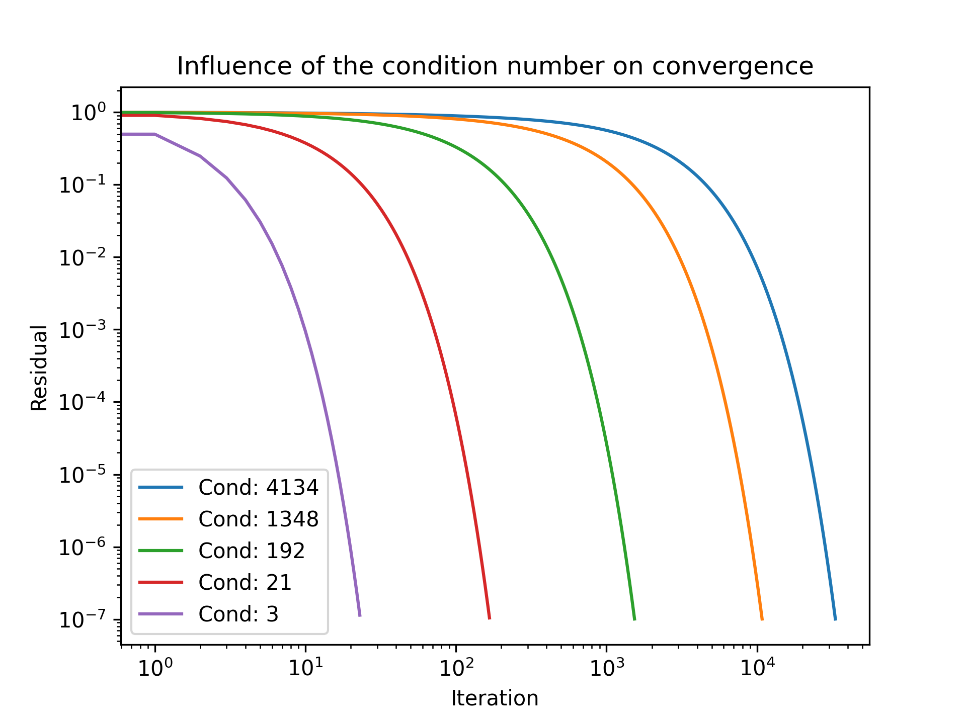
What is interesting in this plot is that the convergence behaviour is, again, identical; the only thing that changes is a stretching of the residual curve towards a higher number of iterations.
So, let's recap: The condition number is a function of the smallest and largest eigenvalues. These, in turn, are dependent on the numerical simulation parameters like the timestep size or the mesh spacing . For typical CFD applications, we get very high condition numbers and so even the best Krylov subspace methods may still require a substantial amount of work before getting close to a solution.
So, now we have to turn to ourselves again and ask, what can we do to circumvent this issue? Let's do some brainstorming. Here is my list of suggestions:
- Modify the simulation so that parameters are optimised to reduce the condition number
- Realise that CFD isn't for us and take up a role as a management consultant
Both options do not appeal to me. For the first option, well, I mean, why are we doing CFD in the first place? To get answers for a specific problem. If we are now trying to please the algorithm to get better results, we should be a YouTuber, not a CFD engineer. And for the second, what even is a management consultant?
Moving on. The sooner we accept that large condition numbers are a thing, the sooner we can accept that we have to deal with them somehow. But let's try to come up with an example that we can exploit for our own advantage.
If you and me ever met up in real life, and someone gave both you and me an apple (and both of us didn't have any apples beforehand), how many apples do you now have? You may say 1, and you would be correct. Now, if you asked me, I could say "I have exactly as many apples as you". That is a very different answer, but equally right. Now, let me write this in a very complex equation:
The money invested in my higher education didn't go to waste ...
So, both you and I have an apple. Now we both eat our apples, how many apples do we have then? If we can stop being nerdy for a second and assume that our body is a system boundary (i.e. technically we still have an apple, dissected into parts, disolving in our stomach), we both have lost an apple, so:
Wicked stuff! One could also write:
So, what I have just demonstrated (arguably a level of detail that isn't necessary) is that we can manipulate an equation by performing the same operation on both sides. The left-hand side and right-hand side values may change (you either have 1 or 0 apples), but the equality is still given (you and I have the same number of apples after receiving and/or eating one, as long as we perform the same action).
So, we looked at an example with a scalar. How about the following equation?:
We can make changes to both sides as well, as long as we do the same action on both sides. For example, we could multiply each side by a matrix and get:
This is perfectly valid, but we should ask ourselves, why do we want to do that? Well, we do have a product of on the left-hand side. Let's assume, for a moment, that , or at least, it is very close to it, i.e. .
If that is the case, we have:
And, to show-off some more of my advanced linear algebra knowledge, we have , i.e. a matrix multiplied by its inverse is just the identity matrix. So, we could simplify this to:
How is this helpful? Well, we have replaced our coefficient matrix with a certain condition number with . A property of an identity matrix is that all of its eigenvalues are 1. So, the smallest and largest eigenvalues are 1, the ratio of is still one, and so the condition number of the identity matrix is .
Thus, if we are able to somehow get close to an approximation of , we potentially could reduce our computational cost significantly. There is one crucial aspect here that often goes unnoticed: When we talked about direct methods to invert so that we can compute the solution directly as , we said these are expensive as we need to find .
Obviously, if we do a bad job getting computed correctly, our accuracy will suffer. But, in the example we have just looked at, i.e. in:
We say that we are happy with an approximation of , and it doesn't even have to be a good one. However, as long as we have some systematic way of constructing a matrix that resembles the inverse of the coefficient matrix , we have the potential to reduce the computational cost significantly.
Just to give you an appetite, in a recent article where we looked at the linear system library Eigen3, we solved a linear system with and without a preconditioner matrix .
The results speak for themselves. Using no preconditioner requires 99 iterations to converge that particular simulation down to machine precision (). However, applying the precondition requires zero iterations! Yes, the preconditioner itself solved the entire system. That is the power of a preconditioner (though it is not a representative example, for real CFD simulations, you would see a reduction of iterations, but it wouldn't drop down to zero).
So, without further ado, let us look at what type of preconditioners are available. I will focus on the 3 most commonly used ones. The other preconditioners you'll find in the wild may be fairly similar to these. There probably are also widely different ones, but as far as I can tell, the ones I am showing in the following sections (and their derivatives) are the ones you would use for a CFD problem.
The Jacobi preconditioner
When it comes to constructing preconditioners, we have to strike a balance between effectiveness and ease of construction. If we spend a lot of time on generating a preconditioner, but it then does not help in speeding up convergence, we may end up using more time with a preconditioner. This is clearly not what we want, and any preconditioner that has this property would be a useless one.
Think about it this way: You are running a marathon, and you are hellbent on winning the race, but someone else just got in front of you, and you are now in second position. There are 10 km left in the race, and you resort to performance-enhancing substances. Well, let's say there are about 30 minutes left before you reach the finish line, you wouldn't dope if you knew it would take up to an hour before any effect could be felt.
It is the same with preconditioners. If it takes longer to construct these preconditioners than solving the actual system, we wouldn't use them, and so, we constantly try to optimise either the time it takes to construct a preconditioner or the time gained using a relatively simple preconditioner.
On a completely irrelevant sidenote, I prefer technology doping, and since my Nike shoes got banned from the Olympics, I use that as an excuse for why I am not winning gold medals for the motherland. It most certainly has nothing to do with the fact that my annual sugar consumption raises the national average, regardless of the country I am currently in, or my unhealthy relationship with Yonsei University's Cream Milk Bread

Am I the only one who finds it a bit odd that a university is mass-producing dairy products and shelling them out to unsuspecting foreigners? Last time I checked, universities were in education and research, but perhaps I have been doing my job wrong the whole time! Who is to tell ...
Let's take stock of my kitchen. I do have a bit of a tea obsession, and currently I am obsessed with finding the best sweetener for my royal milk tea creations (and this isn't even the first time I have mentioned it ...).
Now, some of you may say sugar. Wrong! Sugar is a good everyday fuel, but we are looking for tea taste sensation, not merely average tea enjoyment. Besides sugar, I also have in stock 1.5L of the finest coffee syrup money can buy (or rather, how much my wife allows me to spend on sugar), melted brown sugar, vanilla syrup, and finally, Earl Grey Tea Base, which I can only describe as a tiny bottle of magic. There is a list of syrups I still have to go through on my shopping list.
On that note, if you have any idea what kind of syrup MegaCoffee uses in their Royal Milk Tea, I must know! Send me an email, but also, I find the King must know. Please also send your recipe suggestion to:
His Majesty The King Buckingham Palace London SW1A 1AA
Despite all the sugar and syrups in my life, I remain a healthy BMI of . Well, that is what I believe anyway, it's a Heisenberg uncertainity dilemma, i.e. I can't consume sweet royal milk tea in uncontrolled dosages and know my BMI at the same time ...
So, preconditioning, right? Jacobi, let's give this a spin. In our experiment before, we saw that by changing the elements on the main diagonal of , we could change the condition number. For example, the timestep size only appears on the main diagonal, while the diffusion strength and the grid size also appear on the off-diagonal terms.
The Jacobi preconditioner is now saying that we should just take the diagonal of a matrix , invert it, and then multiply by the matrix again. We could write the preconditioner in this case as:
We now multiply that by our original system . This gives us:
We can explicitly evaluate now , which is:
Let us decompose that further into our upper, lower, and diagonal components, and we have:
Essentially, what the Jacobi preconditioner does is to reduce the magnitude of the diagonal entry to one (and we get the identity matrix here). If we now have a diagonally-dominant matrix (the diagonal entries are much larger than the off-diagonals), then we could expect the condition number to reduce. Should we give it a try?
I'll repurpose the same example from before. The results for changing , , and are shown below, now also showing an additional column for when the preconditioning is applied:
| dt | alpha | dx | Condition number | Jacobi preconditioner |
|---|---|---|---|---|
| 0.1 | 1.0 | 1.00 | 1 | 167 |
| 1.0 | 1.0 | 1.00 | 5 | 167 |
| 10.0 | 1.0 | 1.00 | 41 | 167 |
| 100.0 | 1.0 | 1.00 | 366 | 167 |
| dt | alpha | dx | Condition number | Jacobi preconditioner |
|---|---|---|---|---|
| 1.0 | 0.1 | 1.00 | 1 | 1 |
| 1.0 | 1.0 | 1.00 | 5 | 167 |
| 1.0 | 10.0 | 1.00 | 41 | 312 |
| dt | alpha | dx | Condition number | Jacobi preconditioner |
|---|---|---|---|---|
| 1.0 | 1.0 | 0.01 | 3746 | 64 |
| 1.0 | 1.0 | 0.10 | 366 | 95 |
| 1.0 | 1.0 | 1.00 | 5 | 167 |
This is, perhaps, a bit on the surprising side. When we apply the Jacobi preconditioner, we do not always see an improvement in the condition number! In fact, it seems there are more cases in which the condition number increases than cases in which it decreases. What gives?
Well, we have been running experiments here with random values, and we haven't really explored which of these parameter combinations would actually make sense to use in a simulation. For example, we typically have time step values that are larger than the grid spacing, and so cases which have do not make that much sense. In the case where and , we see that the preconditioning makes the system worse, but the system we are solving in the first place is likely not a good one anyway.
For CFD applications, it is more common to have . For example, in Table 9, we have and . This is much more representative of a CFD problem we would actually solve, and we can see that preconditioning here is effective.
So, the cases we tend to solve in CFD tend to benefit from the Jacobi preconditioner, but we should keep in mind that it can make things worse. If we think about our trade-off between ease of construction and effectiveness, then we see that the Jacobi preconditioner is very much on the extreme side of being easy to construct. It doesn't get much simpler than dividing the coefficient matrix by its own diagonal entries.
In terms of effectiveness, well, we are paying a price here. It can be helpful, but we have also seen that it may make things worse for specific parameter combinations. Thus, the ease of construction is traded for potentially better results, but that is highly dependent on the underlying structure of .
Be that as it may, if you wanted to write your own linear algebra library and support preconditioning, this is likely the preconditioner you want to implement first, as it is so simple and straightforward to implement.
The Incomplete Cholesky (IC) preconditioner
OK, so we have looked at the Jacobi preconditioner, and in many ways, it is a good preconditioner to start with, but there are far better choices out there, and the incomplete Cholesky preconditioner is one of them. It is only applicable to symmetric matrices (e.g. Conjugate Gradient applications), and we will see in the next section how we can handle non-symmetric matrices as well (i.e. matrices used in the Bi-Conjugate Gradient Stabilised).
For that reason, we would use fundamentally different preconditioners for either approach, although we can always use the more general preconditioner (which we will look at in the next section) for symmetric matrices as well.
Cholesky is a bit of an interesting character himself. He worked in the French army and died in combat during the first small disagreement during 1914-1918. He was mapping the world and, just like Gauss, needed to solve matrices as a result. But, since he worked in the military and not in academia, he never thought of publishing his work. He died as a soldier, but we remember him for his contributions as others have taken it upon themselves to publish his work.
He died as a nobody, not knowing that his name would one day crop up in textbooks on mathematics, CFD, and websites on CFD and finding the best syrup + milk tea pairing. I am just sad he never got to try a University-engineered milk cream bread!
The Cholesky decomposition decomposes a symmetric and positive definite cream bread into:
Here, is the lower triangular matrix, but not the strictly lower triangular matrix. The difference is that the lower triangular matrix contains elements on its diagonal, while the strictly lower triangular matrix does not. Thus, for a symmetric 3-by-3 matrix, we can write this decomposition as:
Since we restrict ourselves to symmetric matrices only, we have , and thus we can also write , e.g. . This rewrite produces the following matrix decomposition:
Why is this decomposition useful? Well, if we have a triangular matrix structure of some description, we can usually find the solution of by using the triangular matrix. This is typically achieved in a forward and backward substitution, similar to what we saw in the LU decomposition, where we replace with:
You can see the Cholesky decomposition as a special case of the LU decomposition applied to symmetric matrices, while the LU decomposition works for non-symmetric matrices as well.
Let's carry out the multiplication on the right-hand side to see how we can obtain ! Multiplying , we get:
Now remember, we have the matrix given, and we want to obtain the matrix . We can now set terms in the same rows and columns in matrix and equal. For example, for the first row and column, we get:
In other words, we can find as:
Let's look at the remaining terms in the first row. We have:
Both terms contain , which we already know. Thus, we can solve these two equations for the unknowns as:
Again, since , we have and , so we could also write:
I am sure this little change will make a few people very happy (I am one of them). But also, since we have symmetry here, we only need to solve the matrix for either the upper or lower triangular matrix, since we have .
Let's pick the upper one. The next item we want to solve is , which appears in the second row and second column as:
We know already, so the only unknown here is . We can solve for it and get:
This process continues. Now, it would be too labour intensive to do continue this process manually, so instead, we can generalise the procedure so that we can compute all coefficients in without us having to do any manual subsitutions.
The diagonal terms can be computed as follows:
Let's test that for and , i.e. the diagonal coefficients we have already computed. With , we get:
Since the summation goes from 1 to 0 (i.e. not defined here), the summation goes away. For the case of , we have:
This is what we have obtained before, although I substituted the value for . Good, so now we can obtain all coefficients in for the diagonal. Next, we want to look at off-diagonal components. These are obtained using:
This is valid only for , and we have for . This provides us with the upper triangular matrix, and we can obtain the lower triangular matrix by taking the transpose.
Again, let's test that for a case we have already computed. Let's get compute , which we found to be equal to . Using our off-diagonal formula, we get:
The summation vanishes again as it goes from 1 to 0. With , we get:
This checks out again. And, if you have sufficient trust in me, you can believe me that this works for any of the other coefficients as well. Thus, in summary, we can compute the coefficients of as:
- Diagonal ():
- Off-diagonal ()
With found, we can replace , and have found an effective way to solve . Except, we don't care about this at all.
What we have discussed thus far is, if you want, a simplification of the LU decomposition. That is, we can use the Cholesky decomposition for symmetric matrices to solve for directly if we have a system of the form . But that is not what we want to do. Instead, we want to find a cheap way to construct a preconditioning matrix to reduce the condition number of . In other words, what we want is to find the preconditioning matrix .
This is where we have to introduce the incomplete Cholesky decomposition. The word incomplete suggests that we are not doing a full decomposition, but rather an approximation. This means that we no longer have , but rather, . The crucial step we do now is to set , and we use this preconditioning matrix in our original matrix as:
Since , and , we have that . This brings us close to a condition number of one. How close depends on how incomplete we want our Cholesky decomposition to be. There are typically three options we can choose from:
- IC()
- IC()
- ICT
Here, IC is short for Incomplete Cholesky. The variables in parentheses tell us something about the sparsity of the matrix . In general, our coefficient matrix will be sparse, so if we now apply the full Cholesky decomposition, we may end up with a full matrix . This would increase the computational cost significantly.
In the IC() method, we say that the matrix must have the same sparsity pattern as . That is, if only has two off-diagonals (in addition to its main diagonal), then will also have two off-diagonals and one main diagonal. This is a crude approximation and definitely ensures that is no longer a good approximation for . But it is very quick.
If we use the IC() approach, then we allow for an additional off-diagonals to be constructed by the incomplete Cholesky algorithm. This will improve performance (lower condition number), but it also requires longer to perform the incomplete Cholesky decomposition.
Finally, we can use the ICT approach, which looks at the magnitude of the computed coefficient . If this magnitude is larger than a threshold T, it will be kept, hence the name ICT. If it is smaller, it will be set to 0.
In practice, IC() and IC() are common implementation choices, striking a good balance between accuracy and efficiency.
The Incomplete Lower-Upper (ILU) preconditioner
Conceptually speaking, the incomplete LU (ILU) decomposition is very similar to the IC method. While we said that the IC preconditioner only works for symmetric matrices, since we approximate with (i.e. we only use one triangular matrix, which only works if ). The ILU method works for both symmetric and non-symmetric matrices, and can be regarded as a generalisation of the IC method.
If we wanted to compare both methods, then we could say that IC decomposes as , while in the LU decomposition, we get as . If we look at the approximation of the triangular matrix for the IC preconditioner, we had:
The term arose due to the decomposition of . The lower triangular matrix in the LU decomposition is computed as:
We can see that due to the decomposition of into a matrix and , we also have now entries from in our definition of . The upper triangular matrix , on the other hand, is computed as:
The definition is slightly different, owing to the fact that the diagonal for the matrix is simply set to 1 for each entry, while the matrix retains the true values of the diagonal.
Thus, we can say that in order to generalise the IC method to work with non-symmetric matrices, we change to and therefore we will change multiplications like to . The differences between the definition of and stem from the fact that we have a different diagonal.
In the IC method, we left the diagonal in both and . This then led to the multiplication of diagonal elements by themselves, so that the diagonal components were computed as:
For the matrix, which contains the main diagonal, we had the following definition:
The reason we do not to take the square-root here is because the diagonal elements of are multiplied with the diagonal elements of (which are all equal to 1), not with itself, as we do in the IC method, which then leads to terms like , so that we need to take the square root.
In a nutshell, I hope you can see how the IC and ILU methods are really just one and the same, at least in terms of the idea behind them and how they are constructed; one just uses symmetric matrices, while the other allows a non-symmetric matrix as well.
And, similar to the IC method, we can now construct 3 different variants of our ILU preconditioner. We have:
- ILU()
- ILU()
- ILUT
Just like with the IC preconditioner, ILU() means we keep the same sparsity pattern as . I.e., the ILU preconditioner is only allowed to create entries in if also has a non-zero value in the same row and column. The ILU() method allows for additional -off-diagonals (also referred to as fill-ins, as these off-diagonals do not have any value in the original sparse matrix ), and ILUT only writes entries if the computed matrix components are greater than a certain threshold T.
Preconditioning Krylov subspace methods
OK, so now that we have an idea for how preconditioners work, let us implement them for our Conjugate Gradient algorithm. Typically, we apply preconditioners for Krylov subspace methods, so I will only look at the family of Conjugate Gradient algorithms we have looked at. We saw that preconditioning works by multiplying our system of equations by a system that is multiplied by the preconditioning matrix:
Taking this equation as the starting point, let's subtract the right-hand side. This gives us:
Since we have the preconditioning matrix now in both terms, we can simplify this equation to:
We now write this equation as:
This allows us to define a new (preconditioned) residual which is zero when is zero. Otherwise, if we have , then , too, regardless of the preconditioning matrix . Let's review our Conjugate Gradient algorithm and see where we can incorporate this new residual definition. Once we understand that, applying the same logic to any of the other Conjugate Gradient derivations follows the same steps.
We summarised the algorithm in the following steps:
- Loop from to
- Compute residual:
- Compute search direction length:
- Compute new position on : .
- Compute new residual:
- Compute correction along :
- Compute new (conjugate) search direction:
- Compute residual: or
- If or , break, otherwise, go back to step 2.
- End
In step 2, we compute the residual , so it would make sense to introduce a step here to compute . And this is what we do. But, we do not use it immediately, that is, in what is step 3 above, we do not replace the residual by . Why is that?
When we introduced , we said that we wanted to enforce A-orthogonality (or conjugancy), which is done by the denominator . We say in the Steepest Descent method that we enforce orthogonality between residuals, but in the Conjugate Gradient method, we use conjugacy rather than orthogonality, meaning changes in will affect the path we take in minimising . This wasn't the case in the Steepest Descent method.
Instead, we want to change the definition of , that is, the search direction, which then in turn influences the definition of . In step 7, we compute the search direction as:
Here, we need the residual , which we obtain in step 5 as:
We replace this residual with so that the search direction in step 7 becomes:
In this definition, we also use , which was given in step 6 as:
Now, we used the definition for to enforce our conjugancy. If you look back at how we defined , you may remember that we used the following definition (inner product) during the derivation:
We then replaced the generic variables and by our residual vector , i.e. and , as shown in the numerator and denominator. When we apply preconditioning, we can no longer use this inner product, but instead, have to use a new inner product of the form:
Applying that to our residual, we have:
and
Why is that? Imagine we want to measure the distance on a map (e.g. Google Maps or a similar application). We draw a line on the screen, let's say that line is 4cm long on our screen. This 4cm line corresponds to a distance of, say, 2km on our map, which is displayed on the same screen. Now we zoom into the map, and we see a much more detailed map. If we now draw a second line that is also 4cm in length, it will no longer measure a distance of 2km, but something smaller, as we zoomed into the map.
In this analogy, we can think of the preconditioning matrix as the zooming in operation. As we change the underlying map (zooming in), we can no longer expect that two lines of the exact same length on screen will correspond to the exact same distance measured on the map.
We can also rotate and tilt our map, which are all operations that would affect distance measuring on the map. Let's add one more level of complexity. When we talk about a map, we probably mean some form of 2D projection from what is on Earth to a 2D plane. But the Earth isn't flat (well, let's not get into that argument), and so the curvature of the Earth will affect geometric information on 2D projected maps.
For example, if we draw two lines that have, say, a 45-degree angle to each other on the North Pole and the Equator, they will look completely the same to us standing next to these lines. But, if we project them onto a 2D map of the world, then the fact that the Earth is round-ish will result in these lines looking different on the 2D projected plane.
We can think of preconditioning in this example as the projection of the 3D sphere onto a 2D plane. And, since geometric information is involved again, it will introduce differences.
What is ? It is a geometric statement about two vectors being perpendicular to each other (hinting at a geometric relationship between and ). Thus, if we apply preconditioning to our linear system , we have to change the definition of our geometric measurements, such as . In this case, we simply apply the preconditioning matrix, and so this will be expressed as .
Therefore, our definition for becomes:
Or
In summary, we introduce a new residual , which we use to enforce conjugacy through the definition of , which in turn changes the definition for the new search direction . This search direction provides us with the fastest way towards the minimum of our surface , which changes its shape due to the application of the preconditioning matrix . For that reason, we need to update the definition for so that we still move towards the minimum of .
This is all there is to preconditioning. For the three variants of the Conjugate Gradient family, we can summarise the preconditioned versions as follows:
- Loop from to
- Compute residual:
- Apply preconditioner:
- Compute search direction length:
- Compute new position on :
- Compute new residual:
- Apply preconditioner:
- Compute correction along :
- Compute new (conjugate) search direction:
- Compute residual: or
- If or , break, otherwise, go back to step 2.
- End
Applying preconditioning to linear system of equations
Now that we have derived the equations for the preconditioners, let us see how we can implement that for our Conjugate Gradient algorithm, which gives us the Preconditioned Conjugate Gradient, or PCG, algorithm. I'll implement both the Jacobi and ILU(0) preconditioners for the Conjugate Gradient algorithm to show how both work. We'll also look at the performance of both and see how we really trade efficiency for complexity.
Jacobi preconditioning for the Conjugate Gradient algorithm
The Jacobi preconditioner is the simplest method to implement. The following code modifies our original Conjugate Gradient algorithm we saw before and it introduces the new residual which we have defined as . Remember, the preconditioning matrix contains just the diagonals of the original coefficient matrix , no off-diagonal components, and thus, we are able to easily invert the matrix by simply taking the inverse of the elements on the main diagonal.
Here it is:
1 2 3 4 5 6 7 8 9 10 11 12 13 14 15 16 17 18 19 20 21 22 23 24 25 26 27 28 29 30 31 32 33 34 35 36 37 38 39 40 41 | # preconditioned conjugate gradient using jacobi preconditioner import numpy as np import matplotlib.pyplot as plt A = np.array([[2, 1], [1, 2]]) b = np.array([5, 4]) # simple preconditioner (example: diagonal of A) M = np.diag(np.diag(A)) Minv = np.linalg.inv(M) xnew = np.array([-4, -2]) solutions = [] solutions.append(xnew) r = b - A @ xnew z = Minv @ r dnew = z for k in range(0, 5): xold = xnew dold = dnew rold = r zold = z alpha = (dold.T @ rold) / (dold.T @ A @ dold) xnew = xold + alpha * dold r = rold - alpha * A @ dold z = Minv @ r beta = (r.T @ z) / (rold.T @ zold) dnew = z + beta * dold solutions.append(xnew) # print solution table print('iter | x | y |') print('-----|--------|--------|') for k, x in enumerate(solutions): print(f'{k+1:4d} | {x[0]:6.3f} | {x[1]:6.3f} |') |
The magic happens on lines 9-10 here. First, we define the matrix , containing only the main diagonal of , and then we invert it using numpys inv() (inversion) algorithm. We could have also done this manually as:
1 2 | for i in range(0, A.shape[0]): Minv[i, i] = 1.0 / A[i, i] |
We compute the preconditioned residual on line 17, and then we use that on lines 32 and 33 to compute an updated value for , as well as for the new search direction .
For completeness, I should also mention that the definition for is sometimes changed to include the preconditioned value as well. So, instead of
You may find definitions like:
I haven't done the derivation for it, but inserting this seems to work just as well. I thought I mention it here in case that is what you come across in other literature.
If you run the code shown above, this is what you will obtain:
1 2 3 4 5 6 7 8 | iter | x | y | -----|--------|--------| 1 | -4.000 | -2.000 | 2 | 1.041 | 2.033 | 3 | 2.000 | 1.000 | 4 | 2.000 | 1.000 | 5 | 2.000 | 1.000 | 6 | 2.000 | 1.000 | |
For reference, the standard Conjugate Gradient algorithm without preconditioning gave us:
1 2 3 4 5 6 7 8 | iter | x | y | -----|--------|--------| 1 | -4.000 | -2.000 | 2 | 1.041 | 2.033 | 3 | 2.000 | 1.000 | 4 | 2.000 | 1.000 | 5 | 2.000 | 1.000 | 6 | nan | nan | |
So, no real difference here, apart from the last iteration where our solution had become so accurate that we were getting division by zero errors. What we can extract from this rather simple experiment is that, at least in this case, there is no advantage of using the Jacobi preconditioner. We saw that in our previous experiments as well, where improvements of the Jacobi preconditioners were closely linked to the structure of our coefficient matrix .
In this case, our coefficient matrix is already well conditioned and so preconditioning will likely have a small impact, but at least you have seen how preconditioning enters the picture here.
The Jacobi preconditioner is dead simple to implement, but unfortunately, also as we have seen here, not always effective. So, let us look at the ILU preconditioner, which is slightly more invovled, but usually it provides us with better results compared to Jacobi.
ILU(0) preconditioning for the Conjugate Gradient algorithm
In the Incomplete LU decomposition with zero fill-ins (0), we have to do a couple of things. First, we need to construct the lower and upper triangular matrices and , respectively. Let us remind ourselves how these were defined:
1 2 3 4 5 6 7 8 9 10 11 12 13 14 15 16 17 18 19 20 21 22 23 24 25 26 27 28 29 30 31 32 | import numpy as np def ilu0(A): n = A.shape[0] L = np.eye(n) U = np.zeros_like(A) for i in range(n): for j in range(n): # if A[i, j] is zero, L and U must be zero as well, hence we skip if A[i, j] == 0: continue if i <= j: # compute U[i,j] s = 0.0 for k in range(i): if A[i, k] != 0 and A[k, j] != 0: s += L[i, k] * U[k, j] U[i, j] = A[i, j] - s else: # compute L[i,j] s = 0.0 for k in range(j): if A[i, k] != 0 and A[k, j] != 0: s += L[i, k] * U[k, j] L[i, j] = (A[i, j] - s) / U[j, j] return L, U |
This gives us the two matrices, and with that, we have already done most of the complicated part. Once both the incomplete versions of and have been obtained, we follow the rest of the LU decomposition. As a reminder, the LU decomposition now obtains the solution to through a forward and backward substitution, which is given as:
This is the forward substitution. The backward substitution can be written as:
The forward substitution is implemented in code as:
1 2 3 4 5 6 7 8 9 10 11 | def forward_substitution(L, b): n = len(b) y = np.zeros_like(b) for i in range(n): s = 0.0 for j in range(i): s += L[i, j] * y[j] y[i] = b[i] - s return y |
This works because the forward substitution is solved as:
On the first row, we have , and thus the loop is going from to . So, we skip this loop again and have on the first row. Since has ones everywhere on its diagonal, we do not need to consider it here. To demonstrate that, let's look at the following example:
If I now write out the multiplication for the first row explicitly, we get:
With the knowledge that all diagonal terms are one in the lower triangular matrix, we can set and so end up with:
So, this part checks out, and we have found the first unknown term in the vector . If we go to the second line, according to Eq.(634), we get:
Since we have computed in the previous forward substitution step, only is unknown, and we can solve for it. This repeats until the remaining terms in have been obtained.
The backwards substitution is implemented in code as:
1 2 3 4 5 6 7 8 9 10 11 | def backward_substitution(U, y): n = len(y) z = np.zeros_like(y) for i in reversed(range(n)): s = 0.0 for j in range(i + 1, n): s += U[i, j] * z[j] z[i] = (y[i] - s) / U[i, i] return z |
Let's look at this in code and see why we have this. We are now doing the backward substitution, that is, we are solving . Let's look at the matrix structure first:
If we start looping from the back, that is, we start at the bottom row, and we want to solve for entries in , then we can write matrix-vector multiplication of the last row as:
In this case, the diagonal of contains values that are not necessarily zero, and so we need to divide by it. The row above the last row can then be solved as:
We are doing the forward substitution essentially in reverse, and since has diagonal entries that aren't necessarily one, we also need to divide the result by the diagonal contribution. As an equation, we can write this as:
This equation is what is implemented in the backward_substitution() function above. We can now apply the preconditioner by calling both the forward and backward substitution, provided and are available, and then compute the preconditioned residual . This may require some explaining.
Thus far, we have always said that we want to compute the preconditioned residual as . For methods like the Jacobi preconditioner, we can easily form the inverse of . However, now we are dealing with lower and upper triangular matrices and , which decompose as . Both and will have off-diagonal contributions, making it computationally expensive to invert .
We are back at square one, when we started talking about linear systems. We can't easily invert , so to solve , we can't simply write . Instead, we have to use one of the many methods discussed in this article. The way we get around it in the LU decomposition is to write the original system as this forward/backward substitution step, which solves the linear system of equations without having to compute the inverse of .
Thus, when we are now seeing the inverse in our preconditioned residual , i.e. , this is not the equation we are actually solving. Instead, we multiply by again and have:
This is, well, just , but with different letters. So, we decompose (which really is just in this case) into and , and then we can apply the forward/backward substitution to from the LU decomposition, which gives us the solution for . This is what is implemented in the following function:
1 2 3 4 | def apply_preconditioner(L, U, r): y = forward_substitution(L, r) z = backward_substitution(U, y) return z |
We can now use this ILU decomposition in our Preconditioned Conjugate Gradient algorithm as:
1 2 3 4 5 6 7 8 9 10 11 12 13 14 15 16 17 18 19 20 21 22 23 24 25 26 27 28 29 30 31 32 33 34 35 36 37 38 39 40 | def main(): A = np.array([[2.0, 1.0], [1.0, 2.0]]) b = np.array([5.0, 4.0]) # build ILU(0) L, U = ilu0(A) xnew = np.array([-4.0, -2.0]) solutions = [xnew.copy()] r = b - A @ xnew z = apply_preconditioner(L, U, r) dnew = z.copy() for k in range(5): xold = xnew.copy() rold = r.copy() zold = z.copy() dold = dnew.copy() alpha = (dold @ rold) / (dold @ (A @ dold)) xnew = xold + alpha * dold r = rold - alpha * (A @ dold) z = apply_preconditioner(L, U, r) beta = (r @ z) / (rold @ zold) dnew = z + beta * dold solutions.append(xnew.copy()) # print solution table print('iter | x | y |') print('-----|--------|--------|') for k, x in enumerate(solutions): print(f'{k+1:4d} | {x[0]:6.3f} | {x[1]:6.3f} |') if __name__ == '__main__': main() |
Note that we only construct the matrices and once on line 7, which is then reused throughout the algorithm. We then compute the preconditioned residual before entering the main loop in line 13, which is then updated for each iteration on line 26, after a new residual has been found (i.e. see line 25).
Now, here is what is interesting. If we look now at the results printed by the table at the end, this is what we get:
1 2 3 4 5 6 7 8 | iter | x | y | -----|--------|--------| 1 | -4.000 | -2.000 | 2 | 2.000 | 1.000 | 3 | nan | nan | 4 | nan | nan | 5 | nan | nan | 6 | nan | nan | |
Remember that iteration 1 is just the initial solution, so really, after just a single iteration, we have found the exact solution. In fact, the fact that we are getting not a number (nan) after the second iteration, shows that the solution has found an exact solution after just a single iteration.
Before we jump up and down in excitement, believing we have cracked CFD and found a secret algorithm that solves all of our problems, here are some things to keep in mind:
- Currently, we are only using a 2-by-2 matrix. This is a toy example, and we are not really stress testing the algorithm.
- The matrix itself is already fairly well conditioned. Worse condition numbers, as is usually the case in CFD, will reduce our convergence rate.
Nonetheless, we see that the preconditioner has the power to essentially solve our linear system of equations very quickly, and that is why we need preconditioners for CFD applications.
Well, hopefully you have a better idea about preconditioners now, but I am afraid we have not yet reached the end. Yes, I know, you probably started reading this article yesterday and lost track of time, and now a day has passed, it might be 3am in the morning, and you are so hooked that you can't stop reading. I get it, preconditioners and Krylov subspaces are fascinating, but I'm afraid I can't let you go just yet. Cancel your 9am meeting and put on the kettle, we have one more mountain to climb.
If it makes you feel any better, I remember it snowing when I started writing this article. It is now 25 degrees Celsius (about umpteen degrees in Freedom units), and the winter coat has been replaced by shorts and t-shirts.
Extension of linear system of equations solver to non-linear systems
So, it took me a good 4-5 hours of your time to get to this part of the article. Have you noticed that, thus far, I have always talked about linear systems of equations solvers when we want to find a solution to ? Unfortunately, the Navier-Stokes equations, you know, the ones we try to solve (presumably), are non-linear in nature.
So, whatever I told you in the past few hours isn't relevant; ignore it, we have to start from scratch. Well, not really, it is true that linear system of equation solvers are, well, designed for linear equations, but thankfully, we can extend this to help us with non-linear equations as well.
I should say, though, that what we are about to do is a correction; it is not a new method in its own right. Let me give you an analogy that hopefully makes this clear.
As a teenager, I have learned that if I want to know if Pasta is cooked, or not, I should take one Spaghetto (singular of Spaghetti) and throw it at the wall. If it sticks, it is done; if it doesn't, they will need some more time to cook. As a teenager, I took it at face value, and it worked reasonably well. As a grown-up with an engineering background, I am immediately starting to think whether different surfaces and their roughness will have an influence.
For the love of science, next time when you boil an array of Spaghettos, please take one and throw it at your wall. Feel free to throw it at other objects around the house and note down your results. Feel free to send in your results; that is a joint academic publication waiting to happen!
Now, when I lived in Italy, I made the mistake of sharing this little piece of knowledge with my friends. After they collected themselves and stopped laughing, they asked me how I know if my sauce is done.
You may say this is silly (more silly than throwing spaghettos?), but let's think this through. Let's say I did throw some sauce at the wall to see if it sticks. Eventually, I have to clean up the mess after all of my experimentation has finished. However, I used tomato sauce with a thick red wine base. As a result, my terracotta-painted walls are all stained now. What should I do?
Well, we can paint over the stains. They may still be visible, even if they are mostly covered, but they are still there. Alternatively, I could tear down the wall, reconstruct it, and remove the stain completely.
In this analogy, what we are about to do is paint over the stain. We will extend linear system of equations solvers to non-linear equations by some form of correction, but the fundamental flaw will still be in the system. The results we will obtain are quite good, but we can still see the footprint of using a linear system of equations solver for a non-linear equation.
The idea is as follows. Take the non-linear term in the momentum equation of the Navier-Stokes equation. Any non-linear term will do, but let's just focus on one term:
Here, this term is non-linear because we have twice. In fact, in conservative form, we have:
However, that is only the case for incompressible flows; for compressible flows, the situation is slightly different. If you want to know why, have a look at my write-up on primitive vs. conservative variable formulations. What it does show, though, is that this term is indeed non-linear in .
In any case, let's discretise with a first-order upwind scheme. We have:
Writing this in coefficient form, we have:
So, we can now write our coefficients into our matrix , right? Well, but what about the terms and ? For ever update in the solution, the velocity vector will change, and so the values of will change, too. This means that our matrix will change from iteration to iteration.
Imagine what that means. Imagine we are using the Conjugate Gradient algorithm and then performing an update to get a new velocity field. Since these changes, we also need to change . Even worse, if we now consider the preconditioned version of the Conjugate Gradient algorithm using the ILU preconditioner, we have to reconstruct and for each iteration. This is getting expensive quickly.
What is the solution here? Well, let's write our non-linear term again:
I haven't said anything about what time levels we are evaluating the velocity at. For a fully non-linear treatment, we would have:
But, this introduces the issue that we have just discussed, i.e. the coefficient matrix is constantly changing. Instead, what we can do, is to linearise our non-linear term. What that means is that we replace the velocity in front of the fraction by , which gives us:
Now, the term is still non-linear, or at least sort of. I suppose one could say it is non-linear-ish, or, if German was ever to be brought back as a common scientific language, we would say nichtlinear oder so, so pseudo-nichtlinear, or nichtlinear, wenn man großzügig ist. All highly scientific.
What this means is that when we construct our coefficient matrix , we would be constructing it from the following discretised formula:
Now, all terms that go into the coefficient matrix (i.e. those inside the square brackets) are evaluated at time level and thus do not change during the iterative procedure. No need to change and no need to update our preconditioners. Happy days.
But now we have a different problem. Once we have found a solution to , we have essentially found the solution vector , which in our example would be the x-velocity vector . So, we now have . However, this was computed based on velocity values in the coefficient matrix that came from time level (i.e. our linearisation step). Essentially, we have found a solution to:
However, , and this is important. Why? Because originally we wrote this term as:
Here, both velocity components are the same. Because of our discretisation (and subsequent linearisation), we introduced and . Since these are not the same, we could express that as:
In the CFD literature, this is often acknowledged by writing as . We then have:
or simply:
This is used to show that and are different quantities. So, now that we understand the main problem, and have added some more German vocabular to our ever growing list of "German words I'll never use", we can start looking at our corrections to fix this issue (i.e. painting over the pasta sauce stain on our walls).
The "10-layers of paint" strategy: Picard iteration
The Picard solution is dead simple: We solve the system of equations several times. Once we have obtained a solution for , we update the coefficients in based on the new solution in . We repeat this until , where is the Picard iteration index.
Essentially, what we do is to fix the number of Picard iterations and then solve the system for a specified number of times. We can also check how much the solution changes between Picard iterations. If the changes are getting smaller than a predetermined threshold, we can also exit early from the Picard iteration.
There is some good and some bad news here. The bad news is, each Picard iteration solves one full system from scratch. This is rather expensive. The good news is that we only use it for non-linear equations, i.e. the momentum equations in the Navier-Stokes equations. These turn out to be very quick to solve, compared to the pressure, so even if we solve the same system over and over, it is still cheaper than solving for the pressure.
In our pasta-sauce-stain analogy, the Picard iteration is like taking 10 layers of paint and painting over the stain (solving repeatedly, e.g. 10 times or more). It is somewhat of a brute-force approach, but it works, just like John the Ripper, given enough time.
But, here's the thing. It can be computationally expensive to perform these additional iterations once our system grows large enough. Indeed, most CFD solvers usually skip any form of correction and simply assume . As our CFL number grows, so will the discrepancy between and , and so solutions may behave unexpectedly. This is often overlooked, but it is something holding the accuracy of our solutions back.
But, if we want to include it, then the Picard iteration is a bit like doing a DIY job on the pasta stain. You may save some money, but certainly not time. If you call a professional, you don't have to spend time going to the store, getting paint, painting, cleaning up, etc. A professional comes, sees the problem, knows which paint to use, how many times it needs to be applied, etc. The best part is, it is quick.
The professional in this analogy is what the Newton-Raphson is doing for us, so let's look at that method as well in the next section.
The "Measure twice, paint once" strategy: Newton–Raphson
The Newton-Raphson method employs a bit of additional work upfront before we can solve our linear system of equations, but the effort is worth it. Let's start with a very simple experiment. Let's try to approximate the function . Now, I have given you the exact formula, so we can just compute the solution exactly, but let's say we don't know that and we want to find an approximation of , based only on data that we have available (e.g. some initial data).
If we don't know what is, what can we do? Well, the answer in CFD (and in physics) always seems to be to use a Taylor series. Let's develop the function around some small step size and see what function we get. The Taylor series is given as:
In CFD applications, we would typically use this equation to solve for , which we generally don't know but would like to obtain. In this case, though, we know that , so we can compute as:
If we insert that into our Taylor series, we get:
In other literature, you may find a different derivation. You may find that some would suggest expanding as:
We can carry out the multiplication on the right-hand side and get:
Since we are looking for a small area around where we want to approximate our solution, will be small compared to the rest of the terms, and so we can simplify this expression to:
Knowing that , we can write this as:
That's the same result as we have obtained from the Taylor series. Slightly different approach, but same outcome, i.e, we don't know the solution of (well, we pretend for now that we don't know it, I have given it as ), but given some initial data, if we know how the solution changes if we go by to either side, we can approximate a solution of .
The classic example here is to predict the temperature. Neither you or me can predict the future and state what the temperature is going to be like. But, given some initial data (the temperature right now), I bet you could make a pretty accurate prediction of what the temperature will be like after 1 hour, 1 minute, or even just 1 second. Here, would become , i.e. the time interval after which we want to know the temperature.
So, let's look at a table where we compute exactly using , and then how its approximated value is if we take different step sizes of .
| u | error | |||
|---|---|---|---|---|
| 1 | 1 | 2 | 3 | 50.0% |
| 1 | 0.1 | 1.1 | 1.2 | 9.1% |
| 1 | 0.01 | 1.01 | 1.02 | 1.0% |
| 1 | 0.001 | 1.001 | 1.002 | 0.1% |
Here, we are saying that we fix to be one. Then, we add some value to it and then evaluate using the exact formula and the approximation . I have also computed the error, and we can see that as decreases, we get more and more accurate predictions for our approximation.
This makes intuitive sense: If I asked you to predict the temperature 1742 hours from now, or 1 hour from now, which prediction do you believe will be closer to the correct solution? Here, again, we don't have but rather , i.e. a time interval. The same is true for our function , which we can approximate fairly accurately with our Taylor series approximation.
Why do we bother doing this approximation? Well, let's compare the function we started with and the approximation we obtained:
What can we say about these functions? Well, of course, one is an approximation to the other, but more importantly, the first equation is non-linear (we have , or ), while the second function is linear (or a linearised version of the non-linear function, i.e. we don't have or ).
So how does it help us? Well, let's write out the Navier-Stokes equations, specifically, the momentum equation for an incompressible flow. This is given as:
Let's bring all terms to the left-hand side. This gives us:
Now, this is an equation that we solve for the velocity , so we could say that this is a function of , or . Thus, we could also write this as:
This is still a non-linear equation. However, we want to discretise that now and then solve it with our linear system of equation solver, that is, we need to construct from it. So, if we linearised this equation now around some small distance , we could use our Taylor series that we have developed before as:
In the CFD literature, is usually given as , so, just to be inconsistently consistent, let's do that as well:
So, let's recap what this equation actually tells us, or what we are able to do with it. We have some value of everywhere in our domain. For example, that could be our initial solution, or the solution from the previous timestep/iteration. To compute it, we use the Navier-Stokes equations, which we have written as . So, we have a function with which we can compute everywhere in our domain.
When we want to update it, we want to do so with a linear system of equations solver, so we want to use our Taylor series approximation, as it will linearise a non-linear function. As long as the changes are small enough, we will get a good approximation (our linearised equation will give us an accurate prediction for our non-linear equation).
What we now have to do is to evaluate the derivative , which in the CFD literature is also known as the flux Jacobian, and usually given the abbreviation . Using this short-hand notation, we can write our Taylor series approximation as:
So, the question becomes, how do we evaluate the flux Jacobian ? I have written about that in great detail in the article on Eigen. I have provided a derivation of the flux Jacobian by hand, but also an alternative approach where you compute the flux Jacobian without having to think about it too much, using automatic differentiation. I won't go into detail here again of how is computed, so feel free to read the section in the Eigen article before continuing.
Let us rewrite our linearisation step slightly:
If you have gone through the Eigen article, you will have come across the following flux Jacobian (now for the compressible Euler equations):
Here, we have three lines, because we are considering the 1D compressible Euler equations, where each lines represents one equation, i.e. the first line is the conservation of mass equation (continuity), the second line is the momentum equation, and the last line is the energy equation. From the continuity equation, we get the density , from the momentum equation, we get , and from the energy equation, we get the energy .
Therefore, we could now write our linear system of equations solver as:
In other words, the flux Jacobian is a matrix. So, in this example, what would represent? Well, since we are now dealing with the system of the Navier-Stokes equations, we are solving three equations for three unknown quantities (it is actually 4 unknowns if we consider the pressure as well, which we obtain from the equation of state, though). Thus, must be a vector, which represents incremental changes to the variable we are solving for.
Equally, the right-hand side vector contains the values for the density, velocity, and energy that are obtained from the conservation of mass, momentum, and energy equations. Let us write this as:
Here, I have used the short-hand notations , , and to denote the conservation of mass, momentum, and energy equations, respectively. If we look at this system, then we can say that the flux Jacobian can be evaluated from quantities that we know from the previous time step or the initial guess. The right-hand side is known as well, which is simply the computed values for density, velocity, and energy at the previous time step (or initial guess).
But what about the vector? We don't know this! If I were to say that , , and , then we could also write our linearised Taylor series as:
It all comes back to bloody , doesn't it? Well, but let's think this through. If we solve this linear system of equations now, what do we actually compute? Solving this linear system, we get a solution for , or . But that is not what we are really interested in. is just an increment from some previous value. Thus, once we have obtained this solution, we need to update our solution using the following update equation:
We could also write this explicitly for each variable as:
Here, I am using the superscript and , not and , indicating that this is very much an iterative approach. Just like the Picard linearisation, we need to perform the Newton-Raphson approximation several times before . However, the rate of convergence for the Newton-Raphson is much faster than the Picard iteration, and that is where the additional effort of constructing the flux Jacobian pays off.
Now, if I left it at this point, as many textbooks on CFD do, you would be excused to believe that we actually solve now many smaller linear systems on a per-cell basis, that is, we construct the flux Jacobian for each cell, solve for , and then correct the variables within each cell using these values.
That is not, however, what we do. Instead, we assemble all flux Jacobians into a global, block-structured matrix, which is shown in the following:
Here, each matrix and is a flux Jacobian matrix, containing several rows and columns. We see that there are flux Jacobians on the main diagonal (e.g. ), as well as on the off-diagonals (e.g. ). We get this additional off-diagonal flux Jacobian because when we discretise our equations, we get influences from neighbouring cells. For example, if I want to know the derivative in cell , then I can approximate that as:
So, the discretised equation is coupled to neighbouring cells, and so, additional off-diagonal flux Jacobians appear. If we solved the flux Jacobians on a per cell basis, we woudl be neglecting the influence of all of the off-diagonal couplings, and that would lead to a loss in accuracy.
Summary
How does one summarise an article that has been written for about 3 months, and where I barely remember what I wrote last week? Well, here is my summary; yours may differ.
We started off with a simple example, and I showed how any discretised equation can be written in a system of the form of . We then saw that for an explicit discretisation, the coefficient matrix contains only elements on the main diagonal, and so, we can easily invert it.
Once we introduce an implicit treatment for just one variable, we saw that we introduce off-diagonal components, and this resulted in very costly inversion operations for the matrix , if we wanted to solve for .
We then looked at a few properties of matrices, which we later exploited in various sections, and we all adopted Krylov as one of our new favourite Russian mathematicians, who gave us the Krylov subspace.
We looked at direct methods to solve problems, and we also saw how these are too expensive to be used in practice to solve the linear system of equation exactly.
We then started to look at classical, iterative methods, such as the Jacobi and Gauss-Seidel method, as well as the successive over-relaxed (SOR) version. We tried to improve the convergence rate but ultimately had to accept that this was a lost cause. Instead, we turned to Krylov and saw how a reformulated problem can be expressed, where we now try to minimise some surface , where the minimum of that surface happens to coincide with the solution of .
This allowed us to use geometric search algorithms to find the minimum of , starting with the Steepest Descent method, and then looking at the family of Conjugate Gradient methods, which we subsequently improved through preconditioning, a technique used to reduce the condition number of the coefficient matrix to gain faster convergence.
Finally, we also looked at the multigrid approach and how it can produce impressive results with even simple iterative methods, and that was followed by a discussion on how to extend to non-linear systems, notably the Navier-Stokes equations. We looked at both the Picard iteration and the Newton-Raphson method.
So, what can we learn from all of this? Is it that we cannot do linear algebra without saying the name Gauss at least 42 times? Is it that in France, we leave important breakthroughs in math to soldiers? Or is it that solving is best done by drawing lines on a hypersurface?
For me, it is none of that. Instead, I think the most important takeaway message is that there is a university in South Korea that has specialised in mass producing milk cream breads that is driving obesity rates through the roof (a claim I have no interest in proving scientifically, shoot me).
They just started merging milk breads with Filipine Ube, whatever that is, and I took some time to photoshoot it while I was probably supposed to play with my daughter on the playground. In fairness, she was busy munching through a cheese sausage of unknown nutritional properties (it tasted like fish cake), so I suppose we both were happy.
So, why not make travel plans to visit Korea (I'd recommend the southern part), head to the nearest CU convenience store and get your very own University-grade cream bread?
Acknowledgements
Special thanks to Yagna Chennupati for helping me to improve this article! Check out how you can contribute, too.

Tom-Robin Teschner is a senior lecturer in computational fluid dynamics and course director for the MSc in computational fluid dynamics and the MSc in aerospace computational engineering at Cranfield University.